High-Resolution Estimation of Soil Saturated Hydraulic Conductivity via Upscaling and Karhunen–Loève Expansion within DREAM_(ZS)

Abstract

Quantification of the soil hydraulic conductivity is key to the study of water flow and solute transport in unsaturated soils. Rapid advances in measurement technology have provided a large number of observations at different scales, offering unprecedented opportunities and challenges for the estimation of hydraulic parameters. This paper proposes an inverse estimation method for downscaling of observations on coarse scales to estimate hydraulic parameters on high-resolution scales. Due to the significant spatial heterogeneity, the inversion faces the problems of dynamics-based integration of data at different scales, model uncertainty due to hundreds and thousands of parameters, and computational consumption due to the large number of forward simulations. To overcome these problems, this paper uses an efficient Bayesian optimization ${\mathrm{DREAM}}_{\left(\mathrm{ZS}\right)}$ as an inverse framework, and incorporates an analytical upscaling method and Karhunen–Loève (KL) expansion to infer finer-scale saturated hydraulic conductivity distribution conditioned on coarse-scale measurements. The efficient upscaling method is used to link measurements and hydraulic parameters at different scales, and Karhunen–Loève (KL) expansion is incorporated to greatly reduce the dimension of the parameter to be estimated. To further improve the efficiency of the inversion, a locally one-dimensional (LOD) algorithm is used to solve the multidimensional water flow model at coarse scales. The proposed inverse model is applied in a series of numerical experiments to demonstrate its applicability and effectiveness under different flow boundary conditions, different levels of ratio between coarse- and fine-scale grids, different densities of observation points, and different degrees of statistic heterogeneity of soil mediums.

1. Introduction

Soil hydraulic conductivity is essential information for soil water flow and solute transport simulations to represent hydrological processes such as water storage, release, and transfer in the soil, and is therefore a prerequisite and key link to ensure model effectiveness. Saturated hydraulic conductivity is often spatially heterogeneous and scale-dependent [1,2]. Uncertainty in ground permeability can result in considerable alterations to the response of the porous medium [3,4]. And the simulation process is often time-consuming and labor-intensive to obtain directly in field or laboratory experiments subject to scale constraints [5,6]. In recent years, numerical inversion methods based on field observations have been increasingly used to estimate the hydraulic conductivity of soils [7,8,9,10,11,12,13,14,15,16].

We note that most of the existing studies focus on the inversion of hydraulic parameters in homogeneous or stratified soils using observations at the same scale. However, strong spatial variability often requires us to obtain the spatial distribution of soil hydraulic parameters at a high resolution. Particularly, as the observations are obtained from multiple scales with different means of observation, it is necessary to integrate the dynamic observations at different scales to obtain the hydraulic parameters at the required scales. Thus, the problem boils down to integrating observations at different scales to invert the spatial distribution of soil hydraulic parameters at high resolution. This problem faces two difficulties: first, how to integrate observations on different scales for the inversion of hydraulic parameters on the scale of interest. Here, it is necessary to establish a kinetic relationship between observations on multiple scales and the hydraulic parameters on the scale of interest. The other is how to solve the problem of efficiency and uncertainty of the inversion simulation due to the huge parameter dimensions and the consequent large number of forward simulation calculations.

This study uses Bayesian optimization ${\mathrm{DREAM}}_{\left(\mathrm{ZS}\right)}$ as an inverse framework, and incorporates an efficient upscaling method and Karhunen–Loève (KL) expansion to infer finer-scale saturated hydraulic conductivity distribution conditioned on coarse-scale measurements. First, the ${\mathrm{DREAM}}_{\left(\mathrm{ZS}\right)}$ algorithm is used as a inverse framework to construct the posterior distribution of saturated hydraulic conductivity field in high-dimension soils conditioned on coarse-scale observations. The ${\mathrm{DREAM}}_{\left(\mathrm{ZS}\right)}$ is an improved Markov chain Monte Carlo (MCMC) method proposed by Vrugt et al. [17,18,19,20], which greatly improves the convergence speed of the inverse model compared to the traditional MCMC method. Compared to the basic DREAM (DiffeRential Evolution Adaptive Metropolis) algorithm, it refers to the previous sampling state to adjust the current process in generating each chain candidate, which aims to reduce the number of parallel chains and accelerate the convergence of high-dimensional problems, and has been successfully applied to research in many fields [21,22,23,24,25].

Then, the upscaling method proposed by Li et al. [26] is used to link observations and hydraulic parameters, which may come from different scales. This method is based on the Kirchhoff transformation and the two-convergence theory to propose the macroscopic description of the Richards equation and the effective constitutive relations, rather than equivalent or upscaled flow parameters, as is the case with many parameter averaging approaches such as the stream tube approach [e.g., [27,28,29] and the scaleway approach [e.g., [30,31]. And compared with a number of multiscale numerical methods to calculate the effective constitutive relations, which are formed and solved numerically, the proposed upscaling approaches is based on analytical formulations, which are preferred in practical applications because they are efficient in computation and convenient to use. Simultaneously, within the Bayesian inversion, the using of upscaling method avoids solving the model at fine scales, thus improving the computational efficiency of the forward models. In addition, the local one-dimension (LOD) [32] is used to solve the multidimensional Richards equation to further improve the efficiency of the inversion process.

Within the ${\mathrm{DREAM}}_{\left(\mathrm{ZS}\right)}$ framework, the incorporation of the upscaling method can efficiently integrate the hydraulic parameters and state variables at different scales, but it still has to face the problem of model uncertainty due to the large number of parameters and thus the consequent problems of convergence and efficiency of inversions. This study employs KL expansion to reduce the parameter dimension and thus the uncertainty of the inversion simulation. Karhunen–Loève (KL) expansion is a technique used in data analysis to represent a data set in a more efficient way by decomposing the data into a set of simpler, uncorrelated functions capturing the most significant variations within the data. In Bayesian inference, KL expansion has been an effective approach to represent the random field and is successfully applied in various fields (e.g., [33,34,35,36,37,38]). Through KL expansion, thousands of spatially distributed hydraulic parameters can be reduced to dozens of quantities, which greatly reduces the number of predicted parameters and thus the uncertainty of the inverse simulation.

Therefore, in the framework of Bayesian inference ${\mathrm{DREAM}}_{\left(\mathrm{ZS}\right)}$, combined with the upscaling algorithm and KL expansion, we propose an efficient and effective inversion method to downscale the observations on coarse scales to obtain higher-resolution saturated hydraulic conductivity. The applicability and effectiveness of the proposed method are investigated through a series of numerical examples. Different flow boundary conditions, including constant head boundaries, variable flux boundaries, and mixed boundaries, are considered for two-dimensional soil profiles. We consider soil heterogeneity, characterized by statistical spatial variability include variance, correlation length, degree of anisotropy. We set different levels of mesh coarsening, i.e., inversion of saturated hydraulic conductivity field on fine scales based on different coarse-scale data, to explore the effects of different levels of mesh coarsening on the inverse results. And we investigate the effect of a smaller number of data on the inverse simulation by reducing the number of observation points in the data. Overall, the proposed methodology is validated in a comprehensive manner through a large number of numerical experiments.

The paper is structured as follows. Section 2 describes our numerical inverse model, revisits the upscaling method and KL expansion, and introduces the ${\mathrm{DREAM}}_{\left(\mathrm{ZS}\right)}$ to solve the inverse problem. Section 3 describes the case setup for numerical simulation, including the selection of boundary conditions for water flow, characterization of soil heterogeneity, scaling between coarse and fine scales, and the setup of observation point density. Section 4 provides a thorough assessment of our method’s performance under different model settings. Section 5 summarizes the key findings of this paper.

2. Methodologies

This study is concerned with the reconstruction of the spatial distribution of soil saturated hydraulic conductivity at finer scales based on pressure heads at larger scales. Hydraulic parameters and dynamical data at different scales are integrated within the ${\mathrm{DREAM}}_{\left(\mathrm{ZS}\right)}$ inference framework, incorporating the upscaling method and the KL expansion. The forward model is to solve the macroscopic Richards equation with homogenized soil hydraulic properties using the LOD method. Therefore, this section describes the forward models, including the Richards equation with soil properties, the upscaling method, and KL expansion, and then briefly introduces the ${\mathrm{DREAM}}_{\left(\mathrm{ZS}\right)}$ method.

2.1. Soil Water Flow Modeling

This study considers estimation of saturated hydraulic conductivity in two-dimensional soil profiles. The Richards equation is the most prevalent model to describe soil water flow, as follows in Equation (1):

$$\begin{array}{c}\hfill \left\{\begin{array}{c}C\left(h\right){\displaystyle \frac{\partial h}{\partial t}}={\displaystyle \frac{\partial }{\partial x}}\left(K\left(h\right){\displaystyle \frac{\partial h}{\partial x}}\right)+{\displaystyle \frac{\partial }{\partial z}}\left[K\left(h\right)\left({\displaystyle \frac{\partial h}{\partial z}}+1\right)\right]\hfill \\ C\left(h\right)={\displaystyle \frac{d\theta }{dh}}\hfill \end{array}\right.\end{array}$$

(1)

where h is the pressure head, m; t is the time, $\mathrm{d}$; $C\left(h\right)$ is the change of water content with head, ${\mathrm{m}}^2{\mathrm{m}}^{-3}$; $K\left(h\right)$ is the hydraulic conductivity corresponding to the pressure head, $\mathrm{m}{\mathrm{d}}^{-1}$; and $\theta$ is the water content, ${\mathrm{m}}^3{\mathrm{m}}^{-3}$. The van Genuchten model [39,40] is used to inscribe the soil hydraulic properties, including the water content curve $\theta \left(h\right)$ and the hydraulic conductivity function $K\left(h\right)$:

$$\begin{array}{cc}\hfill \theta \left(h\right)& =\left\{\begin{array}{cc}{\theta }_{\mathrm{r}}+{\displaystyle \frac{{\theta }_{\mathrm{s}}}{{\left(1+{\left|ah\right|}^{\beta }\right)}^{\gamma }}}\hfill & h<0\hfill \\ {\theta }_{\mathrm{s}}\hfill & h⩾0\hfill \end{array}\right.\hfill \end{array}$$

(2)

$$\begin{array}{cc}\hfill S_e& ={\displaystyle \frac{\theta -{\theta }_{\mathrm{r}}}{{\theta }_{\mathrm{s}}-{\theta }_{\mathrm{r}}}}\hfill \end{array}$$

(3)

$$\begin{array}{cc}\hfill K\left(h\right)& =K_{\mathrm{s}}{S}_e^{\frac{1}{2}}{\left[1-{\left(1-S_e^{\frac{1}{\gamma }}\right)}^{\gamma }\right]}^2\hfill \end{array}$$

(4)

where $\alpha$, $\beta$, $\gamma$ are curve empirical coefficients, $\alpha$ is the reciprocal of the inlet value, ${\mathrm{m}}^{-1}$, $\beta$ is the pore size distribution coefficient, $\gamma =1-{\displaystyle \frac{1}{\beta }}\left(\beta >1\right)$, ${\theta }_{\mathrm{s}}$ is the saturated water content, ${\mathrm{m}}^3{\mathrm{m}}^{-3}$, and ${\theta }_{\mathrm{r}}$ is the residual water content, ${\mathrm{m}}^3{\mathrm{m}}^{-3}$.

2.2. Upscaling Method

The upscaling method based on numerical homogenization theory is computationally efficient and convenient to use because of its explicit expression [26]. The macroscopic model of the Richards equation is as follows:

$$\begin{array}{cc}\hfill {\displaystyle \frac{\partial {\theta }^{*}\left(h^{*}\right)}{\partial t}}& =-\nabla ·\left[{\overline{K_{\mathrm{s}}}}^{*}\left(x,{\theta }^{*}\right)\nabla \left(h^{*}+z\right)\right]-0\hfill \end{array}$$

(5)

$$\begin{array}{cc}\hfill {\theta }^{*}\left(h^{*}\right)& =\left\{\begin{array}{cc}{\theta }_{\mathrm{r}}+{\displaystyle \frac{{\theta }_{\mathrm{s}}}{{\left(1+{\alpha }^{*}{\left|h^{*}\right|}^{\beta }\right)}^{\gamma }}}\hfill & h^{*}<0\hfill \\ {\theta }_{\mathrm{s}}\hfill & h^{*}⩾0\hfill \end{array}\right.\hfill \end{array}$$

(6)

$$\begin{array}{cc}\hfill {\alpha }^{*}& ={\displaystyle \frac{1-\gamma }{\gamma \left({\theta }_{\mathrm{s}}-{\theta }_{\mathrm{r}}\right)}}·{\displaystyle \frac{K_{\mathrm{s}}^{*}\left(x\right)}{D_{\mathrm{s}}^{*}\left(x\right)}}\hfill \end{array}$$

(7)

$$\begin{array}{cc}\hfill {\overline{K_{\mathrm{s}}}}^{*}\left(x,{\theta }^{*}\right)& =K_{\mathrm{s}}\left(x\right)K_r\left({\theta }^{*}\right)\hfill \end{array}$$

(8)

where $\theta$*, h*, K*, $D_{\mathrm{s}}$*, $\alpha$* are the equivalent coefficients in the homogenized Richards equation.

2.3. KL Expansion

In order to solve the uncertainty problem caused by a large number of parameter inversions, this study uses KL expansion to reduce the dimension of the parameter space. This powerful technique decomposes a random field into a series of uncorrelated random variables and deterministic coefficients. The key advantage of KL expansion lies in its ability to represent a complex random field with just a few parameters, leading to low estimation errors and broad applicability. Assume that the two-dimensional random field of saturated hydraulic conductivity $K_{\mathrm{s}}\left(x,\omega \right)$ has a mean value of $\overline{K_{\mathrm{s}}}\left(x,\omega \right)$, and that all spatial points on $E{\left[K_{\mathrm{s}}\left(x,\omega \right)-\overline{K_{\mathrm{s}}}\left(x,\omega \right)\right]}^2$ all exist; then, its KL expansion is described as Equation (9):

$$\begin{array}{c}\hfill K_s\left(x,\omega \right)=\overline{K_s}\left(x,\omega \right)+\sum _{i=1}^{\infty }\sqrt{{\lambda }_i}{f}_i\left(x\right){\xi }_i\left(\omega \right)\end{array}$$

(9)

where x is the spatial point coordinates; ${\xi }_i\left(\omega \right)$ is a random field generated using a Gaussian distribution, where $\omega$ is the parameter randomness and in this paper the value is all the same in different samples for control variable; $\left\{f_n\left(x\right)\right\}$ is the eigenfunction series, and $\left\{{\lambda }_n\right\}$ is the series of eigenvalues.

$\left\{f_n\left(x\right)\right\}$ and $\left\{{\lambda }_n\right\}$ are the solution to Fredholm integral equation of the second kind.

$$\begin{array}{c}\hfill {\int }_{\Omega }\rho (x_1,x_2)f_i\left(x_1\right)d{x}_1={\lambda }_i{f}_i\left(x_2\right)\end{array}$$

(10)

where $\Omega$ is the region of integration. The eigenfunction can be decomposed into a linear combination of M orthogonal basis functions.

In the generation of a random field through the use of KL expansion, a set of M (the truncation order of KL expansion) mutually independent random variables, denoted by ${\xi }_i\left(\omega \right)$, is produced. The eigenfunctions and eigenvalue series are obtained through the solution of the integral equations, $\left\{f_n\left(x\right)\right\}$, $\left\{{\lambda }_n\right\}$. Once the integral equation has been solved to yield the eigenfunction and eigenvalue series, the value of the Ks random field is generated by Equation (9), thereby enabling the $K_{\mathrm{s}}$ field to be represented by a small number of M [36].

Figure 1 depicts the magnitude of the eigenvalues for the first 50 orders. It can be seen from the figure that the eigenvalue size decreases rapidly as the order increases, and the eigenvalue sizes of the lower orders are much higher than the higher-order values as a percentage of the eigenvalue size. Therefore, a small truncation order M can be used to approximate the original complete eigenvalue, which can greatly reduce the number of parameters and also ensure the accuracy of the overall KL expansion on behalf of the random field, which greatly reduces the number of parameters required for the inversion. In this paper, the truncation number of the eigenvalues used is M = 30, which contains more than 99% of the total eigenvalues’ size.

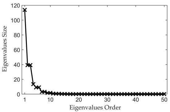
Figure 1. Variation in eigenvalues’ size with order in KL expansion.

2.4. Bayesian Inference with ${\mathrm{DREAM}}_{\left(\mathrm{ZS}\right)}$

In the inversion process, suppose that the model to compute is $f\left(u\right)$, which contains a series of continuously distributed parameters to be solved, u, and a series of observations, $Y_{\mathrm{obs}}$. According to the Bayesian formula, we can obtain Equation (11).

$$\begin{array}{c}\hfill p\left(u\right|Y_{\mathrm{obs}})={\displaystyle \frac{p\left(u\right)p\left(Y_{\mathrm{obs}}\right|u)}{p\left(Y_{\mathrm{obs}}\right)}}\end{array}$$

(11)

where $p\left(u\right|Y_{\mathrm{obs}})$ is the posterior density probability function of u, $p\left(Y_{\mathrm{obs}}\right|u)$ is the likelihood function, and $p\left(Y_{\mathrm{obs}}\right)$ is the probability of the observation arising from the value of the observation, which is a constant independent of u.

In the usual inversion process of MCMC sampling, if the proposed distribution is poorly correlated with the target distribution, a large number of proposed samples are rejected because they fall outside the posterior distribution, which leads to the need for a much higher number of iterations and greatly prolongs the overall inversion computation time. Therefore, an effective parametric inversion algorithm, ${\mathrm{DREAM}}_{\left(\mathrm{ZS}\right)}$, is used in the inversion process of this paper.

${\mathrm{DREAM}}_{\left(\mathrm{ZS}\right)}$ creates the jump vector in $\mathrm{DREAM}$ from the past states of the joint chains [19,20]. Instead of generating candidate samples ${\zeta }^i$ based only on the samples in the current row of the matrix $\mathrm{X}$, all the samples in the current and past state matrices $\mathrm{Z}$ of the chain are used, the equation for obtaining the c candidate sample ${\zeta }^i$ in the i chain is Equation (12).

$$\begin{array}{c}\hfill {\zeta }^i={\chi }_{c-1}^i+(1+e_{\eta })g\left(\psi ,{\eta }^{\prime }\right)\left[\sum _{j=1}^{\psi }{\mathrm{Z}}^{r_1\left(j\right)}-\sum _{k=1}^{\psi }{\mathrm{Z}}^{r_2\left(k\right)}\right]+{ϵ}_{\eta }\end{array}$$

(12)

where: ${\chi }_{c-1}^i$ is the $c-1$ sample on the i Markov chain; $\eta$ is a normally distributed random number with mean 0 and standard deviation $b^{*}$; $e_{\eta }$ is a uniformly distributed random number in the interval $\left[-b,b\right]$; $g(\psi ,{\eta }^{\prime })$ is a scale factor, the value of which is determined by the parameters $\psi$ and ${\eta }^{\prime }$, $\psi$ is the number of parallel chains for generating candidate samples, and ${\eta }^{\prime }$ is the number of parameters being updated in candidate sample ${\zeta }^i$; ${\mathrm{Z}}^{r_1\left(j\right)}$ and ${\mathrm{Z}}^{r_2\left(k\right)}$ are the $r_1\left(j\right)$ and $r_2\left(k\right)$ samples randomly selected from the matrix $\mathrm{Z}$, $r_1\left(j\right)\ne r_2\left(k\right)$, $j,k\in 1,2,\cdots ,\psi$.

In this way, the inversion problem at high latitudes can be solved with a smaller number of parallel Markov chains and shorter chain lengths compared to the traditional MCMC algorithm.

The ${\mathrm{DREAM}}_{\left(\mathrm{ZS}\right)}$ V1.0 software can be downloaded from the https://faculty.sites.uci.edu/jasper/ (accessed on 15 May 2024).

3. Setup for Downscaling Simulations

In this study, numerical experiments are performed with artificially generated dynamic data in two-dimensional heterogeneous soil profiles. Soil water pressure heads are generated based on the spatially distributed hydraulic properties and then treated as observations by adding Gaussian errors as perturbations. The proposed inverse model is demonstrated in a series of numerical experiments where three different boundary conditions of the soil water flow, four levels of scale variances between the fine and the coarse scales, various combinations of soil heterogeneity including four degrees of variances, four degrees of correlation lengths, and four degrees of anisotropy ratios are considered to give a comprehensive applicability and validity of the methodology.

3.1. Parameter Settings for Soil Profiles

The study area is set up as a 5 m × 5 m vertical profile. We choose loamy soil with moderate soil quality, and its hydraulic parameters are from the USDA (United States Department of Agriculture) for different soil texture categories: saturated water content ${\theta }_{\mathrm{s}}$ = 0.4, residual water content ${\theta }_{\mathrm{r}}$ = 0.07, a pore size distribution index n = 1.1, and the reference value of saturated hydraulic conductivity $K_{\mathrm{s}}$ is 0.28 $\mathrm{m}{\mathrm{d}}^{-1}$. Here, the proposed inverse method is performed in heterogeneous soil profiles, with the two most variable parameters ($K_{\mathrm{s}}$ and shape parameter characterizing the pore distribution $\alpha$) exhibiting spatially variable. The “true” two-dimensional $K_{\mathrm{s}}$ fields are generated using KL expansion, with this reference as the mean. $\alpha$ is considered to be the spatially distributed field associated with $K_{\mathrm{s}}$, that is, $\alpha \left(x,z\right)=\sqrt{K_{\mathrm{s}}\left(x,z\right)}$. The spatial heterogeneity is quantified by statistical parameters including the spatial variation variance $\sigma$, the size of characteristic length $\lambda$ (${\lambda }_x$ and ${\lambda }_z$ in the x and z directions, $\mathrm{m}$) and the anisotropic ratios (${\lambda }_z/{\lambda }_x$). These parameters are set as follows: $\sigma$ = 0.5, 1.0, 1.2, 2.0; when investigating the effect of different characteristic lengths on the simulation results, we use an isotropic medium, but with varying characteristic lengths, that is, ${\lambda }_x={\lambda }_z$ = 4, 8, 12, 16 m; when investigating the effect of the degree of anisotropy on the simulation results, we use an anisotropic medium by taking the characteristic length in the x-direction to be 4, but in the z-direction to be 16, 64, and 180, which gives us four degrees of anisotropy, i.e., v = 1, 4, 16, 45.

3.2. Settings for the Fine- and Coarse- Scale Grids

The scales of the observed and needed parameters often do not coincide; here, we opt to downscale from the observed data on the coarse scale to obtain the hydraulic parameters on the fine scale. The fine-scale grid in this paper is set as 128 × 128 in the 5 m × 5 m study domain, on which the saturated hydraulic conductivity field will be estimated, that is, 16,384 parameters will be estimated. In order to explore the effect of upscaling size on the inversion results, the coarse-scale grid on which the observations are obtained is set to 128 × 128 (the same as the fine-scale), 64 × 64, 32 × 32, 16 × 16, and 8 × 8. The saturated hydraulic conductivity will estimated via the inverse model conditioned on observations from one of these coarse scales.

3.3. Settings for the Observations

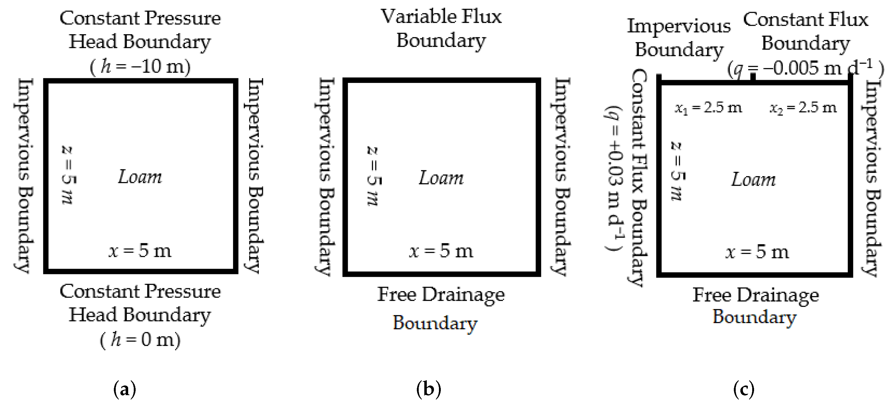
The observations are generated based on the hydraulic properties. The initial condition is set as pressure head is −10 m. The total simulation time is 120 $\mathrm{d}$, and the observation interval is 3 $\mathrm{d}$. In order to investigate the influence of boundary conditions and on the inversion results, we set up three models with three different specific boundary conditions as follows: constant pressure head boundary (Model A in Figure 2a), variable flux boundary (Model B in Figure 2b), and lateral flow boundary (Model C in Figure 2c); other parameters not mentioned can be found in Figure 2.

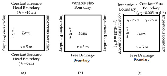
Figure 2. Schematic diagrams of the 2D section models with different boundary conditions. (a) Model A. (b) Model B. (c) Model C.

In the case of determining the coarse-scale and fine-scale grids, we want to use as few observations as possible to obtain reasonable parameter estimates, so we set up a set of different numbers of observations to investigate their effects on the inverse results. This investigation is conducted in the case of a 32 × 32 coarse-scale grid, which is a trade-off between efficiency and accuracy addressed in a later section. In the case of a coarse-scale grid of 32 × 32, if there are observations on all grids there will be 1024 observations, here we gradually and randomly reduce the number of observations by taking N equal to 1024, 974, 424, 124, 74, 24, 14, 9, 4 for nine cases.

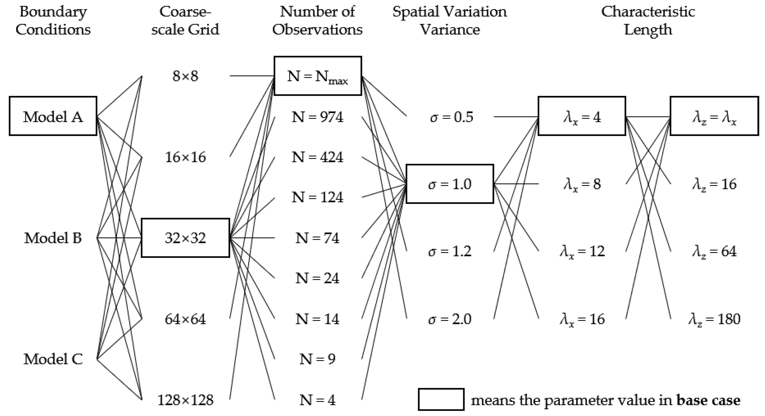
Totally, three boundary conditions and different magnitudes of decline in scale, together with different degrees of soil heterogeneity, yield to the 66 numerical experiments in this study. The combinations are shown in Figure 3.

Figure 3. Parameter and model compositions for each algorithm.

In order to measure the performance of the inverse method on these experiments, the normalized RMSE is used as a measure of agreement between observed and modeled values:

$$\begin{array}{c}\hfill \mathrm{NRMSE}=\frac{\sqrt{\frac{1}{M}{\sum }_{j=1}^M{\left({\tilde{Y}}_{\mathrm{sim}}^j-Y_{\mathrm{obs}}^j\right)}^2}}{{\tilde{Y}}_{max}-{\tilde{Y}}_{min}},\end{array}$$

(13)

where M, denotes the total number of soil water pressure head measurements or spatially distributed saturated hydraulic parameters; ${\tilde{Y}}_{\mathrm{sim}}$ and ${\tilde{Y}}_{\mathrm{obs}}$ denote the model simulated and observed value; ${\tilde{Y}}_{max}$ and ${\tilde{Y}}_{min}$ signify the maximum and minimum soil water pressure head measurement, respectively.

4. Simulation Results and Discussions

4.1. Presentation of Case Results

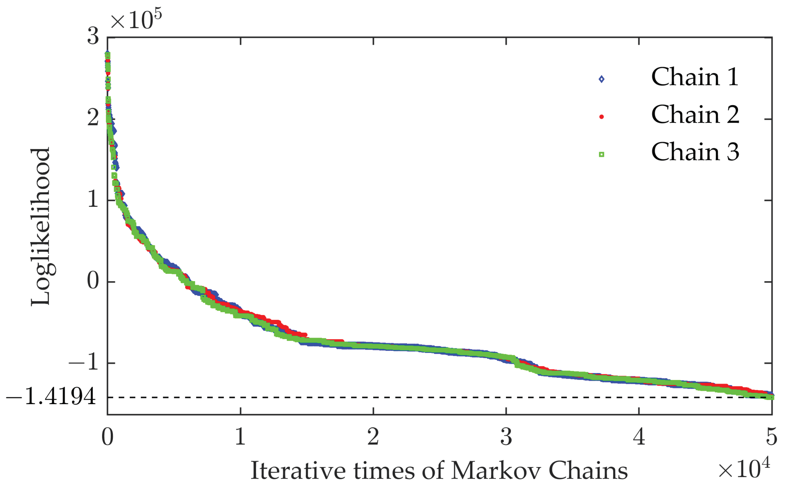
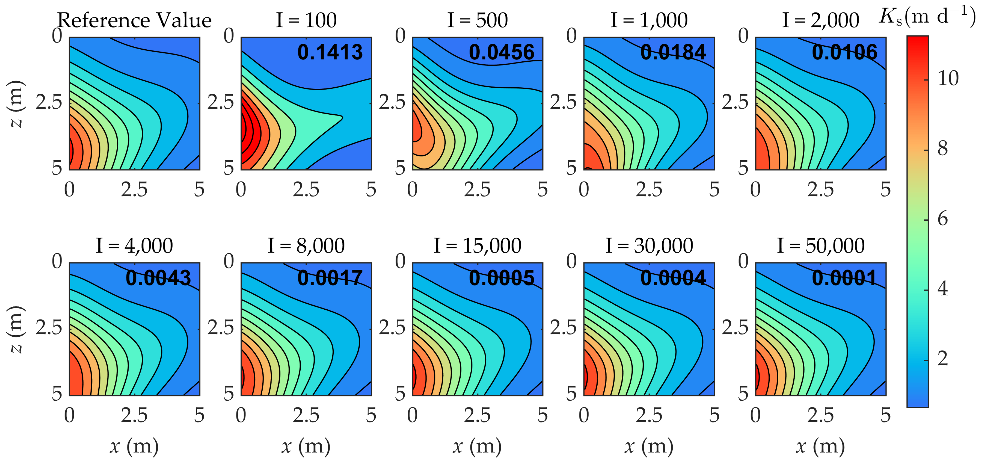
In this section we demonstrate the estimation results of saturated hydraulic conductivity by the inverse method. The results are shown here using model A as an example case, with a coarse-scale grid of 32 × 32, and spatial variability parameters $\sigma =1.0$, ${\lambda }_x={\lambda }_z=4$ m, that is, $v=1$. Figure 4 illustrates the trends of the likelihood function of the parameters to be estimated as the number of Markov chain iterations increases. The three chains show a similar convergence process, rapidly decreasing and gradually reaching the reference value of $-1.4194\times {10}^5$ during the 50,000 iterations. Given the similar convergence behavior of the three chains, we arithmetically average these chains and then plotted the averaged evolution of the estimated saturated hydraulic conductivity, as shown in Figure 5 with iteration number I =100, 500, 1000, 2000, 4000, 8000, 15,000, 30,000, 50,000. It can be seen that as the iteration number increases, the estimated and true values of the parameters match better and better, illustrated visually in the scatter plots and also in the increasingly lower values of NRMSE marked in the upper right corner.

Figure 4. The change in LogLikelihood with the iteration of the Markov chains.

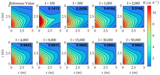
Figure 5. The change of $K_{\mathrm{s}}$ with the iteration of the Markov chains.

4.2. Effects of the Coarse- and Fine-Scale Grid Ratios

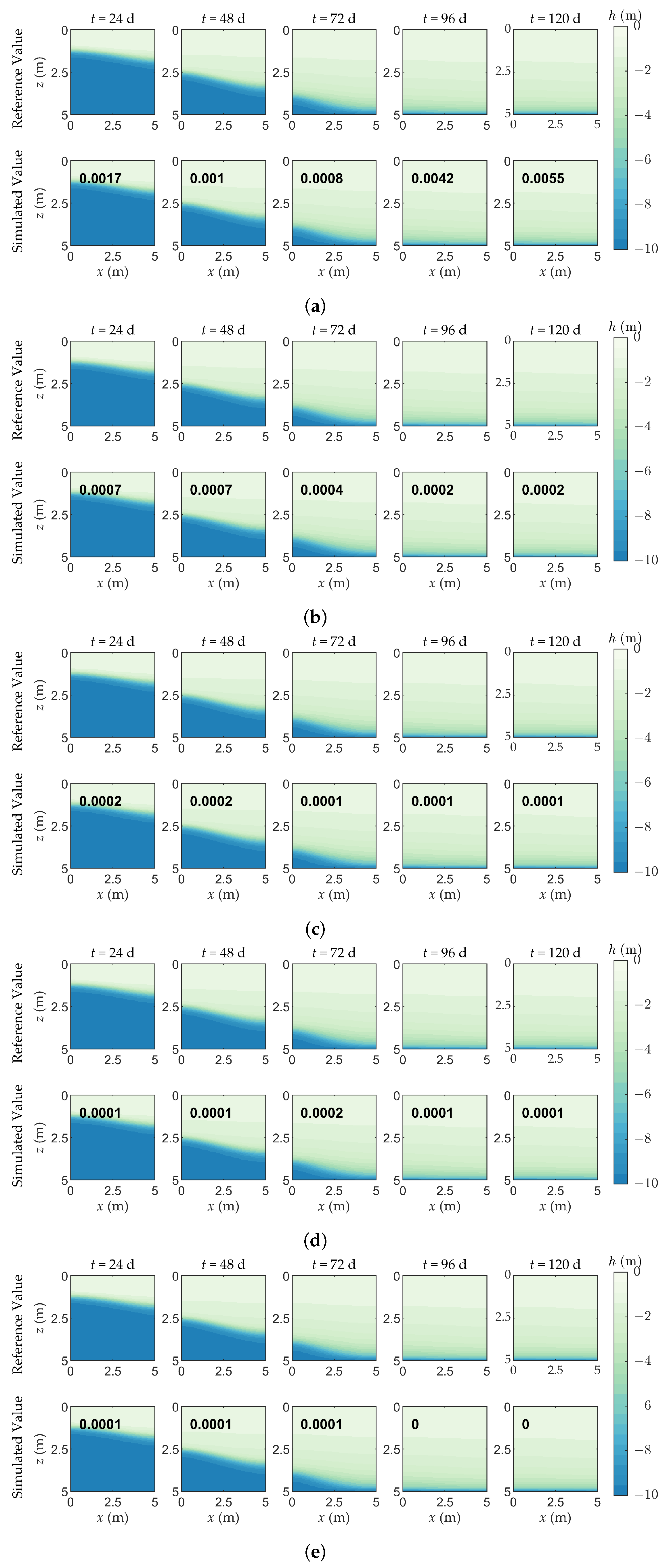
We use the case of Model A with $\sigma =1.0,{\lambda }_x={\lambda }_z=4$ m but different coarse-scale grids to illustrate the effects of the coarse- and fine-scale grid ratios on the inverse modeling. The inversely estimated saturated hydraulic conductivity fields under different coarse-scale grid are illustrated in Figure 6, and values of NRMSE are also indicated in the figure. As can be seen from the figure, all cases show good simulation results, and as the coarse-scale grid gets closer to the fine-scale grid, the simulated values match the true values more and more closely. We also show in Figure 7 the temporal and spatial distribution of soil water potential, corresponding to modeled and true saturated hydraulic conductivity fields. Overall, the estimated hydraulic conductivity is able to simulate the spatial and temporal variability of the soil water potential very well in the coarse- and fine-scale setup scenarios, as also shown by the very low NRMSE values marked in the figures.

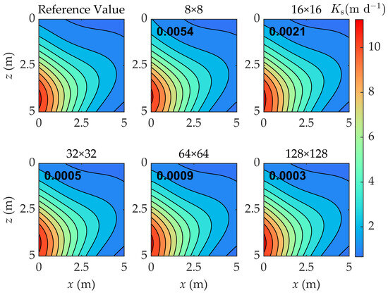
Figure 6. Comparison between the simulated and reference value of $K_{\mathrm{s}}$ field (effects of the coarse- and fine-scale grid ratios).

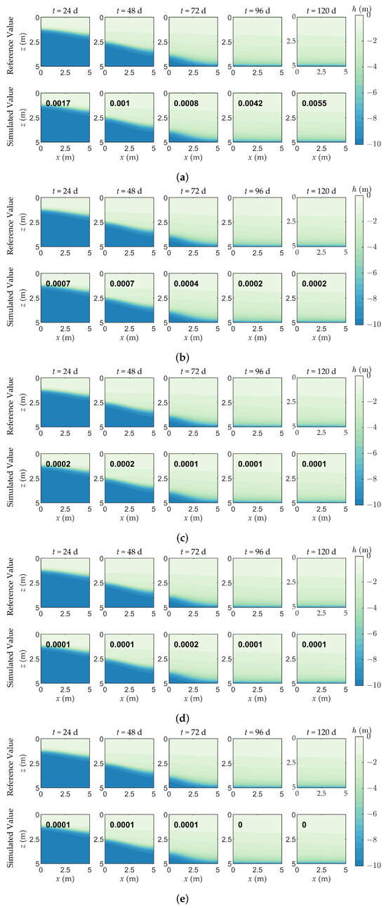
Figure 7. Comparison of reference and simulated pressure head values (effects of the coarse- and fine-scale grid ratios). (a) 8 × 8. (b) 16 × 16. (c) 32 × 32. (d) 64 × 64. (e) 128 × 128.

Table 1 further gives the time spent on the inversion and the values of the evaluation metrics for different coarse-scale grids. As can be seen, when a fine-scale grid is determined as 128 × 128, the greater the difference between the coarse and fine-scales, the lower the cost of the observation and the less the inverse simulation consumes, but also the lower the accuracy of the reconstruction of the fine-scale saturated hydraulic conductivity. Therefore, we need to make a trade-off between accuracy and cost.

Table 1. The simulation time with $K_{\mathrm{s}}$-NRMSE at different scales in Model A.

Scale	Simulation Time (min)	${\mathit{K}}_{\mathbf{s}}$-NRMSE
8 × 8	59	0.0054
16 × 16	89	0.0021
32 × 32	178	0.0005
64 × 64	534	0.0009
128 × 128 (fine-scale)	1067	0.0003

Through the above analyses, in the research situation of this paper, the coarse grid taking the size of 32 × 32 to 64 × 64 are more appropriate choices, which can guarantee a certain computational accuracy at the same time, the computational efficiency will be increased to 2 to 6 times of the original, which is why the other calculations of this paper set the size of its coarse grid to 32 × 32. Due to limitations on the length of the paper, the results related to model B and C are not represented graphically, but list metrics in Table 2 only.

Table 2. Variation in the NRMSE with the scale size for the simulated and the reference $K_{\mathrm{s}}$.

Model	Scale Size (NRMSE)
	8 × 8	16 × 16	32 × 32	64 × 64	128 × 128
A	0.0054	0.0021	0.0005	0.0009	0.0003
B	0.0640	0.0174	0.0023	0.0005	0.0002
C	0.0317	0.0988	0.0452	0.0334	0.0431

4.3. Effects of the Spatial Distribution of the $K_{\mathrm{s}}$ Field

The spatial distribution of the $K_{\mathrm{s}}$ field is expressed using three statistic parameters: spatial variation variance, characteristic length and anisotropy ratio. This section conducts numerical simulations in either isotropic ($\lambda ={\lambda }_x$ = ${\lambda }_z$ = 8, 12, 16 m) or anisotropic (${\lambda }_x$ = 4 m, ${\lambda }_z$ = 16, 64, 180 m, that is, v = 4, 16, 45) soil profiles with $\sigma$ = 0.5, 1.2, 2.0.

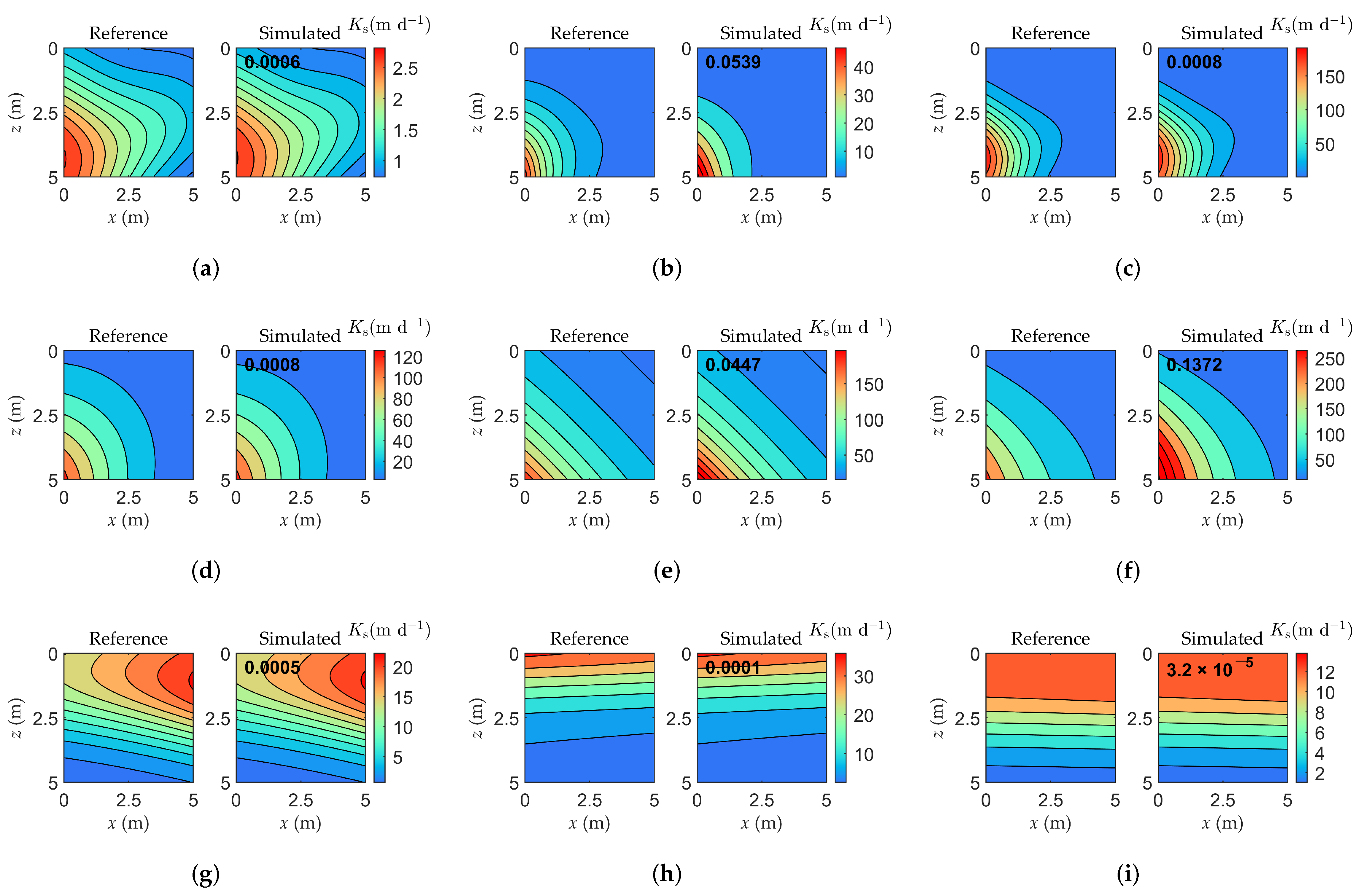
The inverse results under different soil heterogeneity conditions are illustrated in Figure 8. Because previous figures has shown the case with $\sigma =1.0,{\lambda }_x={\lambda }_z$ = 4 m, here, results only under other conditions are illustrated. The quantitative metrics are listed in Table 3 using NRMSE. From the figure, it can be observed that overall the inversion effect has a tendency to become better as the spatial variability of the $K_{\mathrm{s}}$ field becomes smaller.

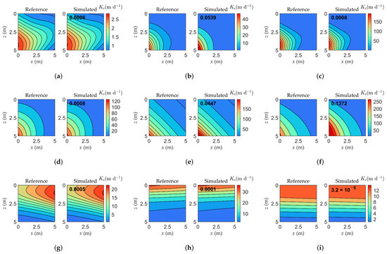
Figure 8. Comparison between the simulated and reference value of $K_{\mathrm{s}}$ (effects of the spatial distribution of the $K_{\mathrm{s}}$ Field). (a) $\sigma$ = 0.5. (b) $\sigma$ = 1.2. (c) $\sigma$ = 2. (d) $\lambda$ = 8. (e) $\lambda$ = 12. (f) $\lambda$ = 16. (g) v = 4. (h) v = 16. (i) v = 45.

Table 3. Variation in the NRMSE with the number of observation points for the simulated $K_{\mathrm{s}}$ and the reference $K_{\mathrm{s}}$.

Model	Number of Observation Points (NRMSE)
	$\mathit{\sigma }$ = 0.5	$\mathit{\sigma }$ = 1.2	$\mathit{\sigma }$ = 2.0	$\mathit{\lambda }$ = 8	$\mathit{\lambda }$ = 16	$\mathit{\lambda }$ = 32	$\mathit{v}$ = 4	$\mathit{v}$ = 16	$\mathit{v}$ = 45
A	0.0006	0.0539	0.0008	0.0008	0.0447	0.1372	0.0005	0.0001	3.20 × 10−5
B	0.0024	0.0008	0.0095	4.85 $\times {10}^{-5}$	1.19 $\times {10}^{-5}$	2.95 $\times {10}^{-6}$	0.0001	1.05 $\times {10}^{-5}$	2.51 $\times {10}^{-6}$
C	0.0785	0.0056	0.0092	0.0084	0.0010	0.0006	0.0393	0.0296	0.0165

4.4. Impact of Observation Site Density

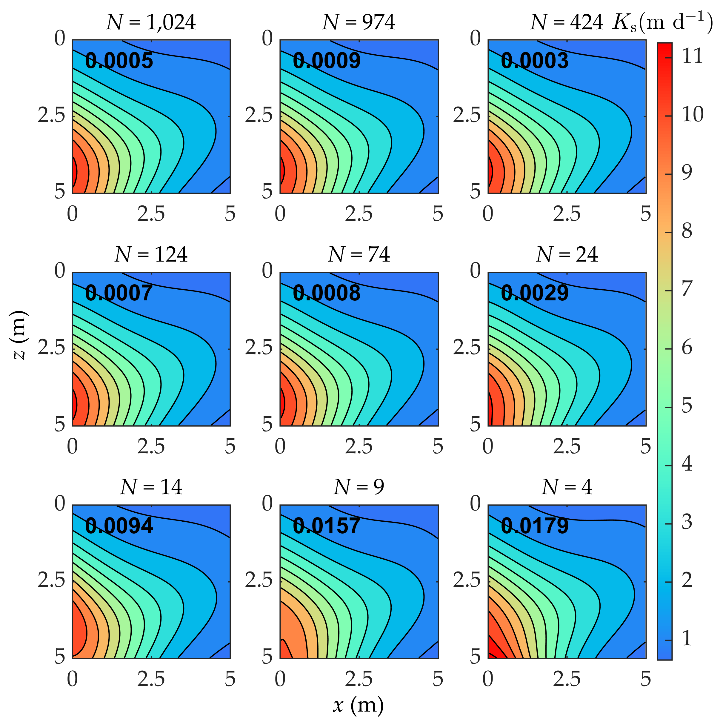
In the case of a coarse-scale grid of 32 × 32 (1024 observations), we gradually and randomly reduce the number of observations to obtain nine cases of N = 1024, 974, 424, 124, 74, 24, 14, 9, 4. Figure 9 depicts the plots of the simulated values of the $K_{\mathrm{s}}$ field against the reference values for these cases with the boundary condition denoted Model A. It can be observed that the values of NRMSE are stable around a small value for all the cases where the N value of the total number of actual observation points is above 74. That is, when the number of observations is greater than or equal to 7% of the total grid, a very satisfactory agreement between the estimated and true values is obtained, and when the number of observations is less than 7% of the total grid, the gap between the simulated and real values gradually becomes larger. We also conduct the investigation with other two boundary conditions denoted Model B and C, and the corresponding results are shown in Table 4.

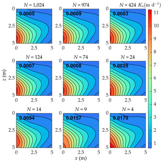
Figure 9. Comparison between the simulated and reference value of $K_{\mathrm{s}}$ field (impact of observation site density).

Table 4. Variation in the NRMSE with the spatial distribution for the simulated $K_{\mathrm{s}}$ and the reference $K_{\mathrm{s}}$.

Model	Spatial Distribution of ${\mathit{K}}_{\mathit{s}}$ Field (NRMSE)
	$\mathit{N}$ = 974	$\mathit{N}$ = 424	$\mathit{N}$ = 124	$\mathit{N}$ = 74	$\mathit{N}$ = 24	$\mathit{N}$ = 14	$\mathit{N}$ = 9	$\mathit{N}$ = 4
A	0.0009	0.0003	0.0007	0.0008	0.0029	0.0094	0.0157	0.0179
B	0.0058	0.0045	0.0029	0.0031	0.0017	0.0037	0.0026	0.0313
C	0.0169	0.0244	0.0445	0.0882	0.0763	0.0105	0.0079	0.0178

5. Conclusions

In this paper, for the spatially characterizing high-resolution soil saturated hydraulic conductivity, a multiscale dynamic data integration method is proposed to obtain these parameters on finer scales based on the inversion of dynamic observations on coarse scales. The method uses Bayesian statistical inference as the inversion framework, combines an analytical upscaling method and KL expansion, constructs a posteriori distributions of saturated hydraulic parameters based on observations on coarse scales, and performs sampling simulations of the posteriori distributions to reconstruct the parameter fields at high resolution. The method provides an effective solution to the computational efficiency, scale integration, and parameter uncertainty problems of multiscale inversions, and is demonstrated and validated in a series of numerical experiments. The numerical results show that the proposed method has good applicability for different boundary conditions, and is very tolerant to large-scale variability in soil heterogeneity. The performance of the proposed method corresponding to the coarse- and fine-scale grid setup indicated that the method can be used to integrate data from different coarse scales as well as coarse scales that differ significantly from fine scales.

References

- Rallo, G.; Provenzano, G.; Castellini, M.; Sirera, À.P. Application of EMI and FDR sensors to assess the fraction of transpirable soil water over an olive grove. Water 2018, 10, 168. [Google Scholar] [CrossRef]
- Sanayei, H.R.Z.; Talebdokhti, N.; Rakhshandehroo, G.R. Analytical solutions for water infiltration into unsaturated–semi-saturated soils under different water content distributions on the top boundary. Iran. J. Sci. Technol. Trans. Civ. Eng. 2019, 43, 747–760. [Google Scholar] [CrossRef]
- Liu, S.; Fan, M.; Lu, D. Uncertainty quantification of the convolutional neural networks on permeability estimation from micro-CT scanned sandstone and carbonate rock images. Geoenergy Sci. Eng. 2023, 230, 212160. [Google Scholar] [CrossRef]
- Savvides, A.A.; Papadrakakis, M. Uncertainty Quantification of Failure of Shallow Foundation on Clayey Soils with a Modified Cam-Clay Yield Criterion and Stochastic FEM. Geotechnics 2022, 2, 348–384. [Google Scholar] [CrossRef]
- Hmimou, A.; Maslouhi, A.; Tamoh, K.; Candela, L. Experimental monitoring and numerical study of pesticide (carbofuran) transfer in an agricultural soil at a field site. Comptes Rendus Geosci. 2014, 346, 255–261. [Google Scholar] [CrossRef]
- Qanza, H.; Maslouhi, A.; Hachimi, M.; Hmimou, A. Inverse estimation of the hydrodispersive properties Of unsaturated soil using complex-variable-differentiation method under field experiments conditions. Eurasian Soil Sci. 2018, 51, 1229–1239. [Google Scholar] [CrossRef]
- Rezaei, M.; Seuntjens, P.; Joris, I.; Boënne, W.; Van Hoey, S.; Campling, P.; Cornelis, W. Sensitivity of water stress in a two-layered sandy grassland soil to variations in groundwater depth and soil hydraulic parameters. Hydrol. Earth Syst. Sci. 2016, 20, 487–503. [Google Scholar] [CrossRef]
- Qanza, H.; Maslouhi, A.; Abboudi, S. Experience of inverse modeling for estimating hydraulic parameters of unsaturated soils. Russ. Meteorol. Hydrol. 2016, 41, 779–788. [Google Scholar] [CrossRef]
- Lin, Q.; Xu, S. Parameter identification and uncertainty analysis of soil water movement model in field layered soils based on Bayes Theory. J. Hydraul. Eng. 2018, 49, 428–438. [Google Scholar] [CrossRef]
- Yu, M.; Zhang, K. Identification of soil hydraulic parameters based on HYDRUS-2D software and simulation of soil water movement under indirect subsurface drip irrigation. Acta Agric. Zhejiangensis 2019, 31, 458–468. [Google Scholar] [CrossRef]
- Brunetti, G.; Šimůnek, J.; Bogena, H.; Baatz, R.; Huisman, J.A.; Dahlke, H.; Vereecken, H. On the information content of cosmic-ray neutron data in the inverse estimation of soil hydraulic properties. Vadose Zone J. 2019, 18, 1–24. [Google Scholar] [CrossRef]
- Mustapha, H.; Abdellatif, M.; Karim, T.; Hamid, Q. Estimation of soil hydraulic properties of basin Loukkos (Morocco) by inverse modeling. KSCE J. Civ. Eng. 2019, 23, 1407–1419. [Google Scholar] [CrossRef]
- Pan, M.; Huang, Q.; Feng, R.; Huang, G. Estimation of water and heat transfer parameters of saturated silica sand by using different types of data. Trans. Chin. Soc. Agric. Eng. 2020, 36, 75–82. [Google Scholar] [CrossRef]
- Zhao, Z.; Illman, W.A. Improved high-resolution characterization of hydraulic conductivity through inverse modeling of HPT profiles and steady-state hydraulic tomography: Field and synthetic studies. J. Hydrol. 2022, 612, 128124. [Google Scholar] [CrossRef]
- Bandai, T.; Ghezzehei, T.A. Forward and inverse modeling of water flow in unsaturated soils with discontinuous hydraulic conductivities using physics-informed neural networks with domain decomposition. Hydrol. Earth Syst. Sci. 2022, 26, 4469–4495. [Google Scholar] [CrossRef]
- Singh, U.; Sharma, P.K. Comparison of saturated hydraulic conductivity estimated by surface NMR and empirical equations. J. Hydrol. 2023, 617, 128929. [Google Scholar] [CrossRef]
- Vrugt, J.A.; Ter Braak, C.J.; Clark, M.P.; Hyman, J.M.; Robinson, B.A. Treatment of input uncertainty in hydrologic modeling: Doing hydrology backward with Markov chain Monte Carlo simulation. Water Resour. Res. 2008, 44. [Google Scholar] [CrossRef]
- Vrugt, J.A.; ter Braak, C.J.; Diks, C.G.; Robinson, B.A.; Hyman, J.M.; Higdon, D. Accelerating Markov chain Monte Carlo simulation by differential evolution with self-adaptive randomized subspace sampling. Int. J. Nonlinear Sci. Numer. Simul. 2009, 10, 273–290. [Google Scholar] [CrossRef]
- Laloy, E.; Vrugt, J.A. High-dimensional posterior exploration of hydrologic models using multiple-try DREAM (ZS) and high-performance computing. Water Resour. Res. 2012, 48. [Google Scholar] [CrossRef]
- Vrugt, J.A. Markov chain Monte Carlo simulation using the DREAM software package: Theory, concepts, and MATLAB implementation. Environ. Model. Softw. 2016, 75, 273–316. [Google Scholar] [CrossRef]
- Jiang, S.; Jomaa, S.; Büttner, O.; Meon, G.; Rode, M. Multi-site identification of a distributed hydrological nitrogen model using Bayesian uncertainty analysis. J. Hydrol. 2015, 529, 940–950. [Google Scholar] [CrossRef]
- Jiang, S.; Yuan, L.; Zhang, X.; Huang, J.; Zhou, C. Stochastic back analysis and comparison of spatially varying geotechnical mechanical parameters based on limited data. Chin. J. Rock Mech. Eng. 2020, 39, 1265–1276. [Google Scholar] [CrossRef]
- Morandage, S.; Laloy, E.; Schnepf, A.; Vereecken, H.; Vanderborght, J. Bayesian inference of root architectural model parameters from synthetic field data. Plant Soil 2021, 467, 67–89. [Google Scholar] [CrossRef]
- Liu, Y.; Fernández-Ortega, J.; Mudarra, M.; Hartmann, A. Pitfalls and a feasible solution for using KGE as an informal likelihood function in MCMC methods: DREAM (ZS) as an example. Hydrol. Earth Syst. Sci. 2022, 26, 5341–5355. [Google Scholar] [CrossRef]
- Guo, Q.; Wu, W. Application of parameter optimization methods based on Kalman formula to the soil–crop system model. Int. J. Environ. Res. Public Health 2023, 20, 4567. [Google Scholar] [CrossRef] [PubMed]
- Li, N.; Yue, X.; Ren, L. Numerical homogenization of the Richards equation for unsaturated water flow through heterogeneous soils. Water Resour. Res. 2016, 52, 8500–8525. [Google Scholar] [CrossRef]
- Zhu, J.; Mohanty, B.P. Spatial averaging of van Genuchten hydraulic parameters for steady-state flow in heterogeneous soils: A numerical study. Vadose Zone J. 2002, 1, 261–272. [Google Scholar] [CrossRef]
- Zhu, J.; Mohanty, B.P. Effective hydraulic parameters for steady state vertical flow in heterogeneous soils. Water Resour. Res. 2003, 39. [Google Scholar] [CrossRef]
- Zhu, J.; Mohanty, B. Upscaling of hydraulic properties of heterogeneous soils. In Scaling Methods in Soil Physics; Routledge: Abingdon, UK, 2003; pp. 97–118. [Google Scholar] [CrossRef]
- Roth, K.; Vogel, H.; Kasteel, R. The scaleway: A conceptual framework for upscaling soil properties. In Modelling of Transport Processes in Soils; Wageningen Pers: Wageningen, The Netherlands, 1999; pp. 477–490. Available online: https://citeseerx.ist.psu.edu/document?repid=rep1&type=pdf&doi=4653aa13563ead62a92b8a9d0dc56dcea32b232d (accessed on 15 May 2024).
- Vogel, H.J.; Roth, K. Moving through scales of flow and transport in soil. J. Hydrol. 2003, 272, 95–106. [Google Scholar] [CrossRef]
- Li, N.; Yue, X.; Wang, W.; Ma, Z. Inverse estimation of spatiotemporal flux boundary conditions in unsaturated water flow modeling. Water Resour. Res. 2021, 57, e2020WR028030. [Google Scholar] [CrossRef]
- Comunian, A.; Giudici, M. Hybrid inversion method to estimate hydraulic transmissivity by combining multiple-point statistics and a direct inversion method. Math. Geosci. 2018, 50, 147–167. [Google Scholar] [CrossRef]
- Lan, T.; Shi, X.; Jiang, B.; Sun, Y.; Wu, J. Joint inversion of physical and geochemical parameters in groundwater models by sequential ensemble-based optimal design. Stoch. Environ. Res. Risk Assess. 2018, 32, 1919–1937. [Google Scholar] [CrossRef]
- Wuwen, Q.; Junrui, C.; Yuan, Q.; Zengguang, X. Simulation-optimization model for estimating hydraulic conductivity: A numerical case study of the Lu Dila hydropower station in China. Hydrogeol. J. 2019, 27, 2595–2616. [Google Scholar] [CrossRef]
- Uribe, F.; Papaioannou, I.; Betz, W.; Straub, D. Bayesian inference of random fields represented with the Karhunen–Loève expansion. Comput. Methods Appl. Mech. Eng. 2020, 358, 112632. [Google Scholar] [CrossRef]
- Blaheta, R.; Béreš, M.; Domesová, S.; Horák, D. Bayesian inversion for steady flow in fractured porous media with contact on fractures and hydro-mechanical coupling. Comput. Geosci. 2020, 24, 1911–1932. [Google Scholar] [CrossRef]
- Gu, X.; Wang, L.; Ou, Q.; Zhang, W.; Sun, G. Reliability assessment of rainfall-induced slope stability using Chebyshev-Galerkin-KL expansion and Bayesian approach. Can. Geotech. J. 2023, 60, 1909–1922. [Google Scholar] [CrossRef]
- Mualem, Y. A new model for predicting the hydraulic conductivity of unsaturated porous media. Water Resour. Res. 1976, 12, 513–522. [Google Scholar] [CrossRef]
- Van Genuchten, M.T. A closed-form equation for predicting the hydraulic conductivity of unsaturated soils. Soil Sci. Soc. Am. J. 1980, 44, 892–898. [Google Scholar] [CrossRef]
Disclaimer/Publisher’s Note: The statements, opinions and data contained in all publications are solely those of the individual author(s) and contributor(s) and not of MDPI and/or the editor(s). MDPI and/or the editor(s) disclaim responsibility for any injury to people or property resulting from any ideas, methods, instructions or products referred to in the content. |
© 2024 by the authors. Licensee MDPI, Basel, Switzerland. This article is an open access article distributed under the terms and conditions of the Creative Commons Attribution (CC BY) license (https://creativecommons.org/licenses/by/4.0/).