A Deep Learning Method to Mitigate the Impact of Subjective Factors in Risk Estimation for Machinery Safety

Abstract

Risk estimation holds significant importance in the selection of risk reduction measures and ensuring machinery safety. However, subjective influences of assessors lead to an inconsistent understanding of risk among relevant stakeholders, hindering the achievement of safety. As similarities exists in product updates or applications in engineering practice, the historical risk information of similar products or applications has essential application value. A novel deep learning approach was established to estimate risks based on historical risk information. To address the issue of overfitting caused by a limited dataset, a data augmentation technique was employed. Our experiment was conducted on the raw, 2×, and 6× hazard event dataset of an industrial robot, demonstrating a substantial improvement in both accuracy and stability. On the validation dataset, there was an increase in median accuracy from 55.56% to 96.92%, with a decrease in standard deviation from 0.118 to 0.015. On the new dataset, the trained network also showed near-perfect performance on similar hazard events and trustworthiness on completely different ones. In cases of risk deviations, approximately 80% of them were small deviations (|RI_deviation| ≤ 2) without a noticeable bias (RI_dis is close to 1). The LSTM-based deep learning network makes risk estimation “black-boxed” and “digitized”. Assessors just need to focus on hazard identification with risk being determined by the trained network, mitigating the impact of individual factors. Moreover, the historical risk estimation information can be transformed into a trained network, facilitating the development of a standardized benchmark within project teams, enterprises, and relevant stakeholders to promote coordinated safety measures.

1. Introduction

Machinery/machines are assembled, fitted with or intended to be fitted with a drive system consisting of linked parts or components, at least one of which moves, and which are joined together for a specification [1]. The manufacturer of machinery or his authorized representative is mandated by Directive 2006/42/EC Annex I to ensure that a risk assessment is carried out in order to determine the health and safety requirements that apply to the machinery, and the machinery must then be designed and constructed taking into account the results of the risk assessment [2]. Safety standards for industrial robots [3], collaborative robots [4], robot systems and integration [5], etc., clearly stipulate the technical requirements of hazard identification and risk assessment. Reference [1] specifies procedures of risk assessment and risk reduction to achieve safety in the design of machinery. After hazard identification, risk estimation is conducted for each identified hazard event/situation.

The estimated risk level bears significant implications for the selection of hazard reduction measures and the ensuring of machine safety. The overestimation of the risk might lead to excessive machine safety design, thereby inflating costs. Conversely, insufficient risk estimation could compromise the safety of product design and inadvertently trigger dangers. Product standards usually specify Performance Level (PL) or Safety Integrity Level (SIL) requirements for their safety functions [3,5,6,7]. If no product-related standards exist, the determination of the required performance level PLr for each safety function can be carried out by a risk estimation approach [8,9], while reference [10] estimates the required SIL. Excessive dispersion in the risk estimation results may lead to inappropriate risk reduction measures being implemented [8].

Risk is relevant to the severity of harm and the probability of the occurrence of that severity of harm. In the process of risk estimation, each risk element is generally divided into several discrete grades or scores, and then the risk assessors select the grade or acquire the score by qualitative or quantitative approaches. The final risk level is obtained through risk estimation tools or methods, such as a risk matrix, risk graph, numerical scoring and hybrid tools using a combination of methods [11]. Reference [12] notes that machinery-related risk estimation is mainly based on qualitative and static tools, which lead to subjective decision-making. The influence of subjective factors on the results of risk estimation primarily comes from the following three aspects:

• The definitions or descriptions of scaled risk elements typically employ qualitative or a combination of qualitative and quantitative textual descriptions, leading to disparate interpretations. For example, reference [11] suggests that the severity of the harm S can be classified as: S1-slight injury, and S2-serious injury. Understanding those descriptions is very subjective and there tends to be significant variation between different risk assessment members [13]. Given that risk assessments pertain to potential future scenarios, such statements are intrinsically uncertain, by virtue of their inherent nature, and it is not easy to define scales unambiguously by mostly using nominal and textual descriptions. Reference [14] shared an experience in which subjects had to allocate a quantitative value to the verbal labels of probability, and concluded that regardless of whether the verbal labels were detailed, the probability assigned would vary due to distinct interpretations.
• Risk assessment members’ characteristics. The familiarity with the machine, background, and position of the persons who performed the risk assessment, and other factors such as optimism bias, confirmation bias, and overconfidence will affect the judgement of likelihood and consequence; the most significant divergence was detected in the estimation of the parameter Fr (frequency and duration of exposure) [8]. Subject to fluctuations in fatigue levels, mood, etc., the same individual may make different risk estimation results at different times, known as individual variability [14]. In addition, risk aversion also impacts risk estimation outcomes, which can be interpreted as an attitude that assigns a higher risk value to a low-probability, high-consequence event compared to a high-probability, low-consequence event, even when the expected loss for both events is the same [15].
• Insufficient data or unlimited resources are often available to support estimating the risk objectively. To conduct risk estimation, assessors need to choose one class for each parameter that best corresponds to the hazardous situation. Those choices are best made by a quantitative method; however, reference [1] notes that a quantitative approach to risk estimation is restricted by the valuable data that are available and/or the limited resources. Reference [16] thought that not all potential risk factors could be considered due to the restrictions associated with publicly available occupational injury data, and the absence of enough historical accident cases. Assessments of likelihood and consequence of adverse events are usually not precise, but rather subjective estimations that, due to the infrequent nature of the events, can seldom be verified against observations or statistics [13].

2. Related Works

Significant efforts have been carried out by researchers to improve risk estimation:

• Focus on the advancement of risk matrices and the optimization of risk estimation tools. Reference [16] took additional severity factors into consideration, including employee factors, workspace factors, worksite location, etc., and proposed the Accident Severity Grade (ASG) method based on employee and workspace risk factors to quantify the injury risk. Reference [17] proposed a three-dimensional risk assessment matrix—injury frequency, severity, and the new dimension—preventability, to improve risk estimation. Reference [18] developed a proposed risk estimation tool with five risk parameters, severity of harm, frequency of exposure to the hazard, duration of exposure to the hazard, probability of occurrence of a hazardous event, possibility of avoidance. However, given that risk estimation is an intricate and extensive cognitive process, it is unavoidable that the subjective factors of risk assessors have a bearing on the results of risk estimation.
• With the development of AI, machine learning techniques are also finding their way into the field of safety [19]. Paltrinieri, Comfort et al. used a Deep Neural Network (DNN) model to predict risk increase or decrease as the target system conditions changed [20]. Natural language-based probabilistic risk assessment models applying deep learning algorithms were developed to emulate experts’ quantified risk estimates, which allowed the risk analyst to obtain an a priori risk assessment [21].
• Authors have made recommendations and proposed other tools or other methods. Jocelyn, Chinniah et al. integrated a Logical Analysis of Data (LAD)-based dynamic experience feedback into quantitative risk estimation to identify and update the risks, guiding safety practitioners to evaluate whether the current state of machine leads to an accident or not [22]. Bayesian networks (BN) and a Fuzzy Bayesian Network (FBN) were applied for predictive analysis and probability updating to improve risk assessment [23,24]. Those methods were based on strong models and little data, leading to large sets of assumptions and simulations for their environment.

The research mentioned above has significantly contributed to enhancing risk estimation practices. However, it is unavoidable that the subjective factors of risk assessors have a bearing on the results of risk estimation. It is also challenging to build a uniform benchmark for risk estimation, causing disagreements over the risk estimation results. Reference [25] observed that in several other companies, a standard corporate risk matrix for risk estimation shall be applied to both continuous operations and construction and maintenance projects. In addition, throughout the utilization of machinery, it is challenging for manufacturers, users, integrators, and other stakeholders to establish a consensus on safety awareness because of the disagreements, which hampers the collaborative implementation of more effective risk reduction measures by all parties.

In this study, a deep learning algorithm, Long Short-Term Memory(LSTM) [26], was introduced to learn and use those historical risk estimation information. This article is organized as follows: In Section 3 (Materials and Methods), the comprehensive framework of the methodology, how to create hazard event dataset, and the principle of LSTM-based risk estimation algorithm are presented. The following section, Section 4 (Results) validates the new risk estimation methodology on the raw, 2×, and 6× hazard event dataset of industrial robot. Section 5 (Discussion) briefly discusses the performance of the LSTM-based deep learning risk estimation method, and Section 6 (Conclusions) presents the conclusion.

3. Materials and Methods

3.1. The Comprehensive Framework of LSTM-Based Risk Estimation Methodology

The comprehensive framework of LSTM-based risk estimation methodology is shown in Figure 1, which can be essentially divided into two major stages: (a) create a LSTM-based deep learning network and train the network utilizing the historical hazard event dataset, as shown by the light blue node in the figure; (b) input a new hazard event, use the trained network to estimate its risk, and obtain the risk index of the new hazard event, as shown by the purple node in Figure 1. The detailed procedures are as follows:

Stage (a) Create and train the LSTM-based deep learning network:

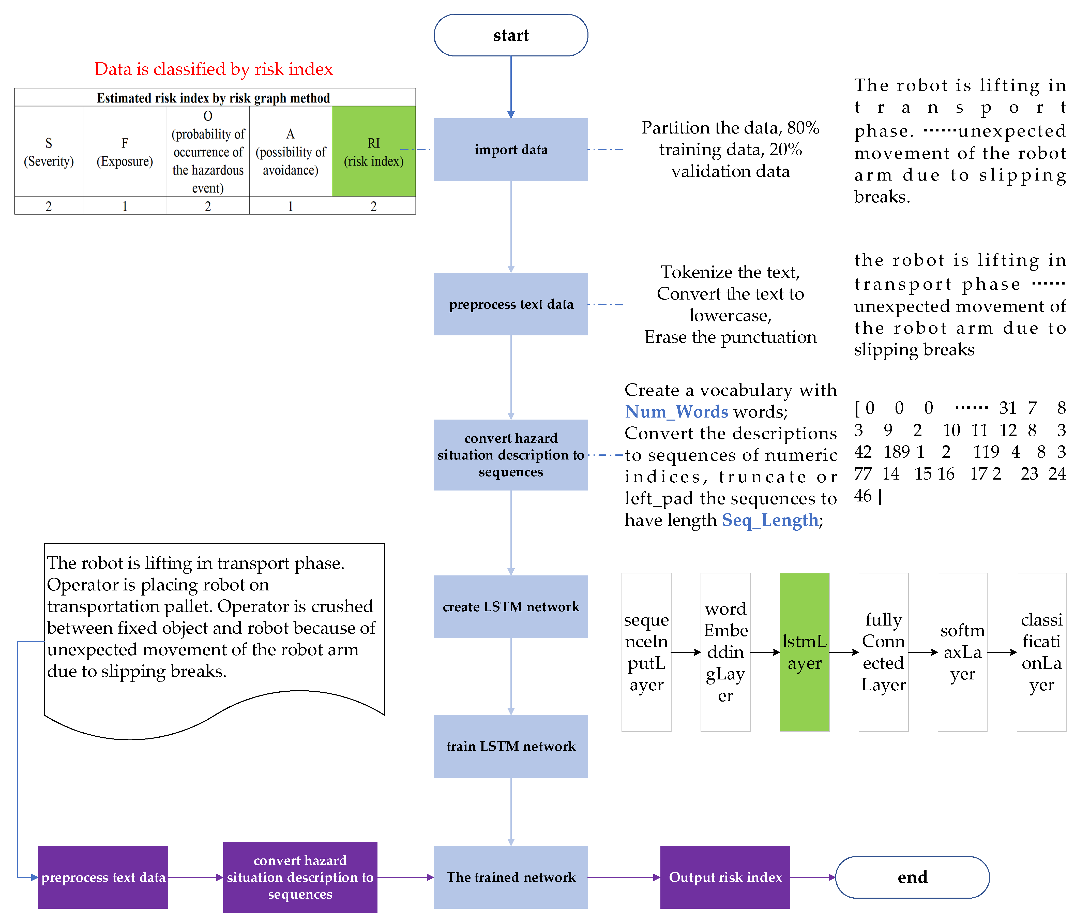
• Import the historical hazard event dataset into the network. Each hazard event is the combination of a hazardous situation description and the corresponding risk index. The dataset is partitioned into two parts, with a certain proportion of the data being used as the training set and a held-out proportion for validation. Since each hazardous situation description is associated with a corresponding risk index, the risk estimation task can be considered a classification of hazardous situation descriptions based on risk indices.
• Preprocess the hazardous situation description text to facilitate further processing, including tokenizing the text, converting the text to lowercase, and erasing punctuation.
• Convert the hazardous situation descriptions text into sequences. The textual descriptions of hazardous situations cannot be processed by the computer, which must be digitalized to generate vector data that the computer can process. In this step, a vocabulary dictionary is constructed upon the training data, with the serial number of each word in the dictionary being assigned.
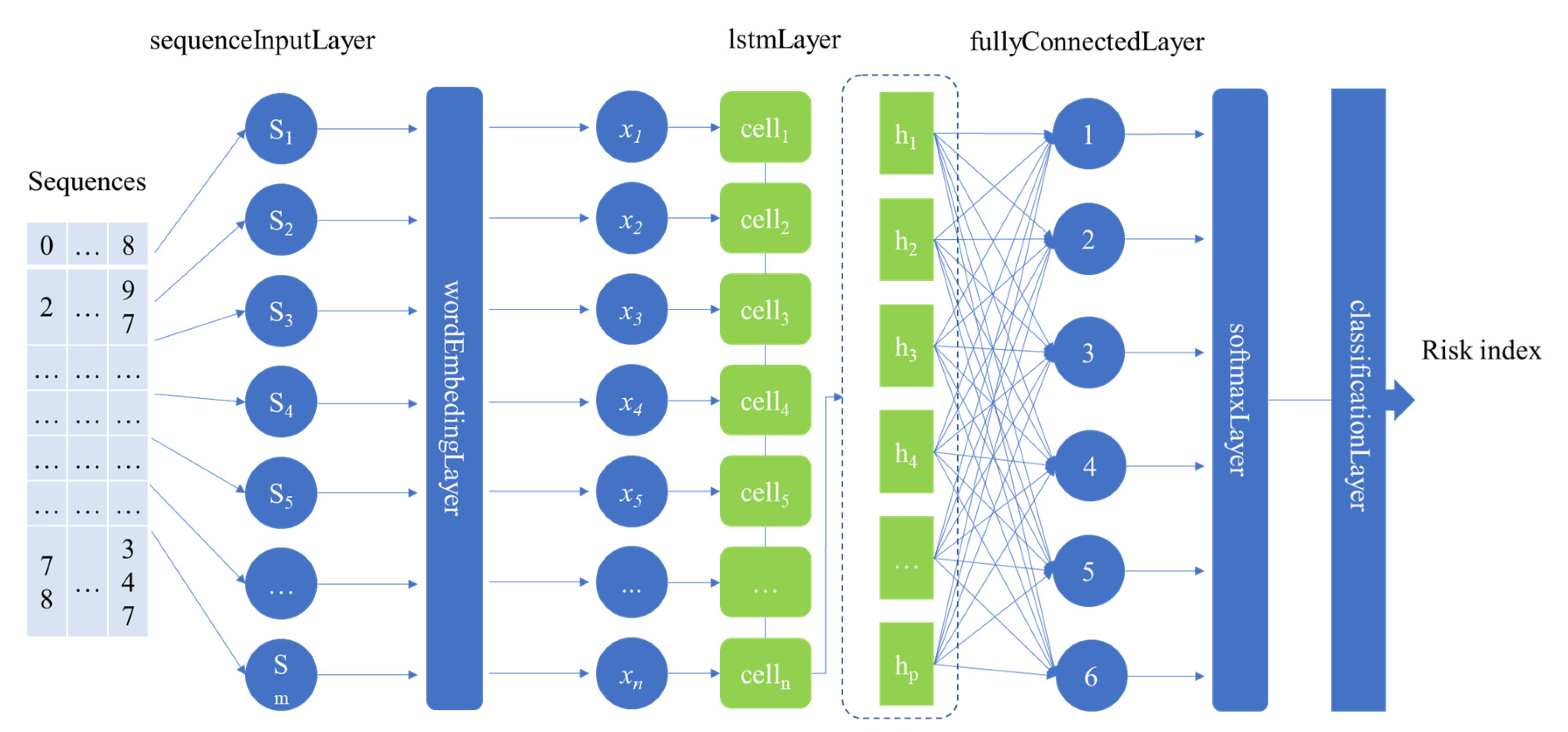
• Create the LSTM-based deep learning network with six layers, including sequenceInputLayer, wordEmbeddingLayer, lstmLayer, fullyConnectedLayer, softmaxLayer, and classificationLayer. The function of each layer in the network is described in Section 3.3.2.
• Training the network by historical risk events dataset, and the weight parameters of the network are updated to obtain the trained network.

Stage (b) Estimate the risk of new hazard events by the trained network:

6.

For new hazard events, repeat 2 and 3, then input the processed data into the trained network to obtain the risk indices for the hazard events.

7.

Output risk indices and complete the risk estimation of new hazard events.

3.2. Creating Hazard Event Dataset

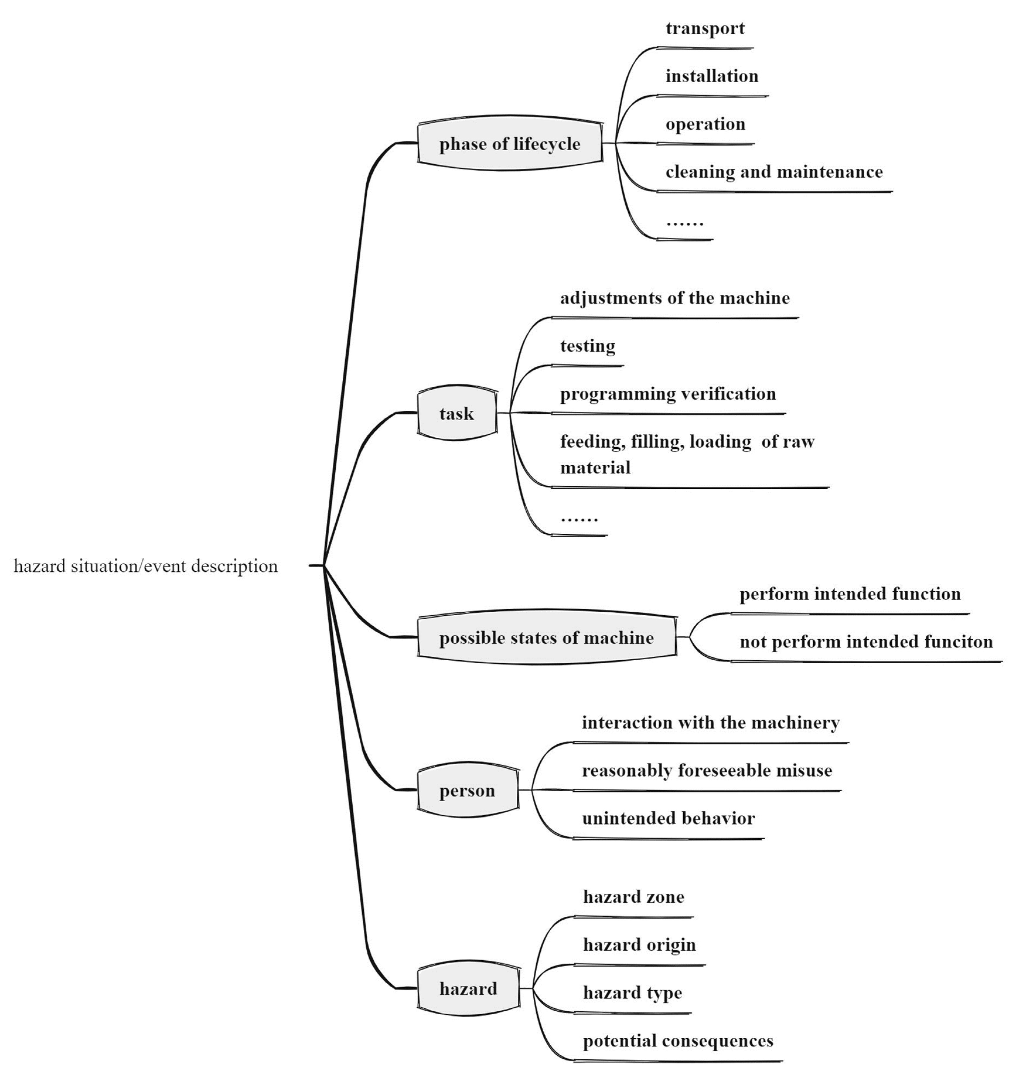
3.2.1. Elements of Hazardous Situation Description

The hazard event dataset mentioned in this paper was a set of hazardous situation descriptions combined with their corresponding risk indices. A hazard event refers to an event that can cause harm [27], which is determined by risk identification according to [1] and generally described by a paragraph of text. The description of a hazard event is crucial for the risk estimation, which should incorporate sufficient information to determine various risk elements. The absence of crucial hazardous situation description elements may pose significant challenges to the risk estimation process and render the selection of appropriate risk levels more difficult.

To aid risk assessment members in estimating the risk level, the description of the hazard event should incorporate, to the greatest extent possible, the considerations taken in risk identification (e.g., limitations on machinery use) and the elements requiring elucidation in risk estimation (e.g., type of injuries). As shown in Figure 2, a hazardous situation description should encompass five types of elements: phase of lifecycle, task, possible states of machine, person, and hazard. An example of the hazard event dataset established during the study is shown in Section 4.2.

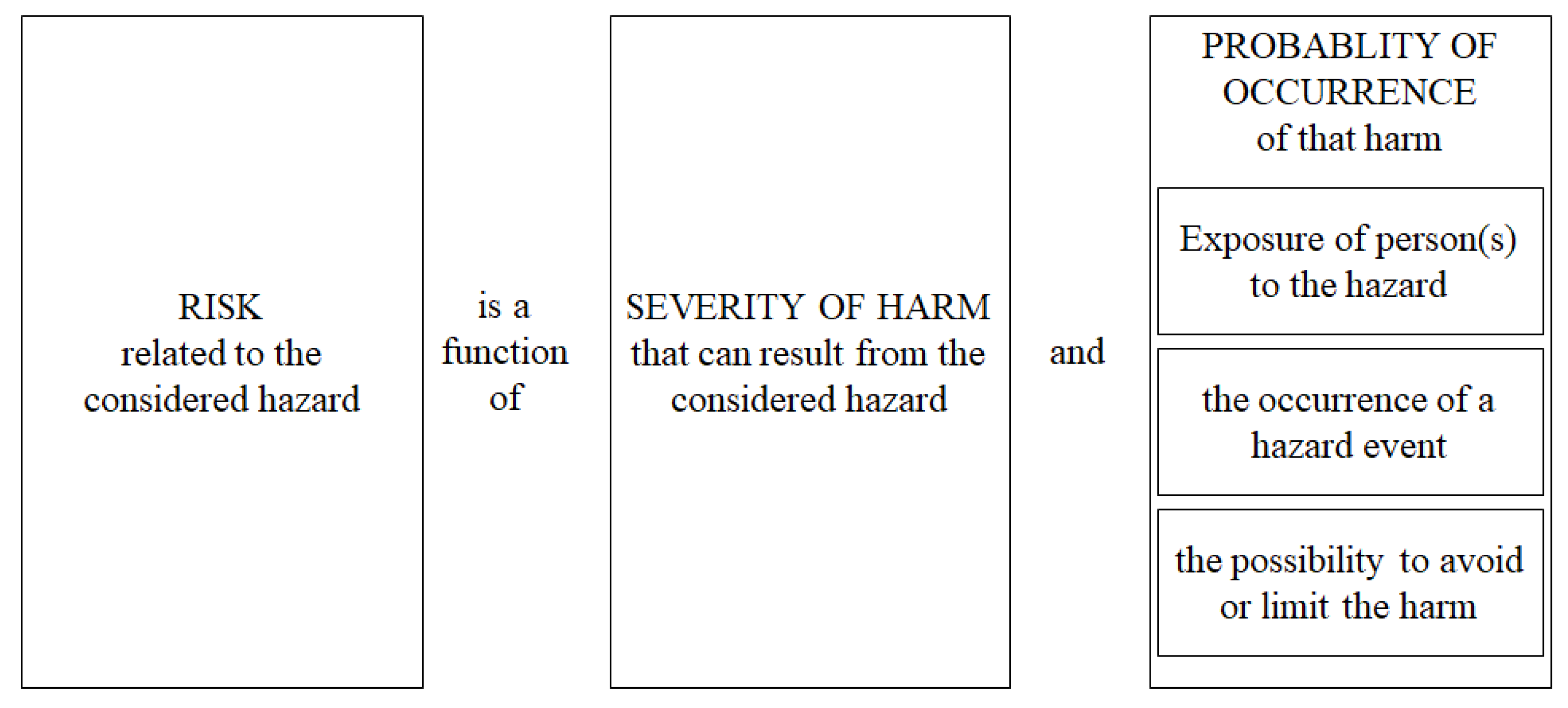
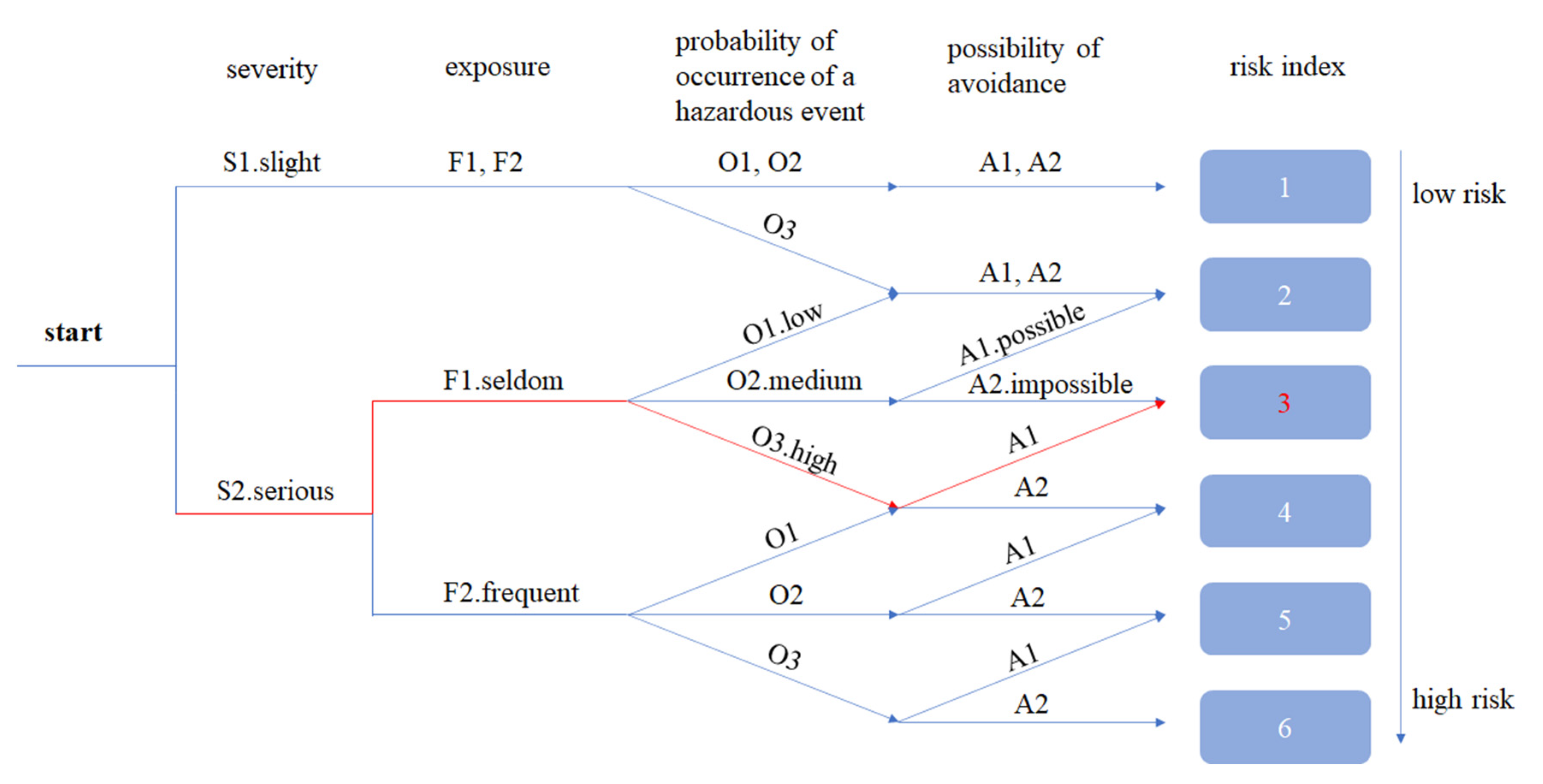
3.2.2. Risk Estimation by Risk Graph Tool

As shown in Figure 3, risk is a function of the severity of harm and the probability of occurrence of that harm, and the probability of occurrence of harm is related to the exposure of person (s) to the hazard, the occurrence of a hazard event, and the possibility to avoid or limit the harm. Each risk element can be divided into discrete scales; the severity of injury S can be divided into two levels, as S1 refers to slight injuries (usually recoverable, e.g., bruises, lacerations, scratches, and other minor injuries requiring first aid), meaning someone cannot perform the same task for less than two days, and S2 refers to serious injuries (usually unrecoverable, e.g., torn or crushed limb, broken bone, serious injury requiring stitches, severe bone injury), meaning someone cannot perform the same task for more than two days. It is customary to employ qualitative (e.g., severe, slight) and quantitative (e.g., two days) words to articulate the distinctions between grades as explicitly and unambiguously as feasible, thereby aiding risk assessors in selecting the most appropriate scale with the utmost accuracy.

The risk estimation tool used to estimate the risk index in this paper was the risk graph method, which is simple and easy to use. In Figure 4, each node represents a risk element in Figure 3, and each branch of the node represents a scale of the risk element. In the risk graph, the path starts from the first branch of severity node; subsequently, it proceeds along the respective branch at each node (exposure, probability of occurrence, and possibility of avoidance) following the selected scale. The final branch points to the risk index of the hazardous situation description, associated with a combination of chosen scales, represented by 1 to 6. For example, if the severity is S2, the exposure is F1, the probability of occurrence of a hazard event is O3, and the probability of avoidance is A1, then the corresponding risk index of this hazard event is 3, as shown by the red arrows in Figure 4.

3.3. The Principle of LSTM-Based Risk Estimation Methodology

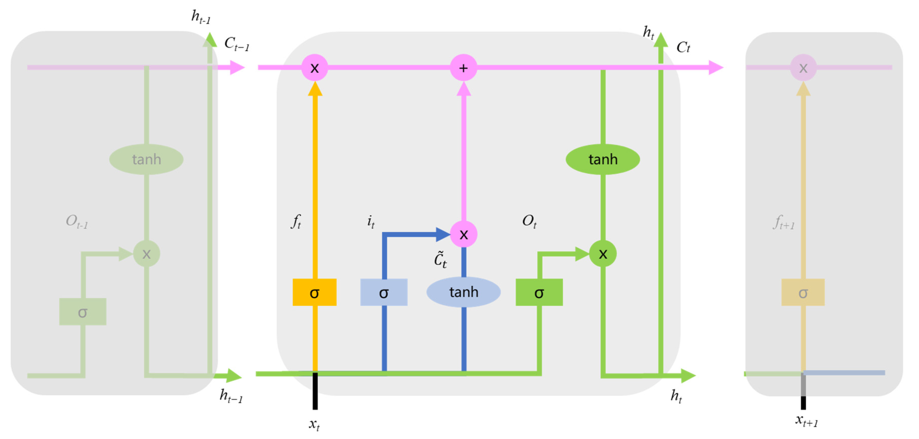
3.3.1. LSTM Algorithm

The LSTM network is a special kind of Recurrent Neural Network (RNN) capable of effectively addressing the problems occurring in traditional RNNs: (1) gradient disappearance/gradient explosion; and (2) long-term dependencies. LSTM has been refined and popularized in many fields, such as time series data processing, text classification, fault prediction, etc. As mentioned in Section 3.2.1, the result of hazard identification can be described by textual descriptions, and the risk index of each hazard situation can be represented by discrete levels. Thus, the risk estimation problem can be converted into a text classification problem.

The core idea behind LSTM network is that its cell state can run straight down the entire chain with some minor linear interactions [28,29], shown by the pink horizontal arrows in Figure 5. Thus, the unaltered transmission of information along this chain is straightforward. An LSTM cell has three gates: the forget gate (orange color in Figure 5), the input gate (blue color in Figure 5), and the output gate (green color in Figure 5); the functions of these three gates are delineated as follows.

The forget gate is used to determine the information to be retained in the cell state (or what information we are going to throw away from the cell state). It is controlled by a sigmoid layer called “forget gate layer”, whose mathematical representation is as shown in Equation (1).

$$f_t=\sigma \left(W_f\cdot \left[h_{t-1},x_t\right]+b_f\right)$$

(1)

The input gate is used to determine what new information we are going to store in the cell state, consisting of two parts: a sigmoid layer called “input layer” is used to determine which values to update, as in Equation (2); and a “tanh” layer is used to create a new vector of candidate values, as in Equation (3).

$$i_t=\sigma \left(W_i\cdot \left[h_{t-1},x_t\right]+b_i\right)$$

(2)

$${\tilde{C}}_t=\tanh \left(W_C\cdot \left[h_{t-1},x_t\right]+b_c\right)$$

(3)

The cell state is updated as in Equation (4): Multiply the old state C_t−1 by 𝑓_𝑡, forgetting what was decided to ignore. Add $i_t*{\tilde{C}}_t$, the new candidate values, scaled by how much it was decided to update each state value.

$$C_t=f_t\ast C_{t-1}+i_t*{\tilde{C}}_t$$

(4)

The output gate has two steps: decide what parts of the cell state we are going to output by a sigmoid layer, put the cell state through “tanh”, and multiply it by the output of the sigmoid gate, as in Equations (5) and (6).

$$O_t=\sigma \left(W_o\cdot \left[h_{t-1},x_t\right]+b_o\right)$$

(5)

$$h_t=o_t\ast \tanh \left(C_t\right)$$

(6)

3.3.2. The LSTM-Based Deep Learning Network Architecture

The LSTM-based deep learning network architecture designed for risk estimation is shown in Figure 6, including six layers: sequeceInputLayer, wordEmbeddingLayer, lstmLayer, fullyConnectedLayer, softmaxLayer, and classificationLayer. The function of each layer is as follows:

sequeceInputLayer: Input the sequences corresponding to the hazardous situation descriptions to the network.

wordEmbeddingLayer: The word-embedding layer maps the sequence of word indices to embedding vectors and learns the word embedding during training. It processes the sequences into word vectors, representing the sequences of corresponding hazardous situation descriptions with low-dimensional dense vectors. The embedding vectors can effectively capture specific attributes of the related objects, and the distance between these vectors serves as an indicator of the similarity between the objects [30].

lstmLayer: The output mode of this layer was set to output the last time step of the sequence, realizing sequence (embedding vectors representing hazardous situation description)-to-label (risk index of the corresponding hazard event) classification [31]. See Section 3.3.1 for the principle of the lstmLayer algorithm.

fullyConnectedLayer: A fully connected layer connects the output of lstmLayer to the risk indices, which multiplies the input by a weight matrix and then adds a bias vector. All neurons in a fully connected layer connect to all those neurons in the previous layer. So, this layer combines all of the features (local information) learned by the previous layers to classify the sequence. In Equation (7), Z denotes the output of the ith node, X_t denotes time step t of X, W denotes weight matrix, and b denotes bias matrix.

$$Z=W{X}_t+b$$

(7)

softmaxLayer: Converts the output of fullyConnectedLayer to the probability corresponding to each risk index. The “softmax” function is applied to the input of the layer, and the output value of the multiclass classification can be transformed into a probability distribution within the specified range [0, 1]. The sum of the probability is 1. Where y is the output value of the ith node, C is the number of output nodes, that is, the number of risk indices for risk estimation, as shown in Equation (8).

$$soft\max \left(y_i\right)=\frac{e^{y_i}}{{\displaystyle \sum _{c=1}^C{e}^{yc}}}$$

(8)

classificationLayer: The classification layer calculates the cross-entropy loss (Equation (9)) for classification tasks with mutually exclusive classes and weighted classification tasks, obtaining the risk index corresponding to the hazardous situation description utilizing sequence-to-label classification. In the classification layer, the training network takes values from the “softmax” function. It assigns each input to one of the K mutually exclusive classes using the cross entropy function for a 1-of-K coding scheme [32].

$$loss=-\frac{1}{N}{\displaystyle \sum _{n=1}^N{\displaystyle \sum _{i=1}^C{w}_i{t}_{ni}\ln y_{ni}}}$$

(9)

where N is the size of the training dataset, C is the number of risk indices, w_i is the weight for risk index i, t_ni is the indicator that the nth hazardous situation belongs to the risk index i, y_ni is the probability that the network associates hazardous situation description n with risk index i, which is the output of softmaxLayer.

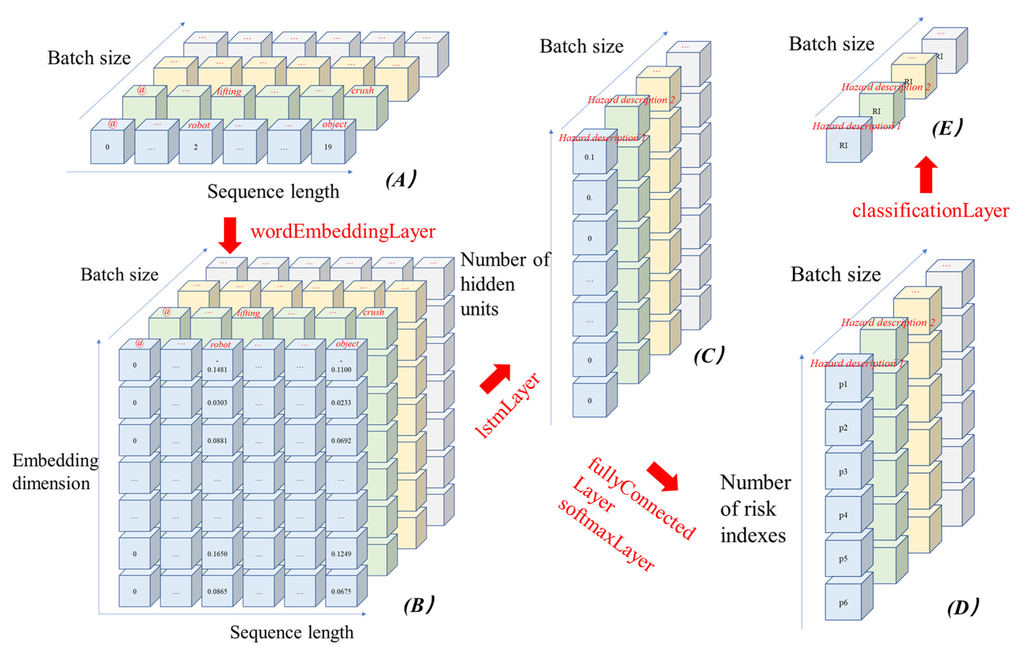
3.3.3. Data Flow across the LSTM-Based Deep Learning Network Layers

To more effectively elucidate the training procedure of the LSTM-based deep learning networks, the data flow for hazardous situation descriptions processed by each network layer is shown in Figure 7. During the training process, a specific number (Batch_size in this paper) of sequences associated with hazard descriptions were extracted from the training dataset each time to create a subset, which is utilized for computing network parameters and updating them only once, a cycle of A-B-C-D-E, as shown in Figure 7. Upon employing all the training data, the average value was used for fine-tuning the entire network’s parameters. For each training subset, the changes in data flow across the network layers are as follows:

(A) The input of wordEmbeddingLayer is a two-dimensional matrix, the size of which is (Batch_size, Sequence_length), wherein Batch_size is the size of training subset, Sequence_length is the length of hazardous situation description. Each row of the two-dimensional matrix represents the sequence of a hazardous situation description.

(B) After passing through the wordEmbeddingLayer, the data are a three-dimensional matrix, the size of which is (Batch_size, Embedding_dimension, Sequence_length). The index of each word in the dictionary is transformed into an embedding vector (the size of the vector is Embedding_dimension) after word-embedding processing. For example, the index of the word “robot” in the dictionary is 2, which is changed into [−0.1481, 0.0303, 0.0881, …, 0.1650, 0.0865] after word embedding.

(C) The data are sequentially input into the lstmLayer according to the length of the Sequence_length step. The data size for each step is (Batch_size, Embedding_dimension, 1), indicating that the data of each step are processed by a LSTM cell unit. Given that the output mode of LSTM is set to “last”, the output data have a size of (Batch_size, Number_hidden_units). Thus, each hazardous situation description will correspond to a vector of size Number_hidden_units, which encapsulates the features of the risk indices.

(D) After being processed by fullyConnectedLayer and softmaxLayer, the data will be transformed into a size of (Batch_size, Number_risk_index, 1). The risk index corresponding to each hazardous situation is a six-element probability vector. Each element of this vector signifies the likelihood of the hazardous situation being associated with one of the six risk indices, 1 to 6, respectively.

(E) After processing by the classificationLayer, the risk index of each hazardous situation description in the training subset is computed.

4. Results

4.1. Test Environment

The development environment chosen for this study was Matlab R2022b, accompanied by Deep Learning Toolbox 14.5, Statistics and Machine Learning Toolbox 12.4, and Text Analytics Toolbox 1.9 [33]. Deep Learning Toolbox is an essential framework for designing and implementing deep neural networks with algorithms, pretrained models, and apps. Users can use convolutional neural networks and long short-term memory networks to perform classification and regression on image, time-series, and text data. The experiment was carried out on the development platform with 12th Gen Intel^®Core™i5-1235U and single GPU NVIDIA GeForce MX550.

4.2. Raw Hazard Event Dataset

The raw hazard event dataset originated from the industrial robot products certification of China Robot Certification(CR) [34] and CE [35]. The related robot products are shown in

Table 1. Related industrial robot products to establish the raw hazard event dataset.

Company Name	Product Name	Product Model
Chengdu CRP Robot Technology Co., Ltd. (Chengdu, China)	Industrial robot	CRP-RH18-20, RRP-RH14-10
KUKA (Foshan, China)	Industrial robot	KR 6 R2010-2 arc HW E, KR 6 R1440-2 arc HW E
Estun Automation (Nanjing, China)	Industrial robot	ER20-1000-SR, ER6-600-SR, ER3-400-SR
STEP (Shanghai, China)	Industrial robot	SR20/1700, SR50/2180, SR165/2580, SR60/2280B

. Risk identification and estimation was conducted by the robot company under the supervision of experts from the certificate authority, following the guidelines provided in [1]. Hazard event descriptions were recorded based on the risk elements outlined in Section 3.2.1, and the tool employed for risk estimation is detailed in Section 3.2.2. The final risk evaluation reports underwent a thorough review by the certificate authority.

The dataset of raw hazard events comprises 93 risk events, and their distribution based on risk indices is presented in

Table 2. Distribution of raw hazard event dataset according to risk index.

Risk Index (RI)	1	2	3	4	5	6
Number of hazardous situation description	9	39	17	17	11	0

. The risk graph method in Section 3.2.2 consists of six levels, but the dataset did not include any hazard event at risk index (RI) = 6.

Figure 8 illustrates the classification and corresponding quantity distribution of the hazard event dataset based on the elements of the hazardous situation descriptions in Figure 2, including phase of life cycle, task, possible states of machine, person, and hazard. The task element, among them, exhibited a high degree of diversity in terms of type, posing challenges in the analysis and quantification process particularly when the number of hazard events was limited. The life cycle involved a total of six stages, cleaning/maintenance, fault-finding/troubleshooting, installation and commissioning, operation, teaching, and transport. Possible states of machine were classified into two categories: normal state, and abnormal state. The use of the machinery by persons included the intended use and reasonably foreseeable misuse/unintended behavior. Hazard types were grouped into mechanical hazards, electrical hazards, thermal hazards, heat, etc.

4.3. Training and Optimization of LSTM-Based Deep Learning Network

4.3.1. Experiment on the Raw Hazard Event Dataset

The text length distribution of hazardous situation descriptions in the dataset is shown in Figure 9, most of which have fewer than 70 tokens (words), which was set as the target length for truncation and padding to facilitate subsequent processing. The input dataset was partitioned, with 80% of the data used as the training set and a held-out proportion (20%) for validation.

The dictionary compiled from the hazardous situation descriptions in the training set comprised 487 words. Utilizing the “wordcloud” function in Matlab Text Analytics Toolbox™, a word cloud diagram can be generated based on the occurrence of words within hazardous situation descriptions, as depicted in Figure 10.

Given the inherent stochasticity of deep learning, variations in outcomes may arise from individual training runs. To accurately assess the efficacy of training, this experiment conducted 30 repetitions of training using the same conditions, and the test results are shown in Figure 11. The comparison revealed that the trained network based on the raw hazard event dataset exhibited a remarkably high accuracy of nearly 100% on the training set; in contrast, its performance on the validation set was relatively subpar, with a median accuracy of only 55.56%, indicating overfitting during the training process and limited generalization ability. To address this issue, the hazard event dataset was augmented to mitigate overfitting effects and enhance model generalization ability, yielding promising results, as demonstrated in Section 4.3.2.

4.3.2. Training and Optimizing the Network Based on the Augmented Hazard Event Dataset

Hazardous situation descriptions belong to textual data. To minimize any alteration in the semantic meaning of risk events, the sentence refinement function of Youdao AIBox (version 10.1.0) [36] was utilized to expand the raw hazard event dataset. The refinement mode of Youdao AIbox encompassed six distinct styles, namely professional, scholarly, colloquial, amiable, more exquisite, and more concise. For each refined statement, Youdao AIbox will give the user the purpose and place of the changes. For example, a hazardous situation description “The robot is lifting in transport phase. operator is placing robot on transportation pallet. operator is crushed between fixed object and robot because of unexpected movement of the robot arm due to slipping breaks.” refined by the professional style is “The robot is being lifted during the transportation phase. The operator is placing the robot onto a transportation pallet. Unfortunately, due to unexpected movement of the robot arm caused by slipping brakes, the operator becomes trapped between a fixed object and the robot”. The refined sentence has been modified in the following aspects: (a) the action description was made more specific, using the continuous tense to express that the robot is being lifted and the operator is placing it on a transport pallet; (b) more formal vocabulary was used, such as “transportation phase” instead of “transportation phase”; and (c) the unexpected movement of the robot arm due to brake slip in an unexpected situation was described.

The experiments on the augmented hazard event dataset were divided into two groups to investigate the influence of text augmentation: (A) the size of the dataset was doubled (2×), and (B) the size of dataset was augmented six times (6×). The corresponding risk index for each hazard event remained unchanged in A and B. As shown in Figure 12, the accuracy rate of the trained network on both 2× and 6× training datasets has reached 100%. The augmentation of the hazard event dataset led to a significant improvement in the accuracy of the trained network on the validation dataset, resulting in a median accuracy increase from 55.56% to 96.92%.

4.3.3. Analysis of Risk Deviation on the Validation Dataset

To further investigate the performance of the trained network on the validation dataset, an analysis of the risk deviation was conducted. Given the LSTM-based deep learning network’s remarkable accuracy and stability on the validation set following training on the 6× augmented dataset, the discussion was based solely on that.

The deviation of the risk estimation RI_deviation was defined as in Equation (10):

$$R{I}_{deviation}=R{I}_P-R{I}_T$$

(10)

RI_p is the predicted value of the risk index by the trained network, and RI_T is the risk index given by the hazard event dataset. Through statistical analysis of risk estimation deviation presented in

Table 3. Risk deviation of the trained network on validation data of 6× augmented dataset.

RIdeviation	−4	−3	−2	−1	1	2	3	4	Total
Quantity	9	7	10	39	18	25	7	3	118
Proportion	7.63%	5.93%	8.47%	33.05%	15.25%	21.19%	5.93%	2.54%	100%

, it was evident that 92 instances exhibited a small deviation, denoted by |RI_deviation| ≤ 2, which accounted for approximately 80% of the total instances. The proportion of instances exhibiting large deviations, defined as |RI_deviation| ≥ 3, was about 20%.

To further investigate the potentially discriminatory of the trained network when there was a deviation in risk estimation, specifically towards overestimation or underestimation of risks, the risk estimation discrimination factor RI_dis is defined as in Equation (11).

$$R{I}_{dis}=\frac{count\left(R{I}_{+}\right)}{count\left(R{I}_{-}\right)}$$

(11)

count (RI₊) represents the number of instances with overestimation, and count (RI₋) represents the number of instances with underestimation. RI_dis = 1 means that the trained network is non-discriminatory, RI_dis << 1 means that the trained network tends to underestimate the risk in the case of risk estimation deviation, RI_dis >> 1 means that the trained network tends to overestimate the risk in the case of risk estimation deviation. The farther away from 1, the more pronounced the tendency is. Through the analysis of the data in Table 3, RI_dis = 0.82, which is close to 1, indicating that the trained network has no obvious bias in risk estimation on the validation dataset when deviation occurs.

4.4. Risk Estimation of New Hazard Events by the Trained Network

To assess the effectiveness of the trained network in handling new hazard events, a subset of hazard events was randomly extracted from the dataset while ensuring no compromise to the efficacy of the training process, and the remaining hazard events were utilized as the dataset for network training. The experiments were divided into two groups: (C) randomly extracting 35 hazard events from the 6× augmented dataset as representative examples for estimating the risk of new hazard events similar to the existing ones in the dataset; and (D) randomly extracting five raw hazard events and their corresponding augmented hazard events (totaling 35 = 5 × 7) as distinct instances for estimating the risk of new hazard events completely different from the existing ones in the dataset.

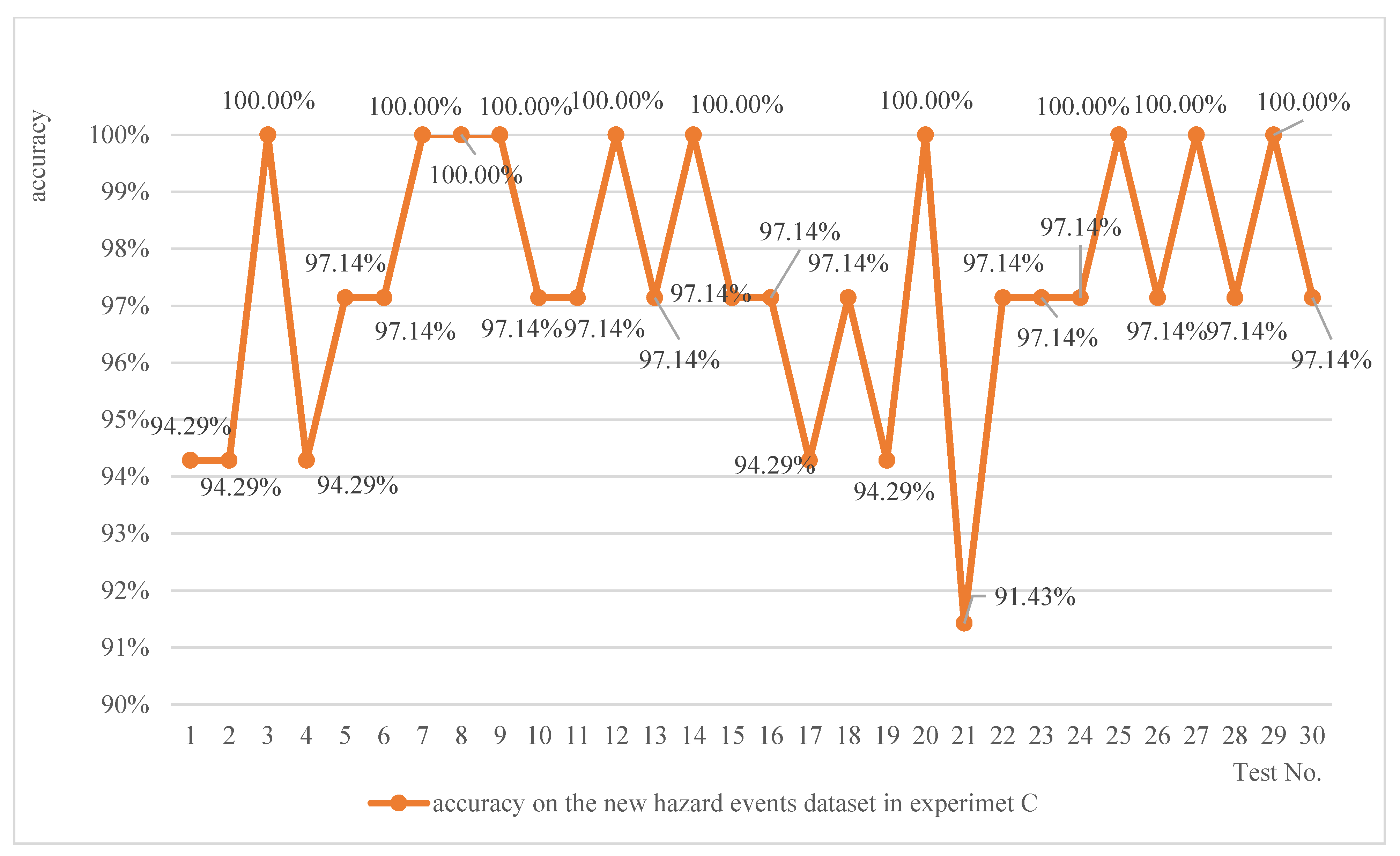
4.4.1. Estimating the Risk of New Hazard Events Similar to the Existing Ones

Experiment C involved 30 repetitions of training runs under the same conditions as those described in Section 4.3. Each test run involved random sampling to create both the new hazard events set and the training set, following rule C, mentioned earlier. The experiment results are shown in Figure 13, where the trained network achieved a maximum accuracy rate of 100% and a minimum of 91.43% for estimating risks associated with the new hazard events, with a median value of 97.14%, and the standard deviation of the thirty test runs was 0.023, indicating that the trained network exhibits robust stability in estimating risks associated with new hazard events similar to the existing ones.

Approximately 85.18% of the deviation instances in experiment C were classified as small deviations. In comparison, less than 20% were large deviations. According to Equation (11), the risk estimation discrimination factor RI_dis was 0.93, which was close to 1, indicating no discernible bias in the trained network to estimate the risk of new hazard events similar to the existing ones.

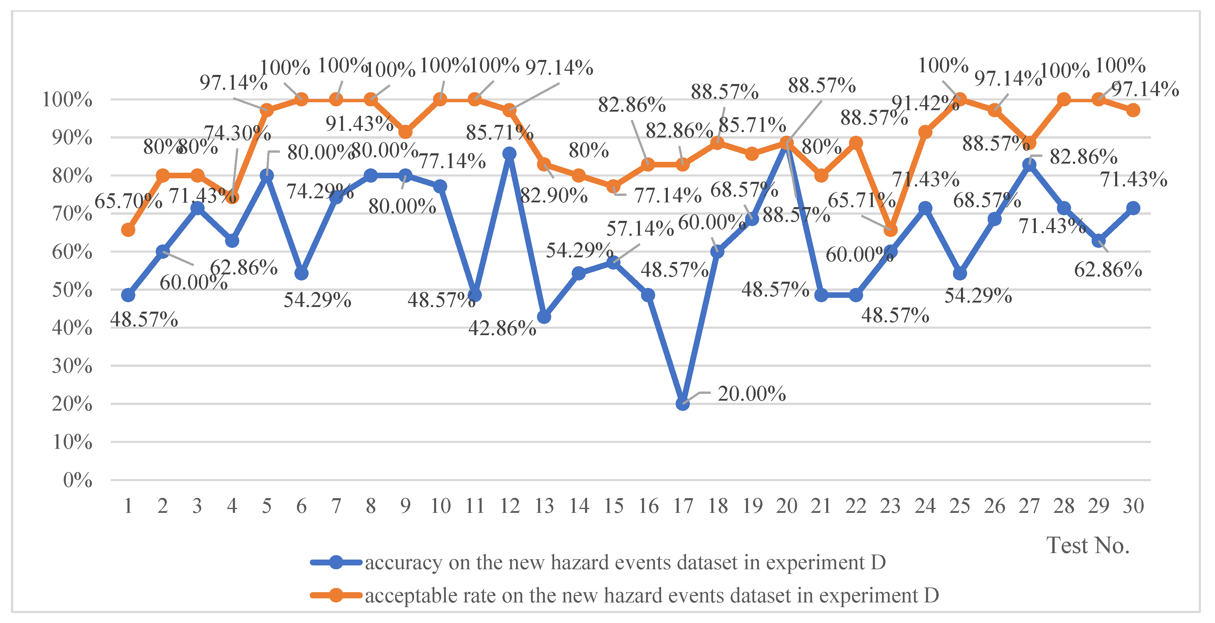
4.4.2. Estimating the Risk of New Hazard Events Completely Different from the Existing Ones

Experiment D involved 30 repetitions of training runs under the same conditions as those described in Section 4.3. Each test run involved random sampling to create both the new hazard events set and the training set, following rule D, mentioned above. The experiment results are shown in Figure 14, where the trained network achieved a maximum accuracy rate of 88.57% and a minimum of 20.00% for estimating risks associated with these new hazard events, with a median value of 62.86%, and the standard deviation of the thirty test runs was 0.149.

The trained network in experiment D also showed a high likelihood of small deviation in the case of risk estimation deviation, with 88.67% of the instances classified as small deviations. According to Equation (11), the risk estimation discrimination factor RI_dis was found to be 1.23, which was close to 1. Regarding the new hazard event dataset, which was completely different from the existing ones, if a small deviation of risk estimation was acceptable, the acceptable rate is depicted as the orange dashed line Figure 14. The maximum acceptable rate for estimating risks associated with new hazard events was 100.00%, with the median value determined to be 88.57%. Therefore, the experimental results lead to a conclusion that the trained network shows trustworthiness in estimating the risk of hazard events completely different from the existing ones.

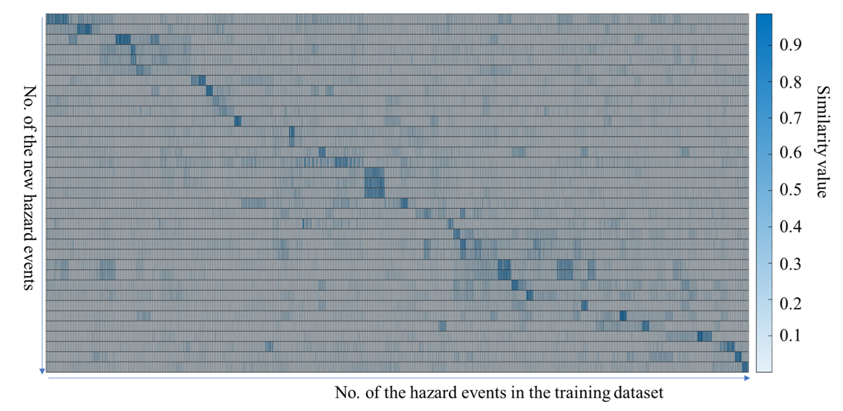
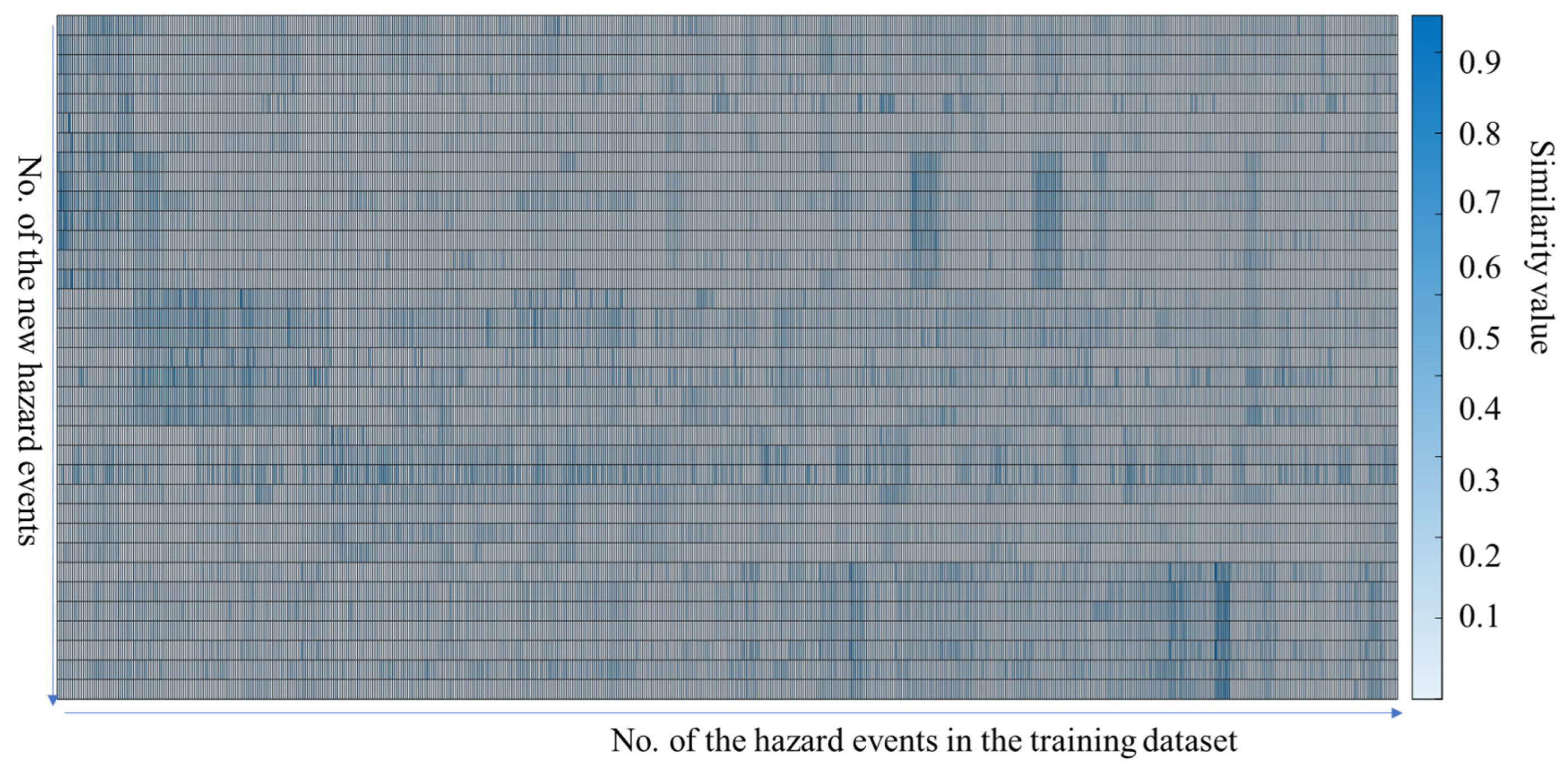
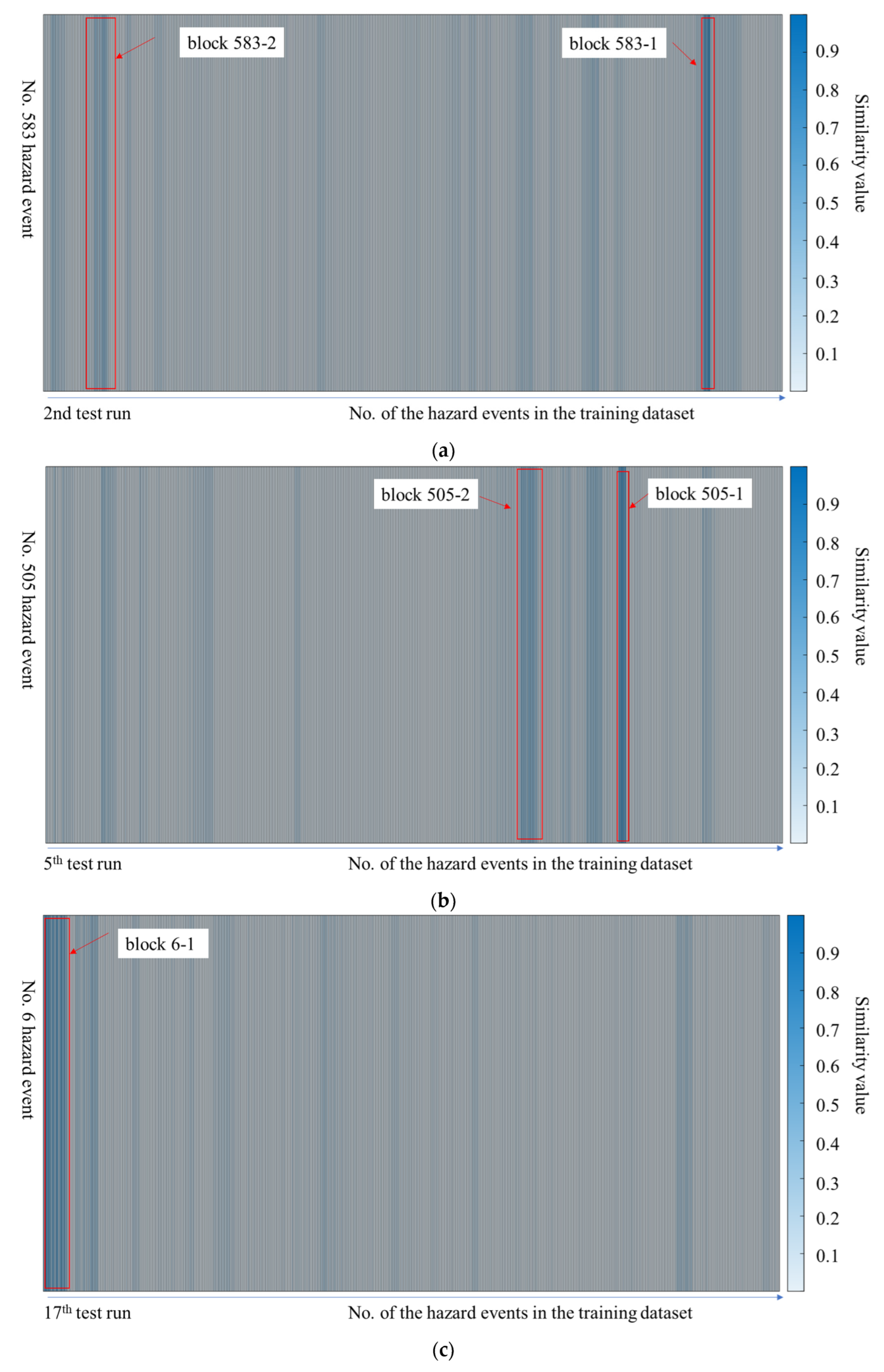
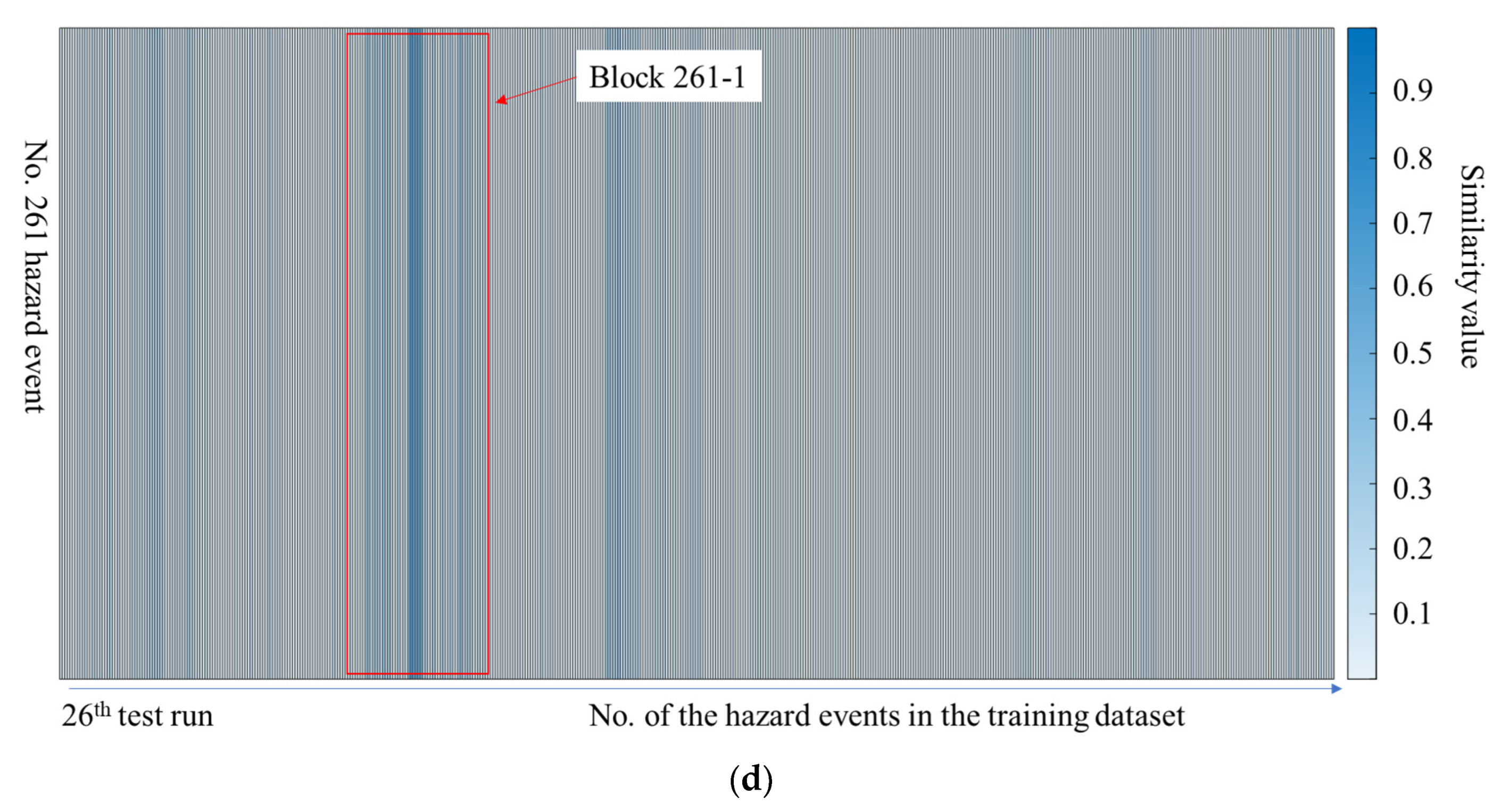
4.4.3. The Similarity between the New Hazard Events and the Existing Ones

As indicated in Section 4.4.1, the trained network demonstrated robust stability in estimating risks associated with new hazard events similar to the existing ones. However, it was observed that for certain dissimilar hazard events, as discussed in Section 4.4.2, there were large deviations observed in risk estimation with a specific probability. Therefore, assessing the degree of similarity between a new hazard event and existing ones is crucial for effectively utilizing the LSTM-based risk estimation methods. In this paper, similarities between the new hazard events and the ones in the training dataset were investigated by the cosine similarity method, a mathematical method using the similarity between texts as in Equation (12), derived from the calculus of vectors in mathematics [37].

$$\cos \left(\theta \right)=\frac{{\displaystyle \sum \left(a_i{b}_i\right)}}{\sqrt{a_i^2}\sqrt{b_i^2}}$$

(12)

where a_i and b_i represent the vector values of the two texts (hazardous situation descriptions), respectively. Scores close to one indicate strong similarity; scores close to zero indicate a weak similarity.

The heat map in Figure 15 illustrates the similarities between the new hazard events and the training dataset in the first test run of experiment C, while Figure 16 presents the similarities between the new hazard events and the training dataset in the first test run of experiment D. The horizontal axis in the heatmap represents the number of hazard events in the training dataset, with augmented hazard events originating from the same source positioned adjacent to each other. The vertical axis represents the number of the new hazard events, and the color depth represents the similarity between the new hazard event and the No.i (1 ≤ i ≤ 651) hazard event in the training dataset. Comparing these two figures, it is evident that in experiment C, the new hazard events can readily identify their similar ones—represented by dark-clustered color blocks. Conversely, in experiment D, the new hazard events face difficulty in doing so. Based on the results of experiment C, it can be inferred that the risk index of new hazard events primarily depends on the risk index of highly similar hazard events in the training dataset.

In experiment C, No.583 hazard event in the 2nd test run, No.505 hazard event in the 5th test run, No.6 hazard event in 1the 7th test run and No.261 hazard event in the 26th test run were large deviations. Similarities between these new hazard events and their corresponding training dataset are shown in Figure 17. There were two dark-clustered blocks in Figure 17a,b, while there was a single wide dark-sparse block in Figure 17c,d, which implied that multiple existing hazard events in the training dataset exhibited similarities to the new hazard event.

The details of the blocks in Figure 17a were enumerated in

Table 4. Details of blocks in Figure 17a.

New Hazard Events’ Risk Estimation Deviation			Block No.	Similar Hazard Events in the Training Dataset			The Same Raw Hazard Event
No.	True Risk Index	Estimated Risk Index		No.	Similarity Value	Risk Index
583	5	2	583-1	584	0.7423	5	Yes
				585	0.459	5	Yes
				586	0.5761	5	Yes
				587	0.6821	5	Yes
				588	0.7426	5	Yes
			583-2	50	0.2477	2	No
				51	0.3278	2	No
				53	0.2304	2	No
				54	0.2269	2	No
				55	0.1647	2	No
				56	0.2155	2	No
				57	0.2796	2	No
				58	0.346	2	No
				59	0.3889	2	No
				60	0.2923	2	No
				61	0.2947	2	No

to conduct a more comprehensive investigation into the underlying causes of risk estimation deviation. The true risk index of No.583 was RI 5, but the estimated risk index by the trained network was RI 2. Although No.583 had a high similarity to No.584~No.588, which originated from the same raw hazard event with a risk index of 5, it also demonstrated certain similarities to No.50~No.61, originating from different raw hazard events with a risk index of 2. Therefore, in cases where multiple events with low similarity to the new hazard event are present in the training set, their cumulative impact may surpass or equal that of high similarity events, leading to a deviation in risk estimation. The deviations observed in experiment D were also examined using the cosine similarity method, yielding the same conclusion as that of experiment C.

4.5. Comparison with Other Methods

The risk estimation problem was transformed into a text classification task using LSTM-based deep learning methods, as discussed in Section 3.3.1. Therefore, it is plausible to explore the utilization of other natural language-processing techniques for conducting risk estimation. The present study investigates the utilization of convolutional neural networks (CNN) [38] and bidirectional long short-term memory (bi-LSTM) [39] networks, in comparison with an LSTM-based risk estimation method, for estimating the risk associated with the new hazard events completely different from the existing ones. The experimental findings are presented in

Table 5. Comparison of the three methods.

Risk Estimation Method	Accuracy			Acceptable Rate			Percentage of Small Deviation	RIdis
	Min	Median	Max	Min	Median	Max
bi-LSTM-based	5.71%	58.57%	80.00%	60.00%	94.29%	100.00%	90.29%	1.25
LSTM-based	20.00%	62.86%	88.57%	65.70%	88.57%	100.00%	88.76%	1.23
CNN-based	40.00%	70.00%	94.29%	65.71%	97.14%	100.00%	91.62%	0.51

.

The comparison results indicate that in terms of median accuracy, the CNN-based approach outperforms both LSTM-based and bi-LSTM-based approaches. Regarding the median acceptable rate, the CNN-based approach surpasses the bi-LSTM-based and LSTM-based approaches. Furthermore, for ensuring stable risk estimation, the CNN-based approach demonstrates superiority over both LSTM-based and bi-LSTM-based approaches. The percentages of small deviation exhibited similar values across the three methods.

Although the CNN-based method achieved a relative higher accuracy and acceptable rate, RI_dis = 0.51, it tends to underestimate the risk of the hazard event when deviations occur, which is undesirable in risk estimation. Among the three methods, the LSTM-based risk estimation method demonstrates no significant bias when deviations occur, effectively balancing accuracy and stability in risk estimation.

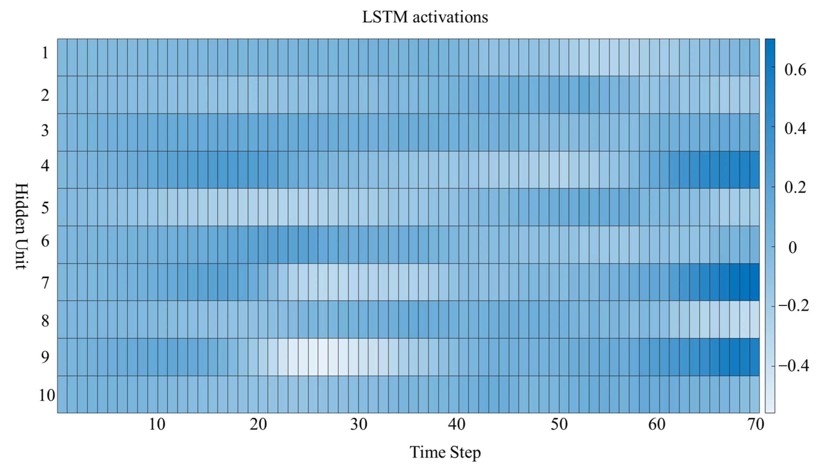
4.6. Model Explanation

Deep learning networks are often described as “black boxes” because the reason that a network makes a certain decision is not always obvious. Interpretability techniques are used to translate network behavior into output that a person can interpret, such as locally interpretable model-agnostic explanations (LIME) [40], a Shapley value [41], and visualization methods. To explore the activations of the LSTM-based risk estimation method, activations were extracted to investigate and visualize the features learned by the LSTM network. Figure 18 shows the activations output by the LSTM layer (third layer) for each time step of the sequences in estimating the risk index of the hazard event—“The robot is being lifted during the transportation phase, while the operator carefully positions it onto a transportation pallet. The operator remains in close proximity to the robot throughout the lifting process. Unfortunately, due to an unstable lift, the operator becomes trapped between a fixed object and the robot”. The heatmap showed how strongly the first 10 hidden units (a total of 250) activated and highlighted how the activations changed over time (the sequence length).

5. Discussion

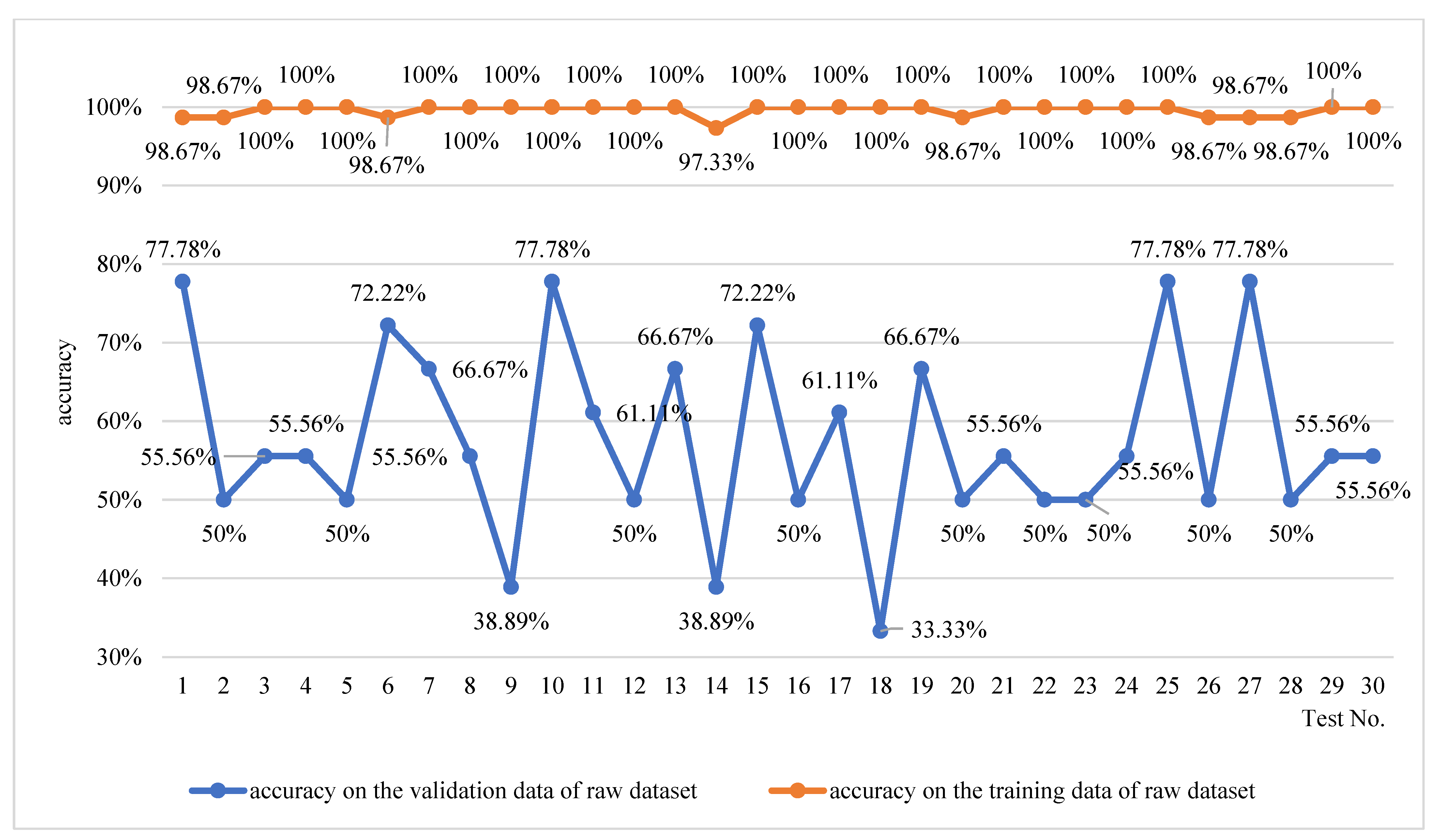
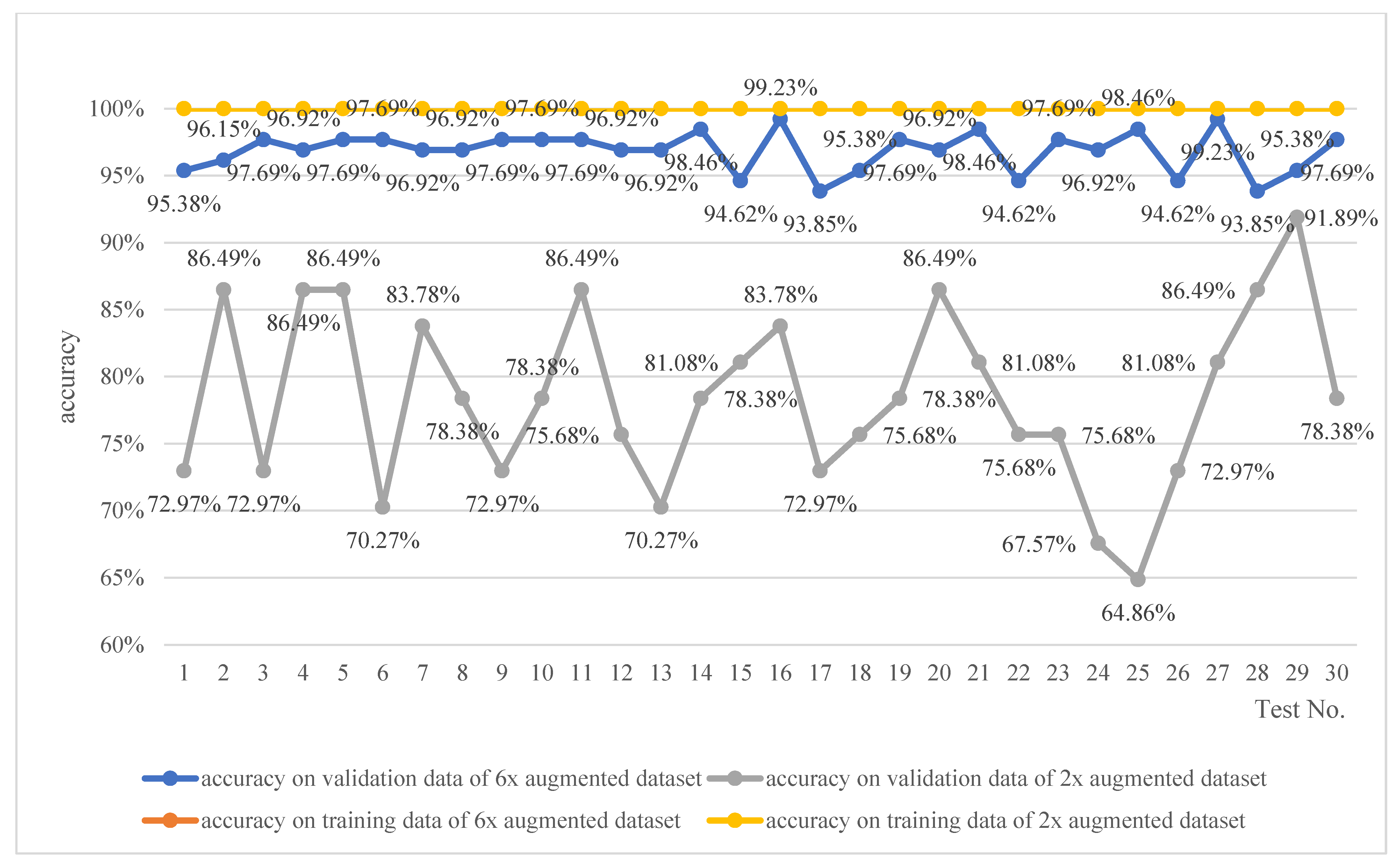
• In the raw hazard event dataset experiment, the overfitting problem aroused due to the limited dataset. Comparing the performance of the trained network based on the raw dataset, 2× augmented dataset, and 6× augmented dataset, as shown in

  Table 6. Comparison of the trained network based on the raw dataset and augmented dataset.

  Accuracy	Training Dataset			Validation Dataset
  	Max	Min	Median	Max	Min	Median	Standard Deviation
  raw dataset	100%	97.33%	98.67%	77.78%	33.33%	55.56%	0.118
  2×	100%	100%	100%	91.89%	64.86%	78.38%	0.065
  6×	100%	100%	100%	99.23%	93.85%	96.92%	0.015

  , the augmentation of the hazard event dataset led to a significant improvement in the accuracy and reduction in the standard deviation on the validation dataset.

2.

The trained network exhibits robust stability in estimating risks associated with new hazard events similar to the existing ones in the training dataset, achieving a maximum accuracy rate of 100% and a minimum of 91.43%, with a median value of 97.14%. Considering that an acceptable rate should ideally reach up to 100%, with a median value of 88.57%, the trained network demonstrates trustworthiness in estimating the risk of hazard events complexly different from the existing ones.

3.

It is found that nearly 80% were small deviations (|RI_deviation| ≤ 2) and the discrimination factor RI_dis is close to 1. That means the proposed method has a high likelihood of reaching a smaller deviation in the case of risk estimation deviation with no obvious bias, which proves the effectiveness of the proposed method in risk estimation.

4.

Among the CNN-based, bi-LSTM-based and LSTM-based risk estimation methods, the LSTM-based one demonstrates no significant bias when deviations occur, effectively balancing accuracy and stability in risk estimation of new hazard events completely different from the existing ones.

6. Conclusions

Risk estimation is commonly conducted by integrating quantitative and qualitative evaluation of risk assessment group members, which may be influenced by subjective factors introduced by individuals involved in the process, leading to disagreements regarding risk estimation results and hindering a collaborative implementation of more effective risk reduction measures among all safety-related parties.

The LSTM-based risk estimation method was proposed to integrate historical risk estimation data, solidify expert experience, and refine judgments based on the comprehensive analysis of historical products or applications. To facilitate the establishment of a comprehensive dataset of hazard events, the essential elements of hazardous situation descriptions was systematically categorized.

A hazard event dataset of industrial robot originated from CR and CE certification was used to verify the proposed methodology. The experiment demonstrated a substantial improvement in both the accuracy and stability with the augmentation of hazard event dataset. On the new dataset, the trained network also showed near-perfect performance on similar hazard events and trustworthiness on completely different ones. In cases of risk deviations, most of them were small deviation without a noticeable bias.

Risk estimation was “black-boxed” and “digitized” by the LSTM-based deep learning method. Risk group members only need to focus on identifying hazard events, without individual interpretation on the descriptions and grade definitions, or making subjective judgments and choices. Therefore, this approach effectively mitigates the influence of human factors during the risk estimation process. In addition, the historical risk estimation information can be transformed into a digital model, thereby establishing a standardized reference for subsequent risk estimation endeavors in similar domains. This facilitates the development of a unified benchmark for risk assessment within project teams, enterprises, and relevant stakeholders, fostering coordination among parties and promoting the implementation of coordinated security measures.

In terms of implementation, several suggestions are proposed. The training of the network is heavily dependent on the availability and quality of historical risk information. It is advisable to create a high-quality hazard event dataset that specifically pertains to a particular product type or application field. Moreover, similarity analysis between the new event and the training dataset holds significant importance in identifying potential deviations in risk estimation. In cases where there are errors in text similarity matching or multiple matches of equal magnitude, an intervention by risk assessors becomes necessary.

Limitations: The accuracy of the LSTM-based risk estimation method for new hazard events, which are completely different from existing ones, can be enhanced in future studies by incorporating novel deep learning algorithms and employing model explanation techniques. Due to the limitations in laboratory software and hardware resources, the utilization of large-scale models for optimizing risk estimation methods has yielded suboptimal results, exemplified by the Bidirectional Encoder Representations from Transformer (BERT) model at the same test environment and experiment parameters. Even so, considering diverse domains, such as ChatGPT, there is potential for advancing artificial intelligence models to achieve precise risk assessment within specific fields.

References

1. ISO:12100; Safety of Machinery—General Principles for Design—Risk Assessment and Risk Reduction. International Organization for Standardization: Geneva, Switerland, 2010.
2. European Union. Directive 2006/42/EC of the European Parliament and of the Council of 17 May 2006 on machinery, and amending Directive 95/16/EC (Recast) (Text with EEA Relevance). Available online: https://eur-lex.europa.eu/legal-content/EN/TXT/?uri=CELEX:32006L0042 (accessed on 29 October 2023).
3. ISO10218-1:2011; Robots and Robotic Devices—Safety Requirements for Industrial Robots—Part 1: Robots. ISO: Geneva, Switerland, 2011.
4. ISO/TS:15066; Robots and Robotic Devices Collaborative Robots. International Organization for Standardization: Geneva, Switerland, 2016.
5. ISO10218-2:2011; Robots and Robotic Devices—Safety Requirements for Industrial Robots—Part 2: Robot Systems and Integration. ISO: Geneva, Switerland, 2011.
6. ISO13482:2014; Robots and Robotic Devices—Safety Requirements for Personal Care Robots. ISO: Geneva, Switerland, 2014.
7. ISO3691-4:2020; Industrial Trucks—Safety Requirements and Verification—Part 4: Driverless Industrial Trucks and Their Systems. ISO: Geneva, Switerland, 2020.
8. Hietikko, M.; Malm, T.; Alanen, J. Risk estimation studies in the context of a machine control function. Reliab. Eng. Syst. Saf. 2011, 96, 767–774. [Google Scholar] [CrossRef]
9. ISO13849-1:2015; Safety of Machinery—Safety-Related Parts of Control Systems—Part 1: General Principles for Design. ISO: Geneva, Switerland, 2015.
10. ISO61508-5:2010; Functional Safety of Electrical/Electronic/Programmable Electronic Safety-Related Systems—Part 5: Examples of Methods for the Determination of Safety Integrity Levels. ISO: Geneva, Switerland, 2010.
11. ISO14121-2:2012; Safety of Machinery—Risk Assessment—Part 2: Practical Guidance and Examples of Methods. ISO: Geneva, Switerland, 2013.
12. Jocelyn, S.; Ouali, M.-S.; Chinniah, Y. Estimation of probability of harm in safety of machinery using an investigation systemic approach and Logical Analysis of Data. Saf. Sci. 2018, 105, 32–45. [Google Scholar] [CrossRef]
13. Duijm, N.J. Recommendations on the use and design of risk matrices. Saf. Sci. 2015, 76, 21–31. [Google Scholar] [CrossRef]
14. Hubbard, D.; Evans, D. Problems with scoring methods and ordinal scales in risk assessment. IBM J. Res. Dev. 2010, 54, 2:1–2:10. [Google Scholar] [CrossRef]
15. Cox, A.L., Jr. What’s Wrong with Risk Matrices. Risk Anal. 2008, 28, 497–512. [Google Scholar] [CrossRef] [PubMed]
16. Azadeh-Fard, N.; Schuh, A.; Rashedi, E.; Camelio, J.A. Risk assessment of occupational injuries using Accident Severity Grade. Saf. Sci. 2015, 76, 160–167. [Google Scholar] [CrossRef]
17. van Duijne, F.H.; van Aken, D.; Schouten, E.G. Considerations in developing complete and quantified methods for risk assessment. Saf. Sci. 2008, 46, 245–254. [Google Scholar] [CrossRef]
18. Moatari-Kazerouni, A.; Chinniah, Y.; Agard, B. A proposed occupational health and safety risk estimation tool for manufacturing systems. Int. J. Prod. Res. 2015, 53, 4459–4475. [Google Scholar] [CrossRef]
19. Cosgriff, C.V.; Celi, L.A. Deep learning for risk assessment: All about automatic feature extraction. Br. J. Anaesth. 2020, 124, 131. [Google Scholar] [CrossRef] [PubMed]
20. Paltrinieri, N.; Comfort, L.; Reniers, G. Learning about risk: Machine learning for risk assessment. Saf. Sci. 2019, 118, 475–486. [Google Scholar] [CrossRef]
21. Brito, M.P.; Stevenson, M.; Bravo, C. Subjective machines: Probabilistic risk assessment based on deep learning of soft information. Risk Anal. 2023, 43, 516–529. [Google Scholar] [CrossRef] [PubMed]
22. Jocelyn, S.; Chinniah, Y.; Ouali, M.-S. Contribution of dynamic experience feedback to the quantitative estimation of risks for preventing accidents: A proposed methodology for machinery safety. Saf. Sci. 2016, 88, 64–75. [Google Scholar] [CrossRef]
23. Allouch, A.; Koubaa, A.; Khalgui, M.; Abbes, T. Qualitative and Quantitative Risk Analysis and Safety Assessment of Unmanned Aerial Vehicles Missions Over the Internet. IEEE Access 2019, 7, 53392–53410. [Google Scholar] [CrossRef]
24. Zarei, E.; Khakzad, N.; Cozzani, V.; Reniers, G. Safety analysis of process systems using Fuzzy Bayesian Network (FBN). J. Loss Prev. Process Ind. 2019, 57, 7–16. [Google Scholar] [CrossRef]
25. Ruge, B. Risk Matrix as Tool for Risk Assessment in the Chemical Process Industries. In Proceedings of the Probabilistic Safety Assessment and Management, Berlin, Germany, 14–18 June 2004; pp. 2693–2698. [Google Scholar]
26. Hochreiter, S.; Schmidhuber, J. Long Short-Term Memory. Neural Comput. 1997, 9, 1735–1780. [Google Scholar] [CrossRef] [PubMed]
27. ISO/TR22100-1:2021; Safety of Machinery—Relationship with ISO 12100—Part 1: How ISO 12100 Relates to Type-B and Type-C Standards. ISO: Geneva, Switerland, 2015.
28. Colah. Understanding LSTM Networks. Available online: http://colah.github.io/posts/2015-08-Understanding-LSTMs/ (accessed on 7 August 2022).
29. Staudemeyer, R.C.; Morris, E.R. Understanding LSTM—A tutorial into Long Short-Term Memory Recurrent Neural Networks. arXiv, 2019; arXiv:1909.09586. [Google Scholar] [CrossRef]
30. Rong, X. word2vec Parameter Learning Explained. arXiv 2016, arXiv:1411.2738. [Google Scholar] [CrossRef]
31. Kudo, M.; Toyama, J.; Shimbo, M. Multidimensional curve classification using passing-through regions. Pattern Recogn. Lett. 1999, 20, 1103–1111. [Google Scholar] [CrossRef]
32. Bishop, C.M. Pattern Recognition and Machine Learning; Springer: New York, NY, USA, 2006. [Google Scholar]
33. The MathWorks, Inc. Deep Learning Toolbox—Design, Train, and Analyze Deep Learning Networks. Available online: https://www.mathworks.com/products/deep-learning.html (accessed on 15 October 2022).
34. TCAR. Introduction of China Robot Certification. Available online: http://china-tcar.com/Service/Detail?Id=202012301205527916626b3174615cb (accessed on 8 November 2023).
35. European-Commission. CE Marking. Available online: https://single-market-economy.ec.europa.eu/single-market/ce-marking_en (accessed on 8 November 2022).
36. Netease. Youdao AIBox. Available online: https://fanyi.youdao.com/download-Windows?keyfrom=baidu_pc&bd_vid=11741871806532036510 (accessed on 11 November 2023).
37. AlShammari, A.F. Implementation of Text Similarity using Cosine Similarity Method in Python. Int. J. Comput. Appl. 2023, 185, 11–14. [Google Scholar] [CrossRef]
38. Hughes, M.; Li, I.; Kotoulas, S.; Suzumura, T. Medical Text Classification Using Convolutional Neural Networks. Stud. Health Technol. Inf. 2017, 235, 246. [Google Scholar] [CrossRef]
39. Peters, M.E.; Neumann, M.; Iyyer, M.; Gardner, M.; Clark, C.; Lee, K.; Zettlemoyer, L. Deep Contextualized Word Representations. arXiv 2018, arXiv:1802.05365. [Google Scholar]
40. Ribeiro, M.T.; Singh, S.; Guestrin, C. “Why Should I Trust You?”: Explaining the Predictions of Any Classifier. In Proceedings of the International Conference on Knowledge Discovery and Data Mining, San Francisco, CA, USA, 13–17 August 2016; pp. 1135–1144. [Google Scholar]
41. Lundberg, S.; Lee, S.-I. A Unified Approach to Interpreting Model Predictions. arXiv, 2017; arXiv:1705.07874. [Google Scholar] [CrossRef]
Figure 1. Flow chart of LSTM-based risk estimation methodology.
Applsci 14 04519 g001
Figure 2. Critical elements of hazardous situation description.
Applsci 14 04519 g002
Figure 3. Elements of risk.
Applsci 14 04519 g003
Figure 4. Risk estimation using risk graph tool.
Applsci 14 04519 g004
Figure 5. LSTM cell.
Applsci 14 04519 g005
Figure 6. Architecture of LSTM-based deep learning network for risk estimation.
Applsci 14 04519 g006
Figure 7. Sketch of data flow across the LSTM-based deep learning network layers.
Applsci 14 04519 g007
Figure 8. Hazard events classified by elements of hazardous situation descriptions.
Applsci 14 04519 g008
Figure 9. Text length distribution of the raw hazard event dataset.
Applsci 14 04519 g009
Figure 10. Word cloud generated based the training data of raw dataset.
Applsci 14 04519 g010
Figure 11. Results of training the network based on the raw hazard event dataset.
Applsci 14 04519 g011
Figure 12. Results of training the network based on the augmented hazard event dataset.
Applsci 14 04519 g012
Figure 13. Results of risk estimation on the new hazard events in experiment C.
Applsci 14 04519 g013
Figure 14. Results of risk estimation on the new hazard events in experiment D.
Applsci 14 04519 g014
Figure 15. Heatmap of similarities between the new hazard event dataset and the training dataset in the first test run of experiment C.
Applsci 14 04519 g015
Figure 16. Heatmap of similarities between the new hazard event dataset and the training dataset in the first test run of experiment D.
Applsci 14 04519 g016
Figure 17. Heatmap of similarities between the hazard events’ large deviation and the training dataset in experiment C.
Applsci 14 04519 g017aApplsci 14 04519 g017b
Figure 18. Heatmap of the activations output by the LSTM layer for each time step of the sequences in estimating the risk index of new hazard event.
Applsci 14 04519 g018