A New Approach to Detect Hand-Drawn Dashed Lines in Engineering Sketches

Featured Application

This work examines the detection of dashed lines in engineering sketches, a subproblem of the more ambitious challenge of automating the reconstruction of 3D models from sketches (sketch-based modeling), which remains unresolved. The detection of dashed lines helps gather valuable information for the interpretation of sketches and consequently improves the quality of the reconstructed 3D models. Sketch-based modeling remains relevant partly because it is aligned with advances in additive manufacturing, e.g., 3D printing, and the mass customization of manufacturing systems. Sketch-based modeling simplifies the CAD/CAM process and allows non-expert users to create their own designs. It also allows designers to quickly create conceptual prototypes of products from sketches, which facilitates the exploration of ideas.

Abstract

Sketched drawings sometimes include non-solid lines drawn as sets of consecutive strokes. They represent dashed lines, which are useful for various purposes. Recognizing such dashed lines while parsing drawings is reasonably straightforward if they are outlined with a ruler and compass but becomes challenging when they are hand-drawn. The problem is manageable if the strokes are drawn consecutively so we can leverage the entire sequence. However, it becomes more challenging if they are drawn unordered, and/or we do not have access to the sequence (like in batch vectorization). In this paper, we describe a new approach to identify groups of strokes as depicting single hand-drawn dashed lines. The approach does not use sequence information and is tolerant with irregularities and imprecisions of the strokes. Our goal is to identify hidden lines of sketched engineering line-drawings, which would enable the interpretation of line-drawings with hidden edges, which currently cannot be efficiently vectorized. We speculate that other fields like hand-drawn graph interpretation may also benefit from our approach.

1. Introduction

Non-solid lines (also known as discontinuous lines) are commonly used as variants of continuous lines to link a graphical attribute to the lines (a sort of tag associated with the line) as a way to assign specific meaning that is commonly defined in advance and explained in a sort of legend. For instance, a graph displays the mutual relationships between the components of a set of objects. The objects are represented by simple figures (like circles or rectangles, perhaps enclosing textual annotations), which are called vertices. Lines that connect vertices represent relationships between objects. Using lines other than solid ones helps to visualize different types of relationships between the same set of objects (as illustrated in Figure 1).

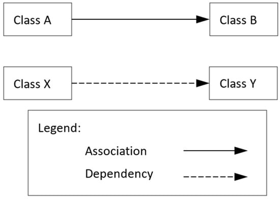
Figure 1. An example diagram illustrating the use of dashed lines to represent relationships between classes in computer code.

In this paper, we describe a new approach to identify hand-drawn dashed lines. Although the approach is intended to be as generic as possible, we are mainly interested in dashed lines used in line-drawings. In this regard, there are typically two types of line-drawings of solid shapes: natural and wireframe. Neither of them includes dashed lines. However, there is also a hybrid type of line-drawings: wireframes with hidden edges represented as dashed lines. This type of drawing is supported by drawing standards (such as ISO 128-2:2020 [1]) and has been—and continues to be—widely used in engineering drawings. It has been historically less common in sketch-based modeling (SBM) because it requires an additional workload from the part of the designer, and it is more challenging for the computer.

In this context, an algorithm that could detect hand-drawn dashed lines would enable SBM approaches to process line-drawings that include hidden edges represented as dashed lines. Such an algorithm would obviously provide information about the type of the edge (visible or hidden) represented by each line, thus easing the procedure to find the 3D shape depicted by the 2D line-drawing. The grouped line would be marked as “dashed”, facilitating the subsequent detection of hidden edges. In addition, such an algorithm would also facilitate the vectorization process by grouping non-solid strokes before they may be—incorrectly—parsed as independent edges. To sum up, an algorithm to detect dashed lines eases vectorization, while providing high-level semantic information that may improve the subsequent reconstruction process.

After justifying the benefits of an algorithm to detect hand-drawn dashed lines, the rest of the paper is organized as follows: We first review the related work to conclude that—to the best of our knowledge—no similar algorithms have been published so far. The problems the algorithm could solve are faced by alternative approaches that require human intervention and/or limit the scope of the automatic approaches. In Section 3, we describe the general process of vectorization to provide context and understanding of the objective and tasks of the algorithm under consideration in this work. In Section 4, we detail the main guidelines of our approach. In short, we assume that short strokes are candidate dashes, and then we recursively find chains of such candidate dashes by searching for dashes that precede or follow the current chain until no more candidates remain and/or they do not meet the requirements. We use a set of geometric and perceptual criteria to guide the search for the most plausible dashes. The tuning parameters that govern those criteria are first introduced in Section 4 and summarized in Section 5. A collection of varied examples is used to validate the approach and evaluate its goodness in Section 6. Finally, the concluding remarks are outlined in the last section.

2. Related Work

The problem of reconstructing 3D shapes from 2D drawings is challenging, as the information provided by the user is a flat image and the output is a volumetric shape. It is, thus, necessary to bring out the hidden third dimension. In addition, drawings may be hand-drawn, which prevents the problem from being solved by applying only geometric principles. The use of hand-drawn sketches remains significant in the early stages of conceptual design. Veisz et al. [2] argued that sketching improves the designer’s spatial ability, which is positively correlated with their ability to generate technical artifacts. In short, input 2D sketches contain insufficient geometric information and may be “geometrically corrupted.” This problem is at the core of the field of sketch-based modeling (SBM). Readers interested in this topic can find a recent state of the art by Camba, Company and Naya [3], where balancing geometric rules with perceptual principles is repeatedly advocated for. A recent work by Hähnlein et al. [4] builds on the so-called “design principles” (previously explored by other authors like Agrawala et al. [5]), which the authors define as “insights about sketching and design practices” (based on recommendations of expert designers on how to sketch). We consider them quite promising as a third type of information that may complement and enrich geometric and perceptual information. However, we have not included these principles in our study as we do not want to limit our study to the sequential placement of dashes, which is the primary principle related to the identification of dashed lines.

Vectorization is just one of the stages in SBM (Figure 2). For instance, after fitting lines to strokes, the 2D refinement stage contributes to remove the imperfections of the line-drawing, such as fitting vertices [6]. SBM leverages the fact that sketches convey valuable information through cues, which, when perceived, reveal regularities and features of the object. Bringing out as many cues as possible facilitates the reconstruction process. Regarding the lines that depict edges, they may represent visible or hidden edges. The removal of hidden edges from a drawing makes it appear as representing a “solid” and “opaque” object. Hence, they are more “natural,” as most of the objects we see are not transparent. We “perceive” the shapes more easily when looking at a natural line-drawing. However, from the point of view of communicating geometrical information, they are less rich than wireframes, as the back of the object is not depicted and must be “inferred”.

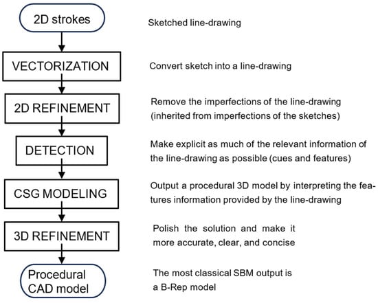
Figure 2. Main stages in SBM.

In principle, there are two classical approaches to deal with hidden edges in SBM. In the first, the user creates a natural drawing and then the system tries to automatically infer the back of it (which is not provided by the user). In the second, the user draws a wireframe representation of the solid shape without distinguishing that hidden from visible edges. Both are drawn as solid lines. Reconstruction approaches cannot rely on the visibility of the edges, which is generally unknown.

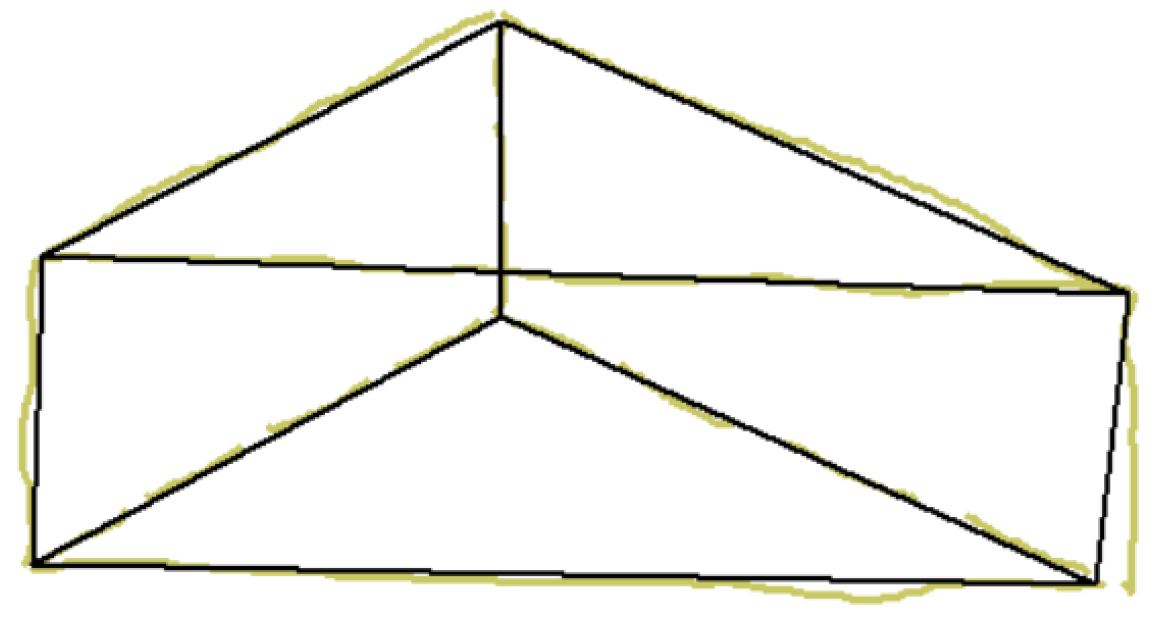
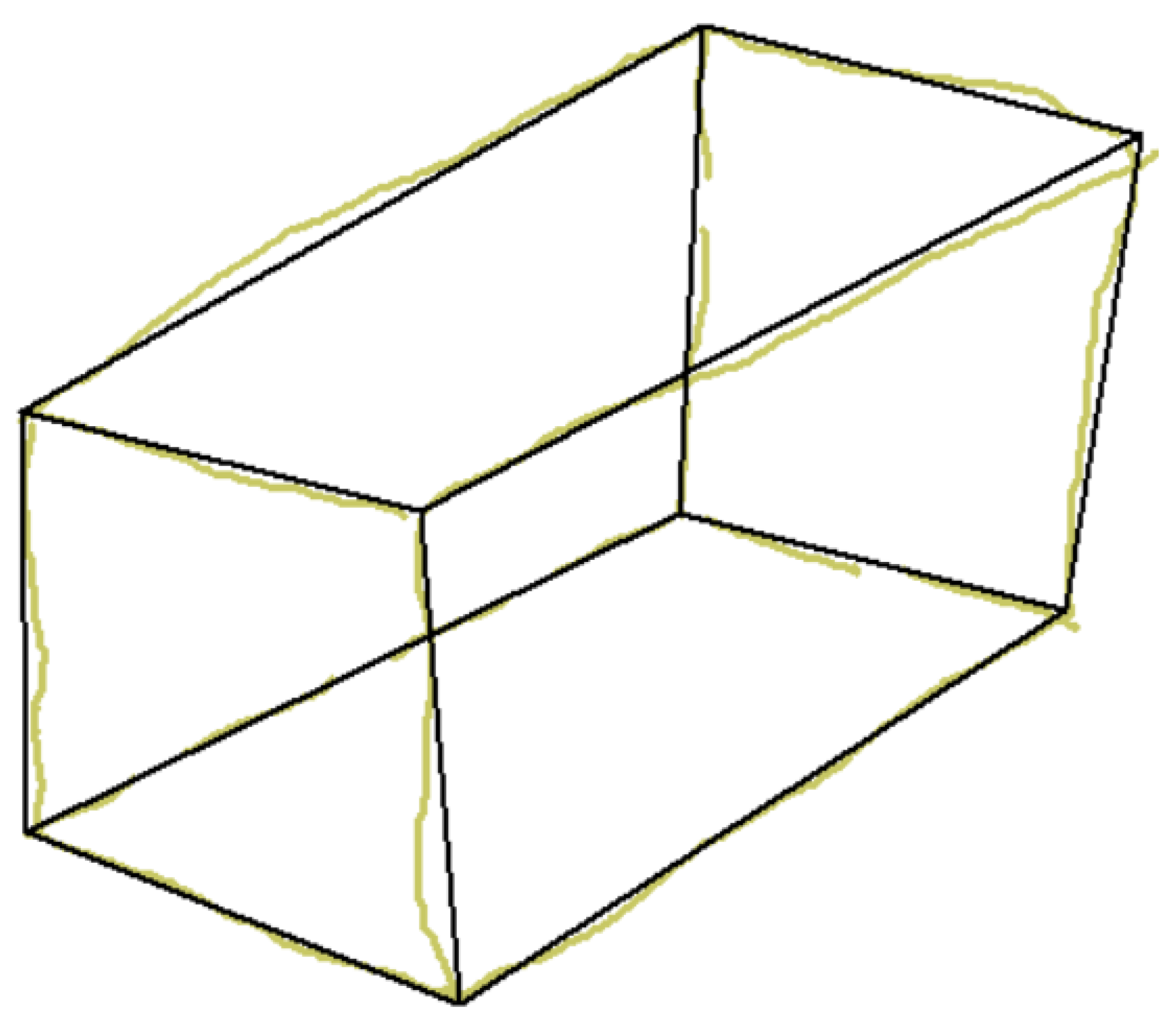
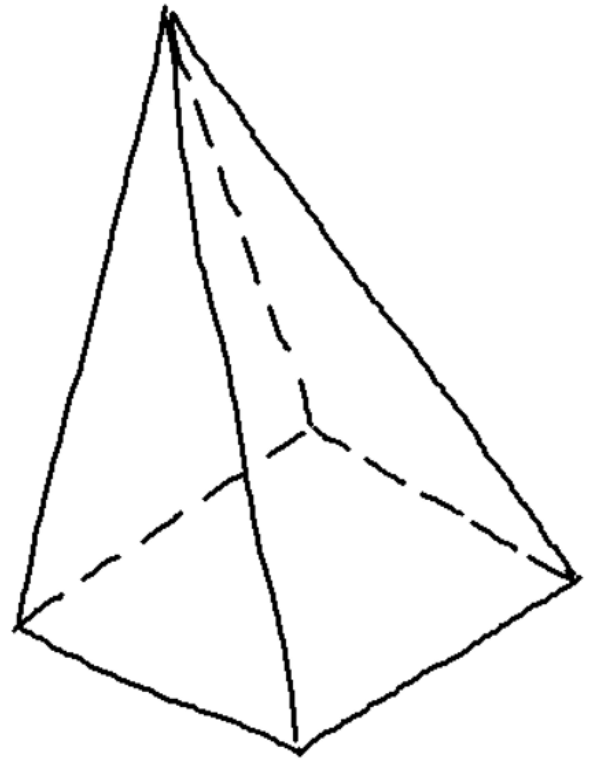
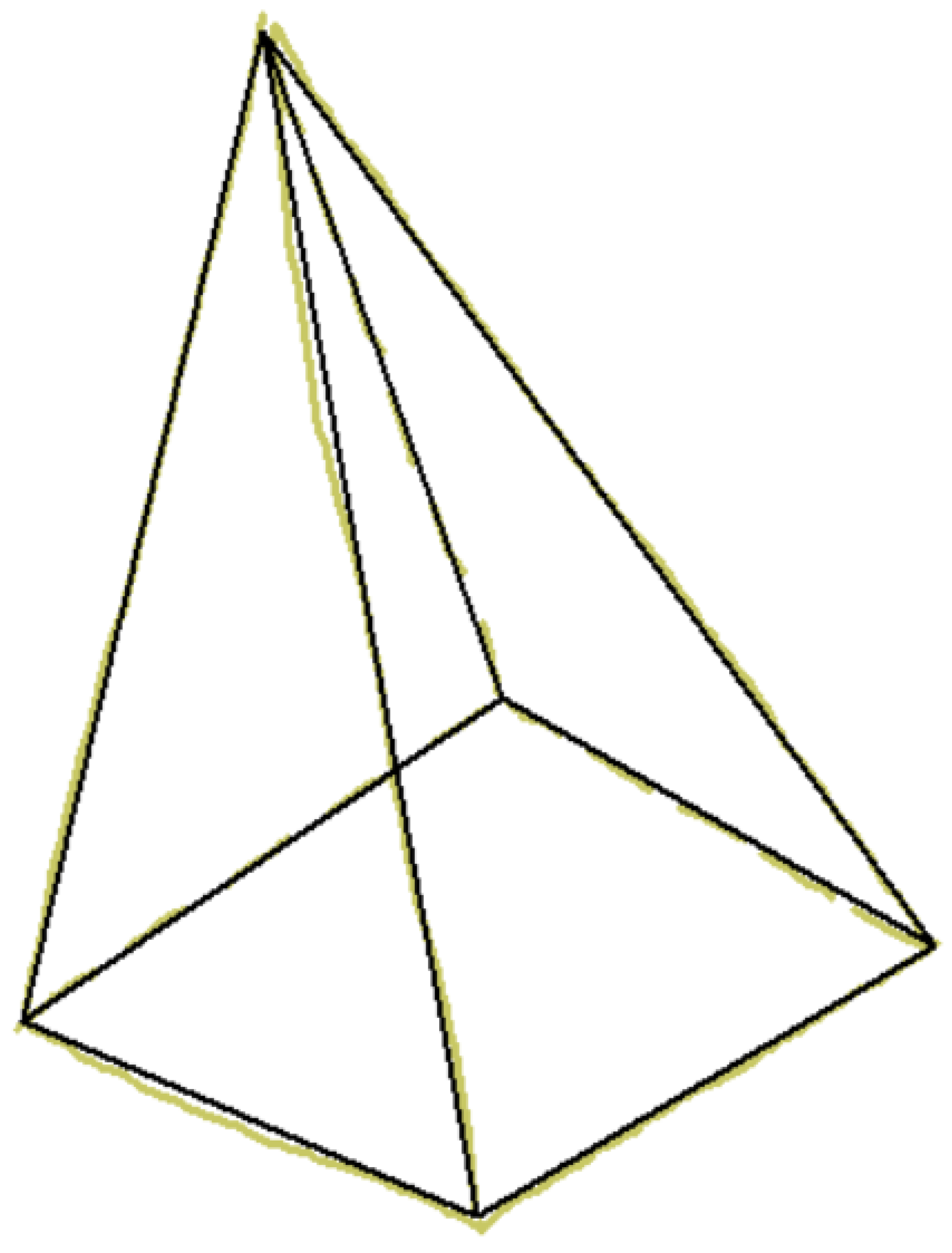
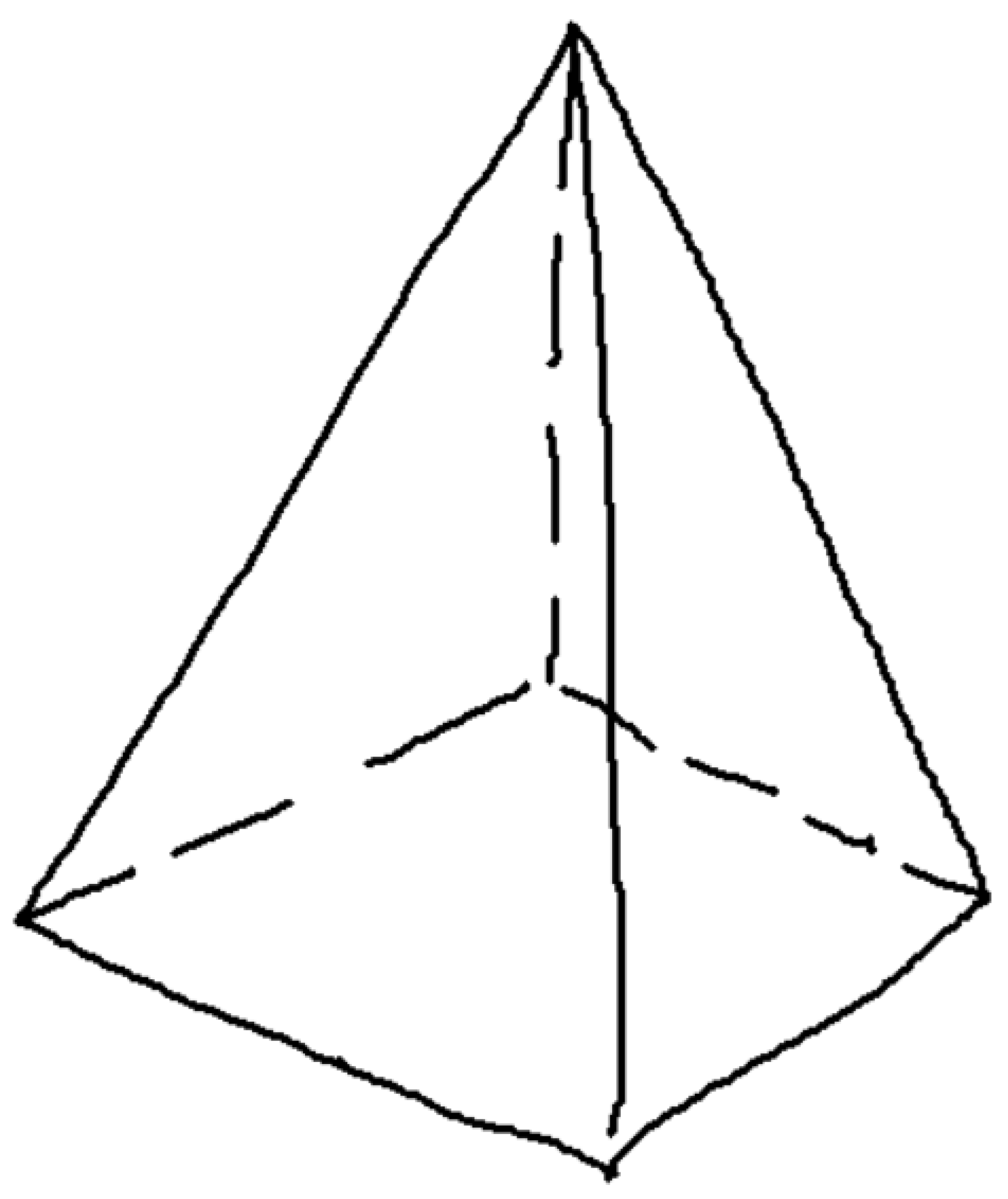
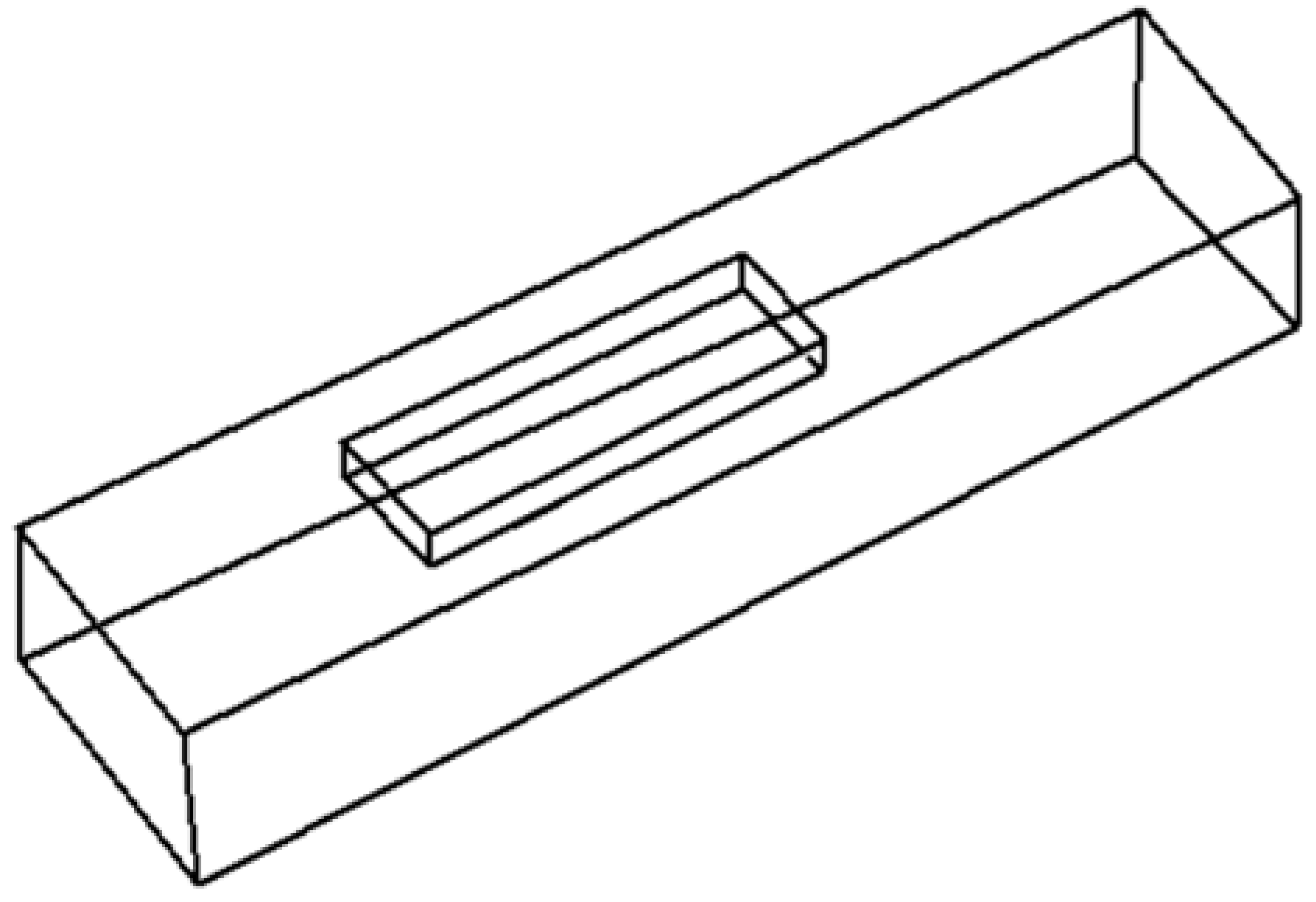
There is, however, a third alternative. A common artifact that is successfully used to convey information of the back of an object while increasing the perceptual sensation of volume involves the use of dashed lines to represent surfaces, edges, or corners of objects that are hidden from view (Figure 3).

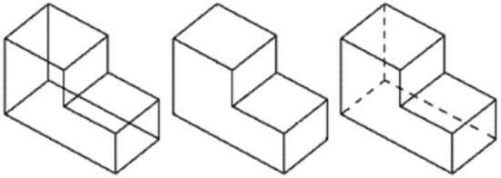
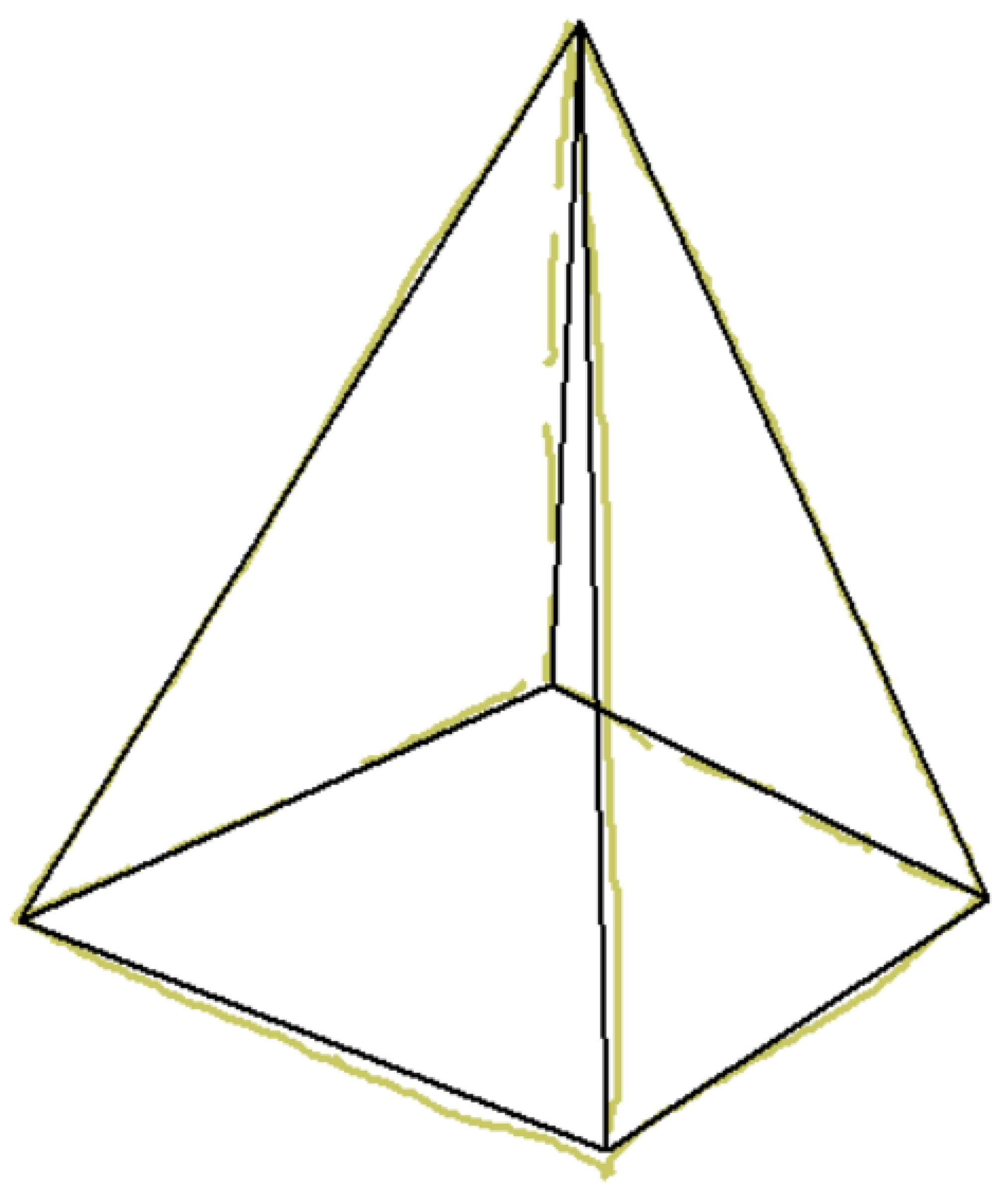
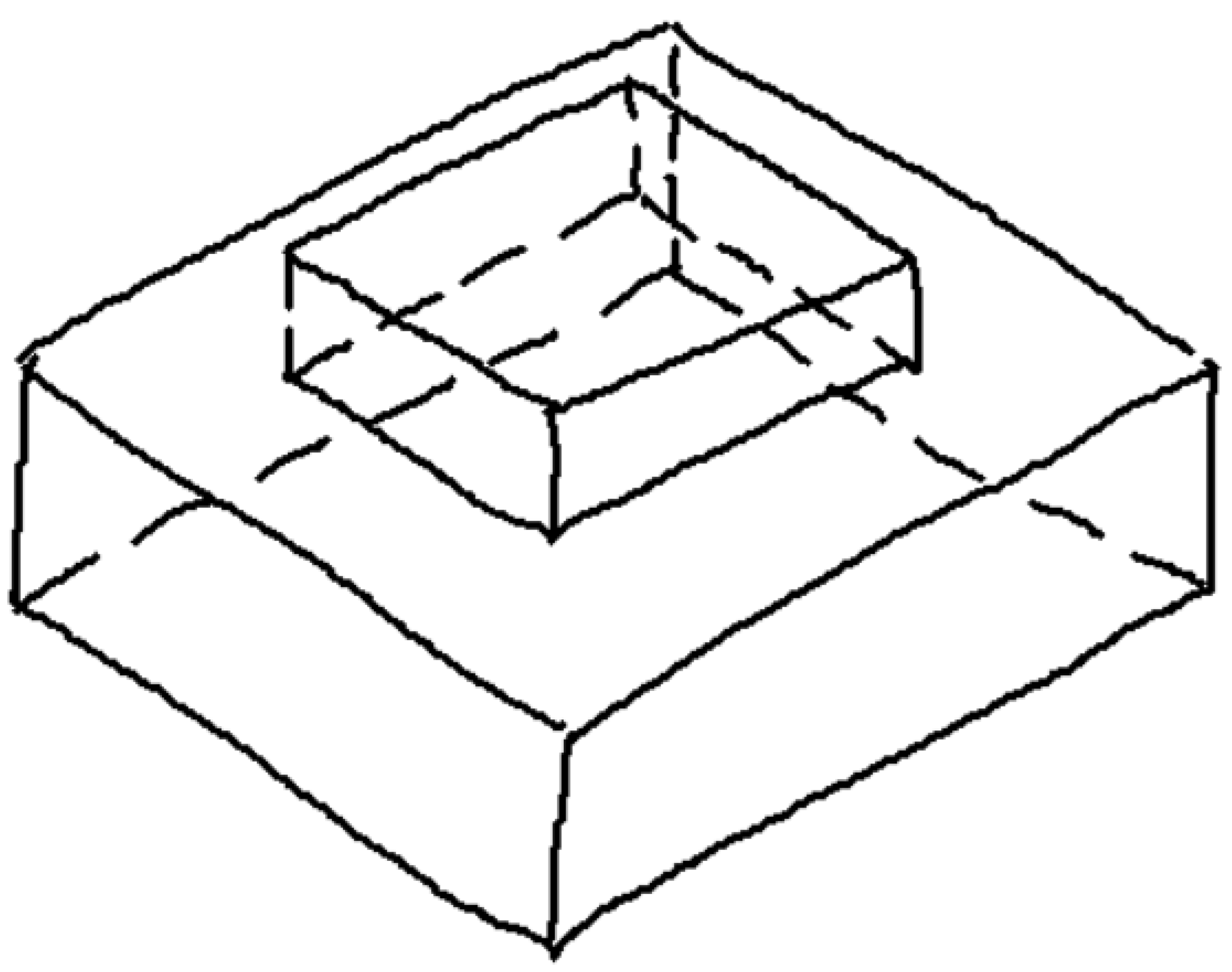
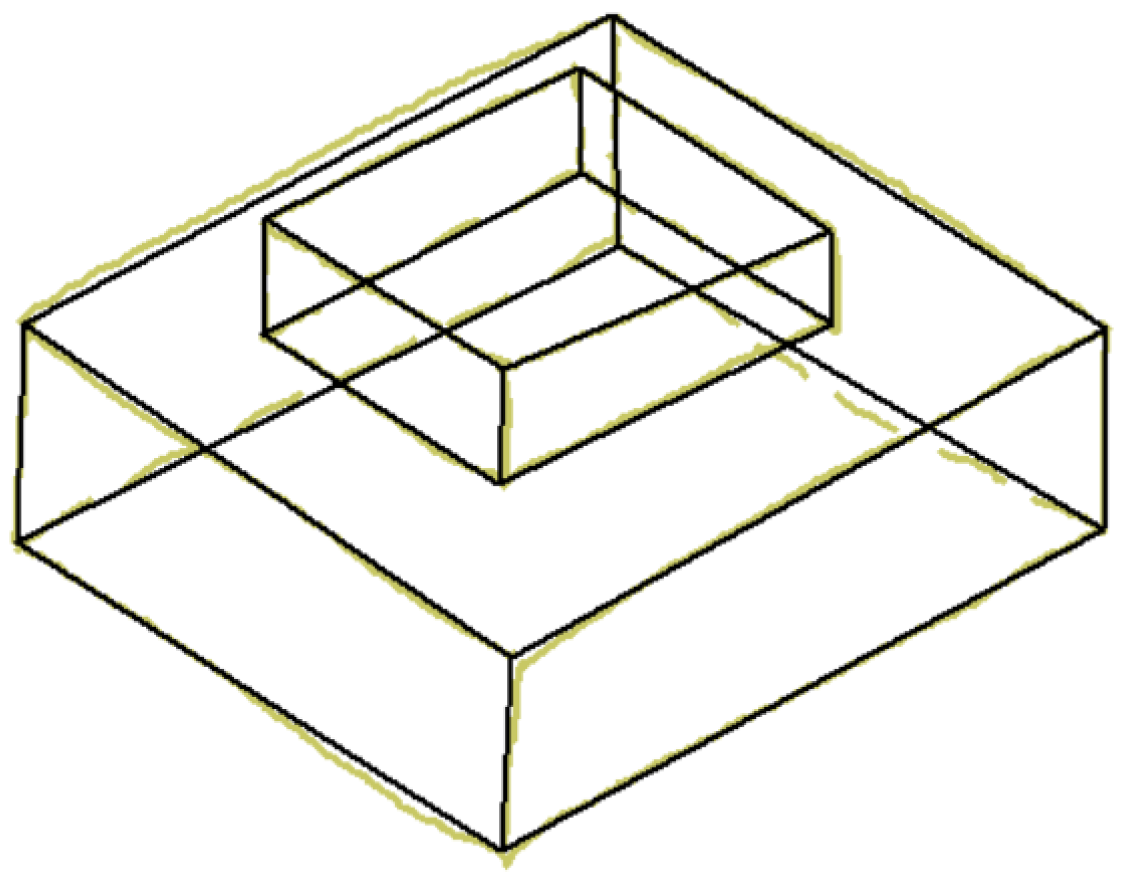
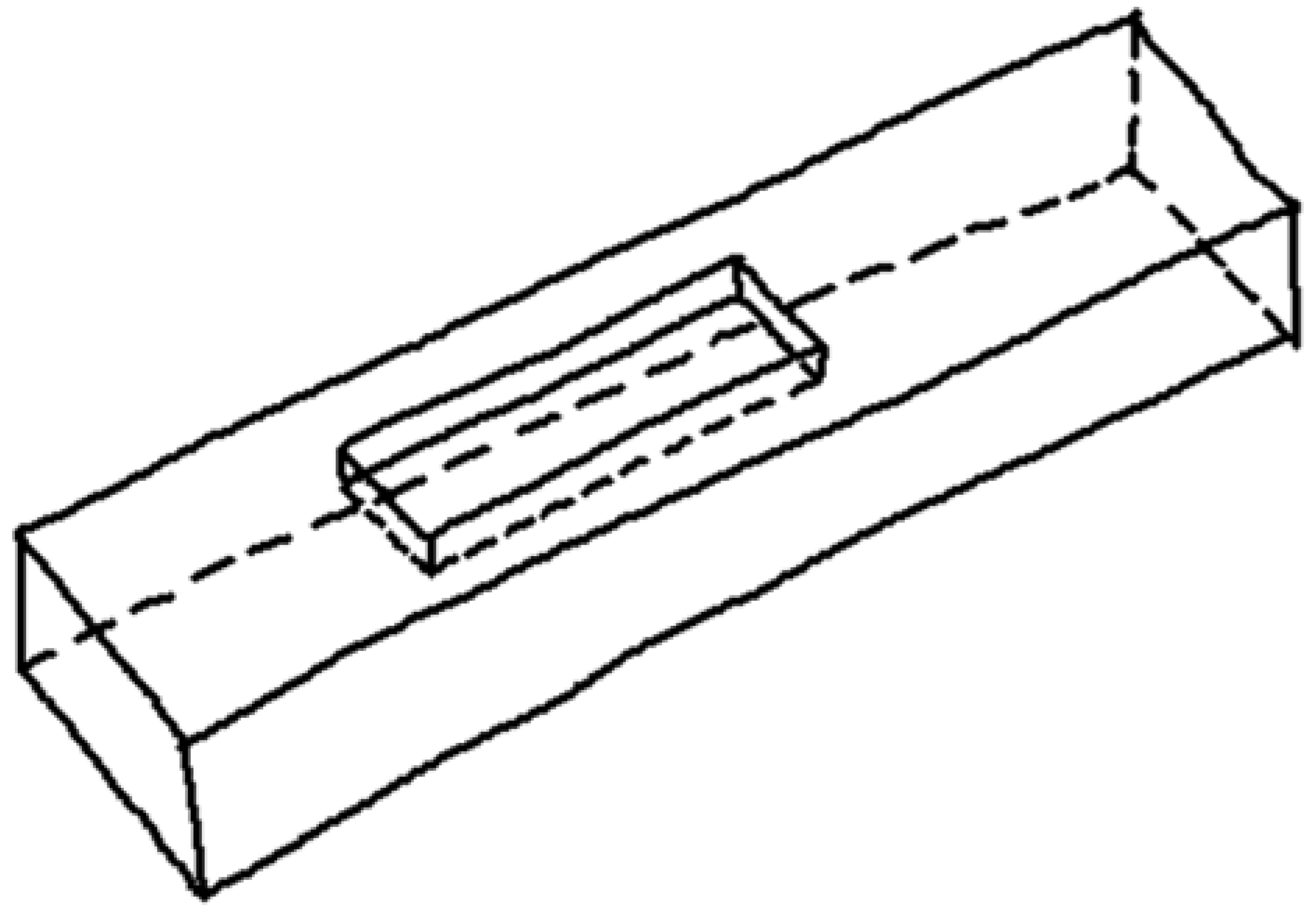
Figure 3. Wireframe (left), natural (center), and hidden lines (right) in isometric line-drawings.

A review of all three approaches concludes that drawing with hidden lines communicates higher-level geometric information more effectively than the other two approaches. However, it has not been explored extensively, presumably because detecting hand-drawn dashed lines remains an open problem.

Bonnici and Camilleri [7] contributed to finding hidden lines in a natural line-drawing, refining Varley’s original approach [8,9], and the approach provided by Kyratzi et al. [10,11,12]. All these approaches assume that the natural sketch is created in the most informative view, meaning that there is nothing on the ‘‘back of the sketch’’ that cannot be directly inferred from the visible part of it [11] and, most importantly, the user draws a sketch without hidden lines, which must be automatically inferred—and labeled as such—by the application. Therefore, dashed lines arise while parsing the sketch, but are missing at the input.

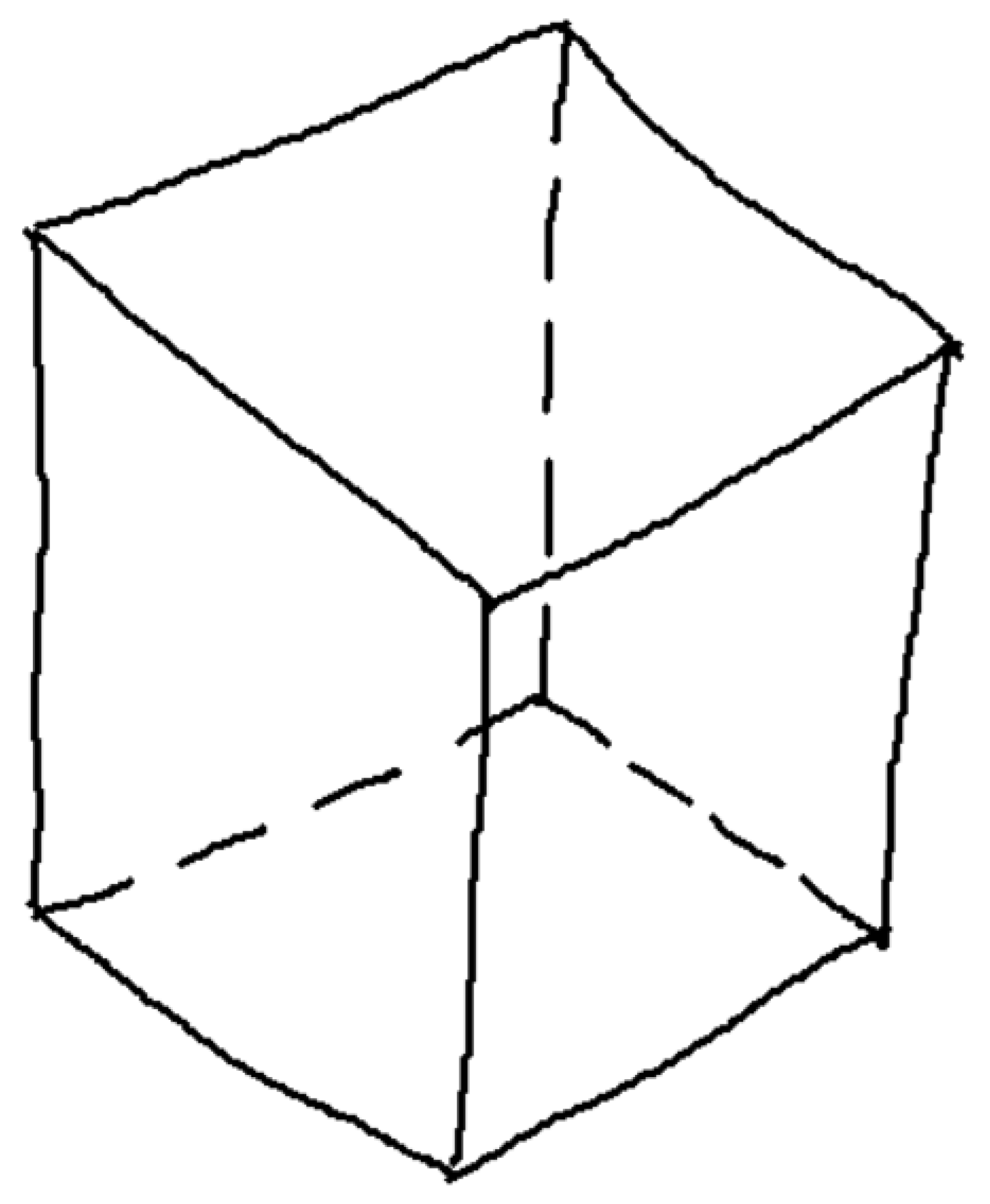
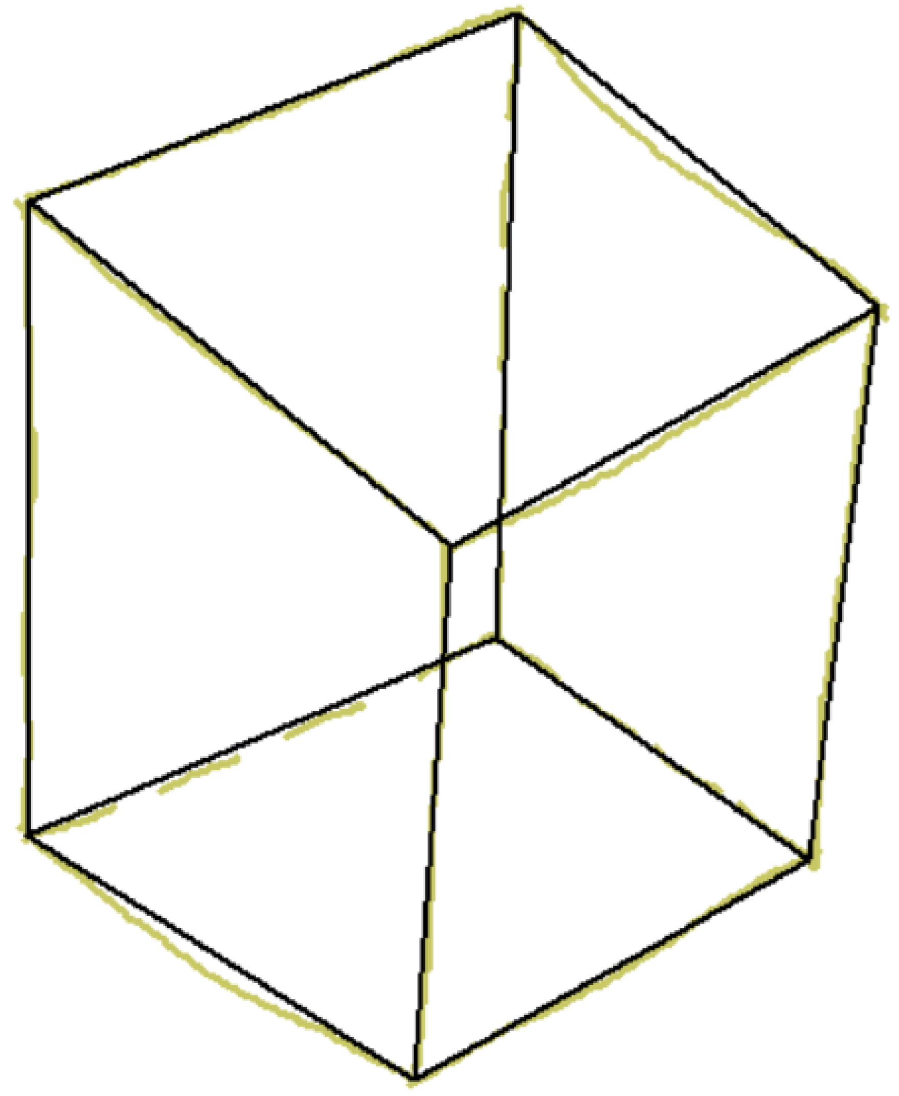
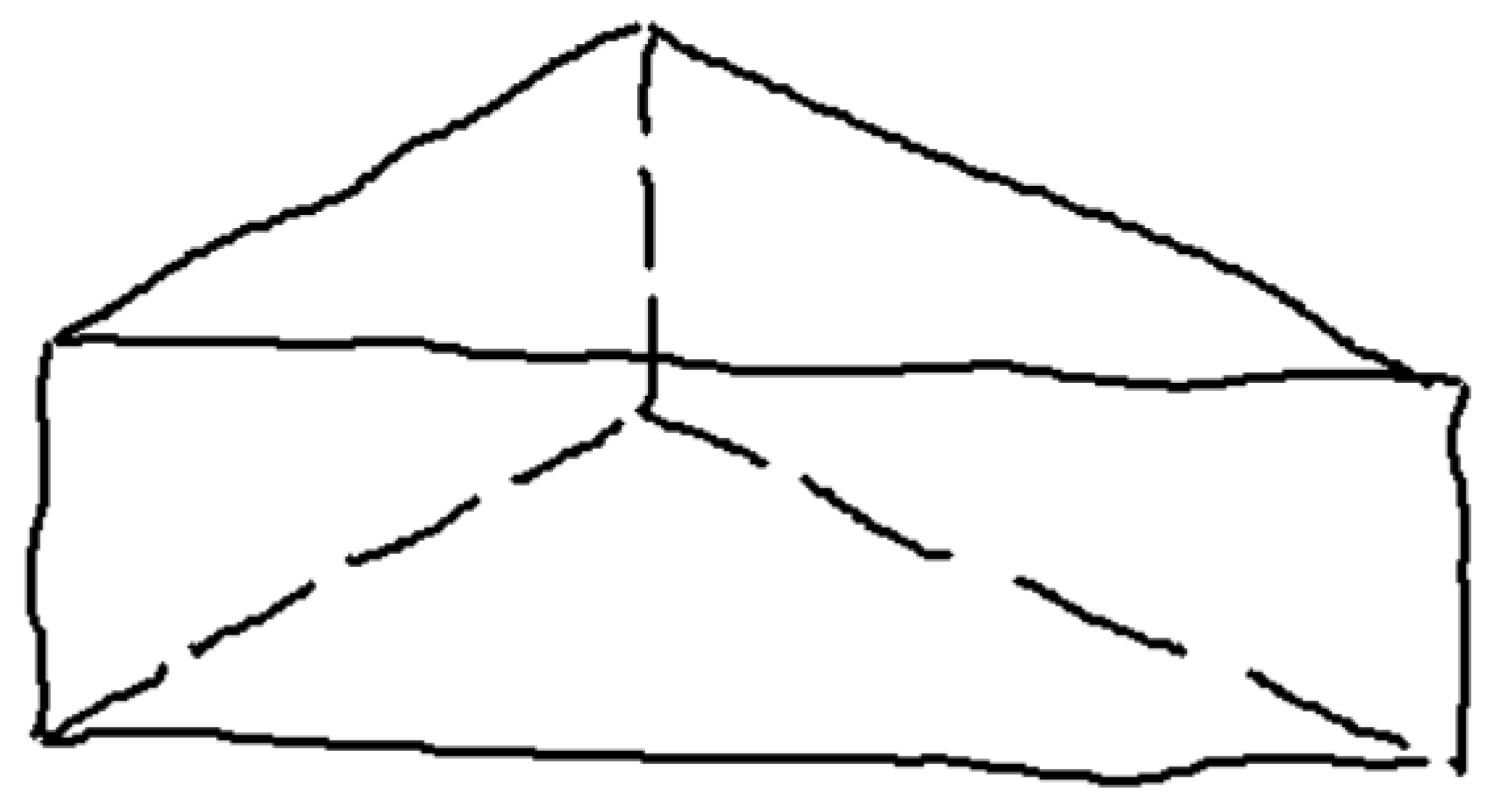
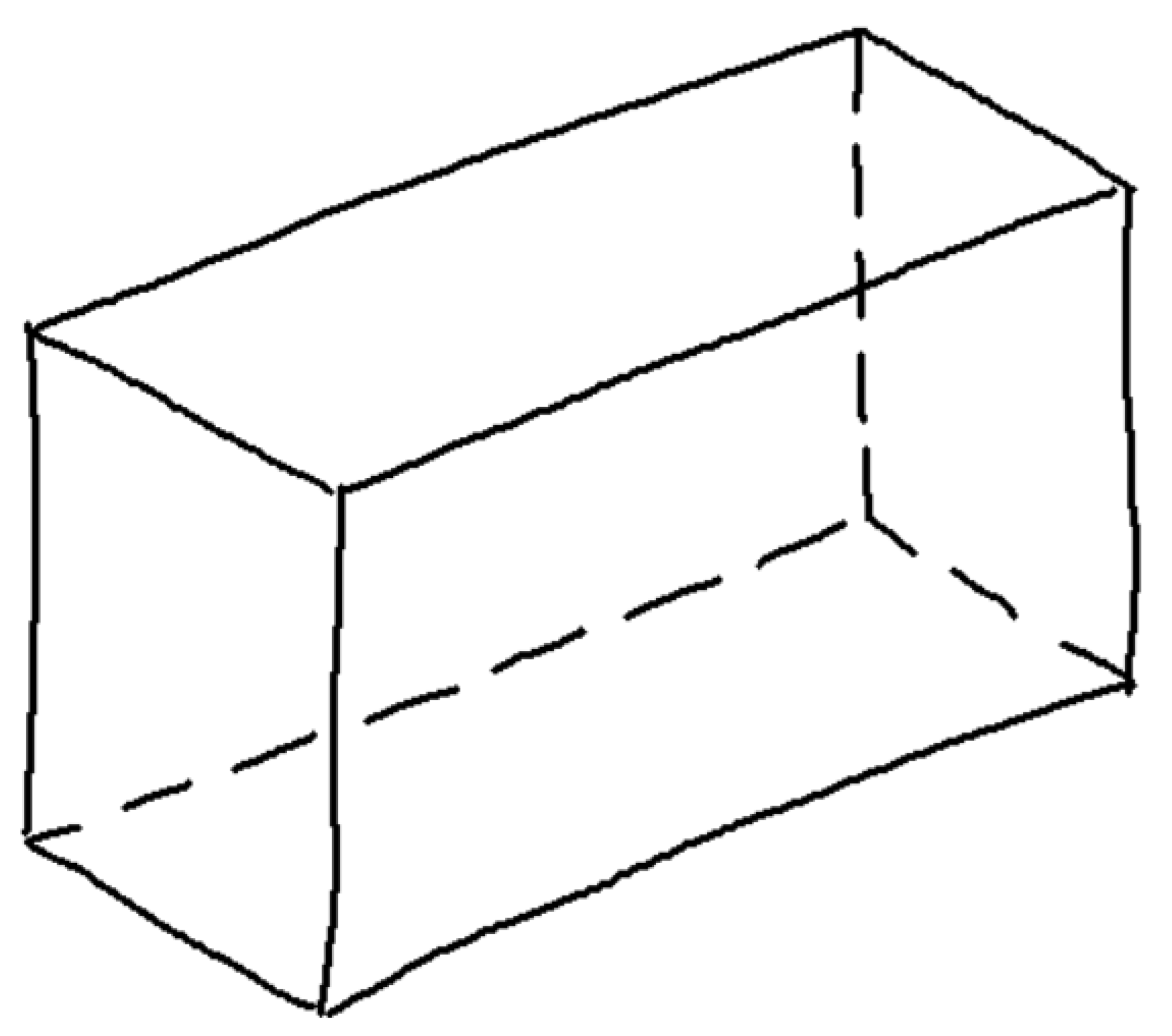
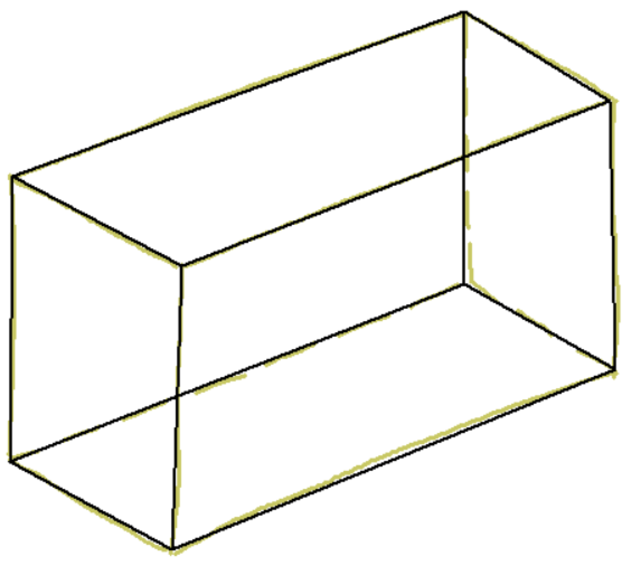
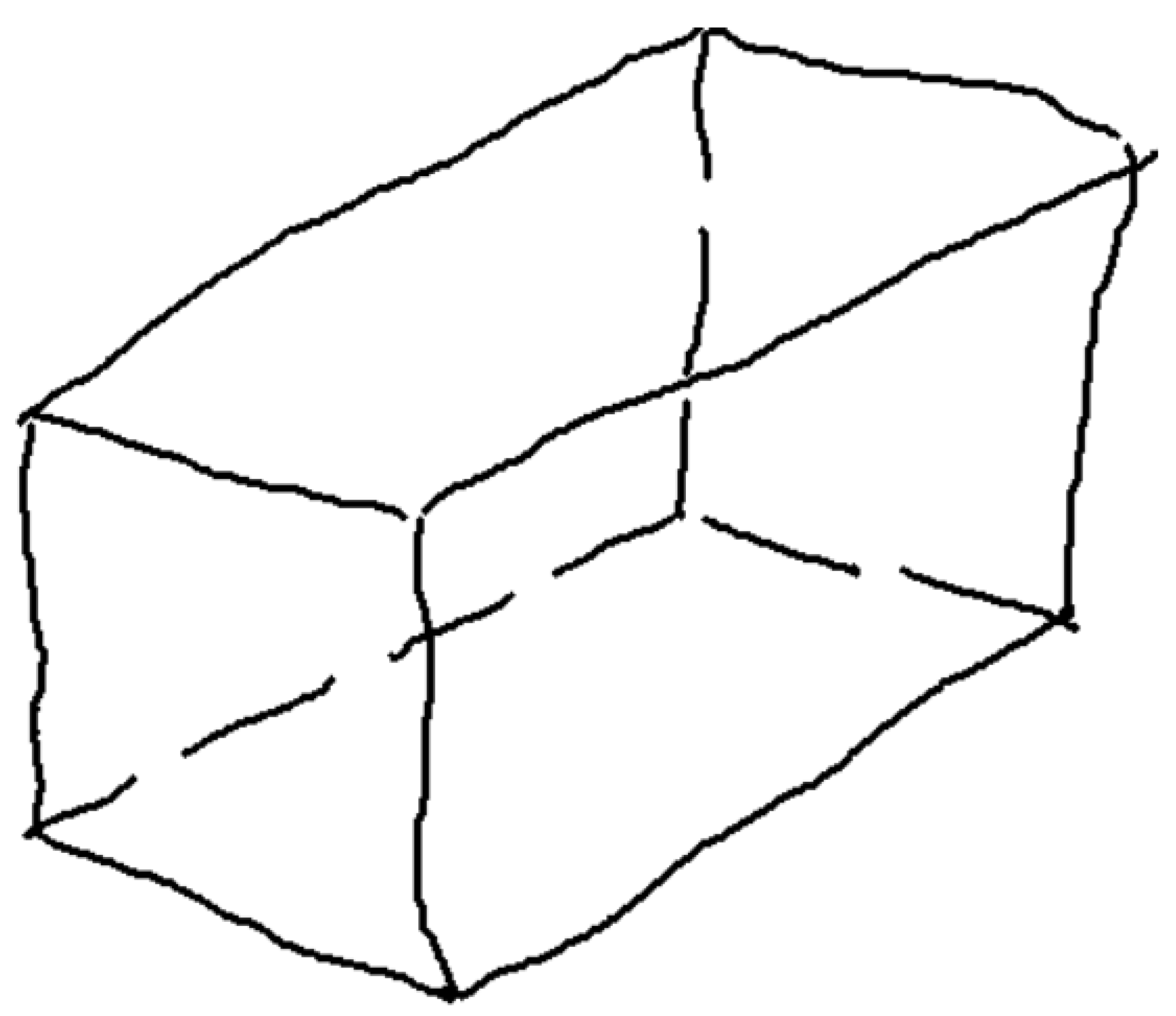
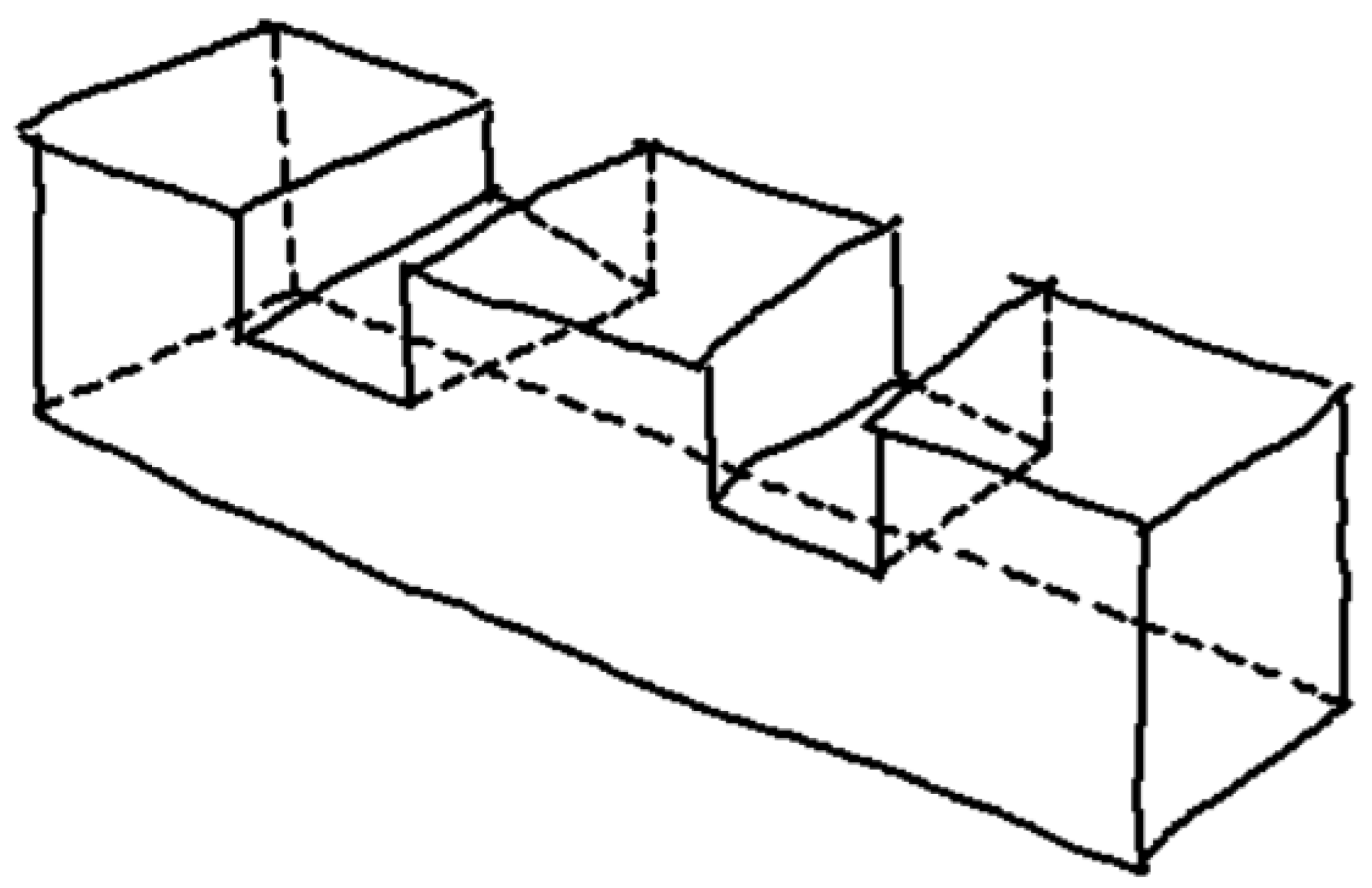
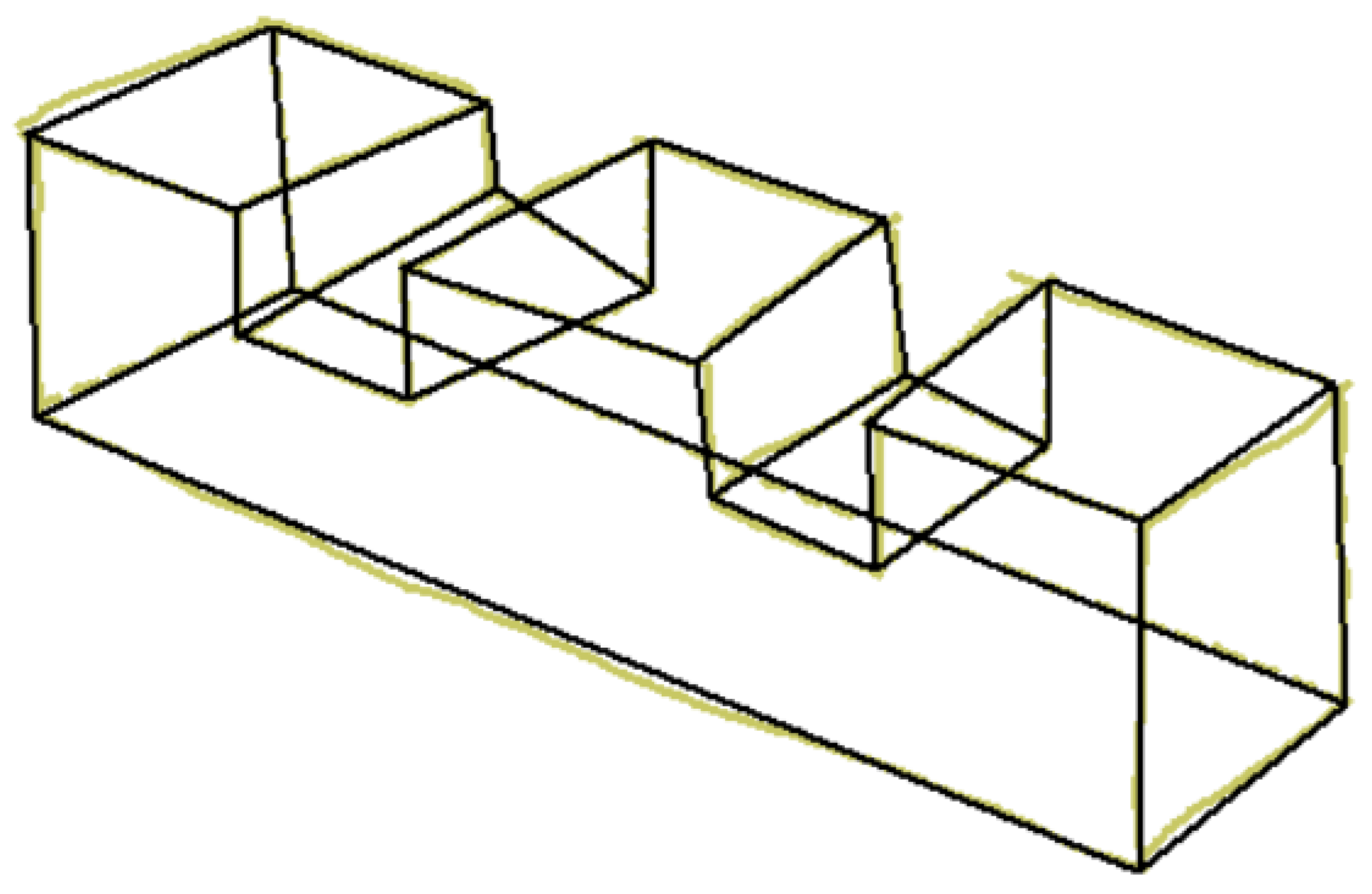
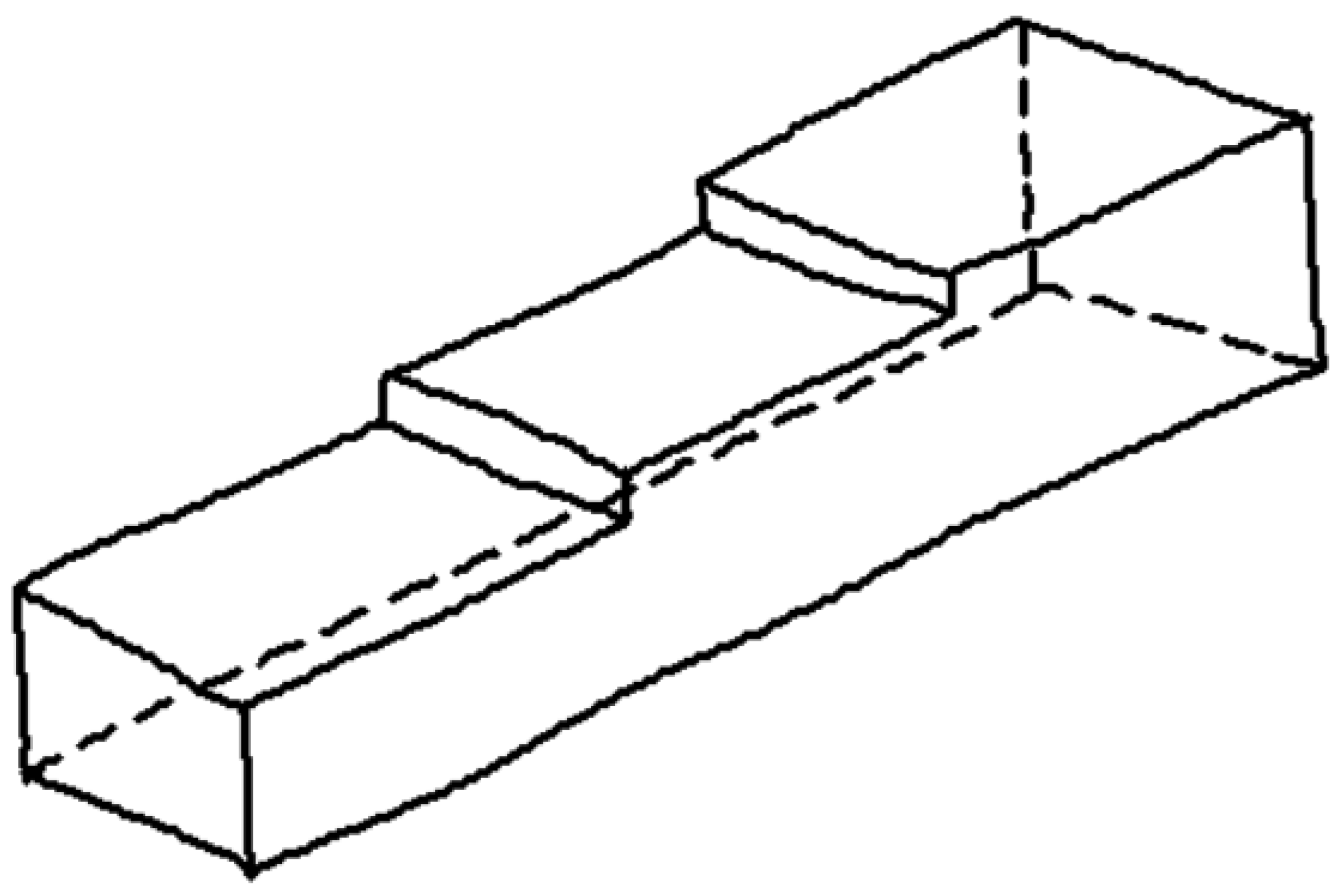
Wireframe drawings include hidden lines, but these are not identified as such. Consequently, the well-known ambiguity of wireframes (Figure 4) is commonly solved by reconstruction approaches that cannot rely on the visibility of the edges. As the recent review by Camba et al. shows [3], the reconstruction of wireframes operates by extracting alternative cues, such as faces and form features, while commonly avoiding trying to explicitly infer hidden edges.

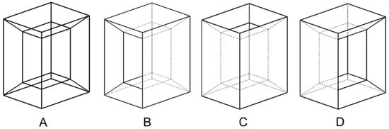
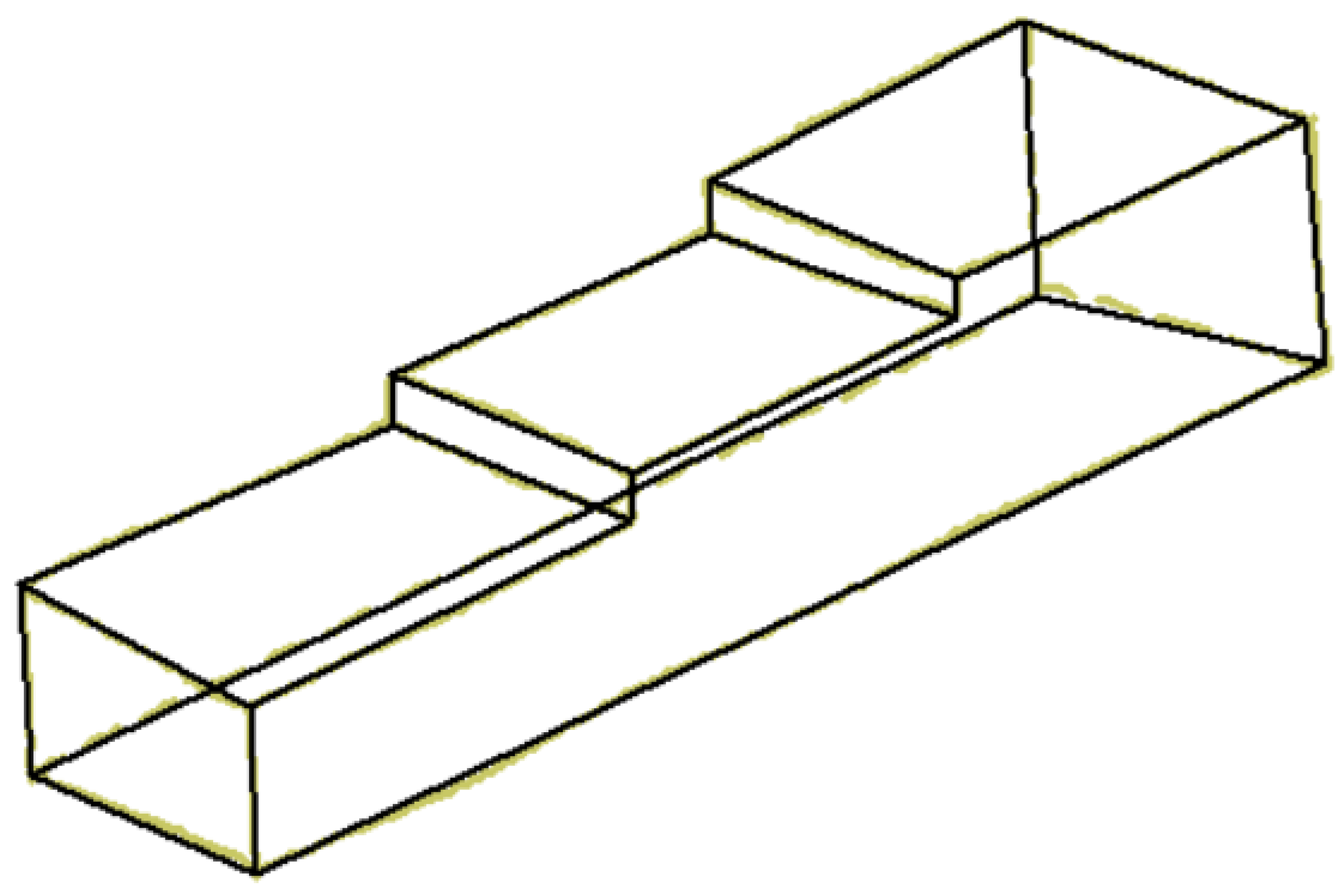
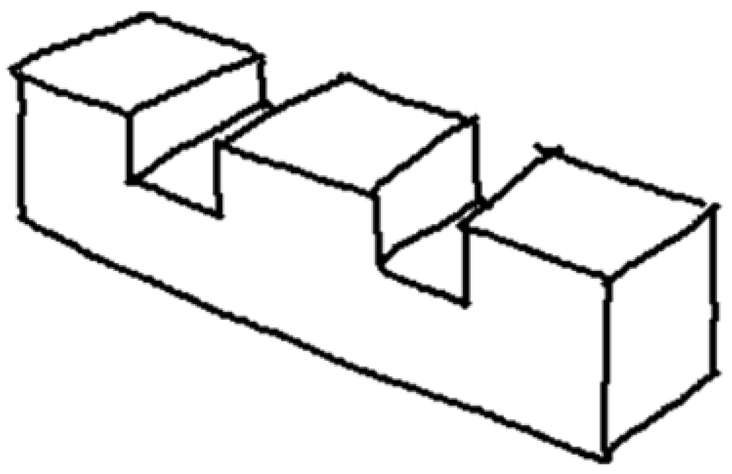
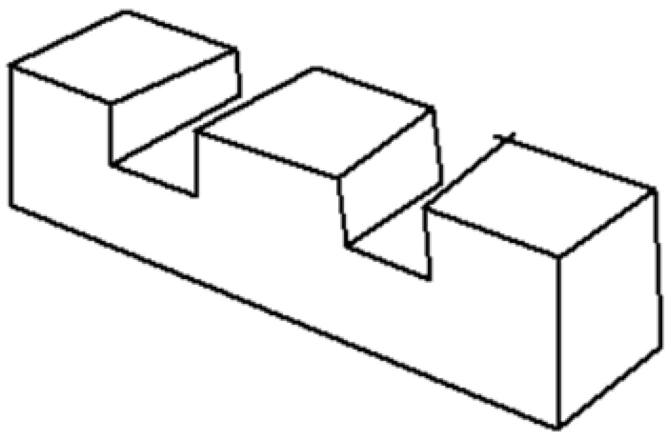
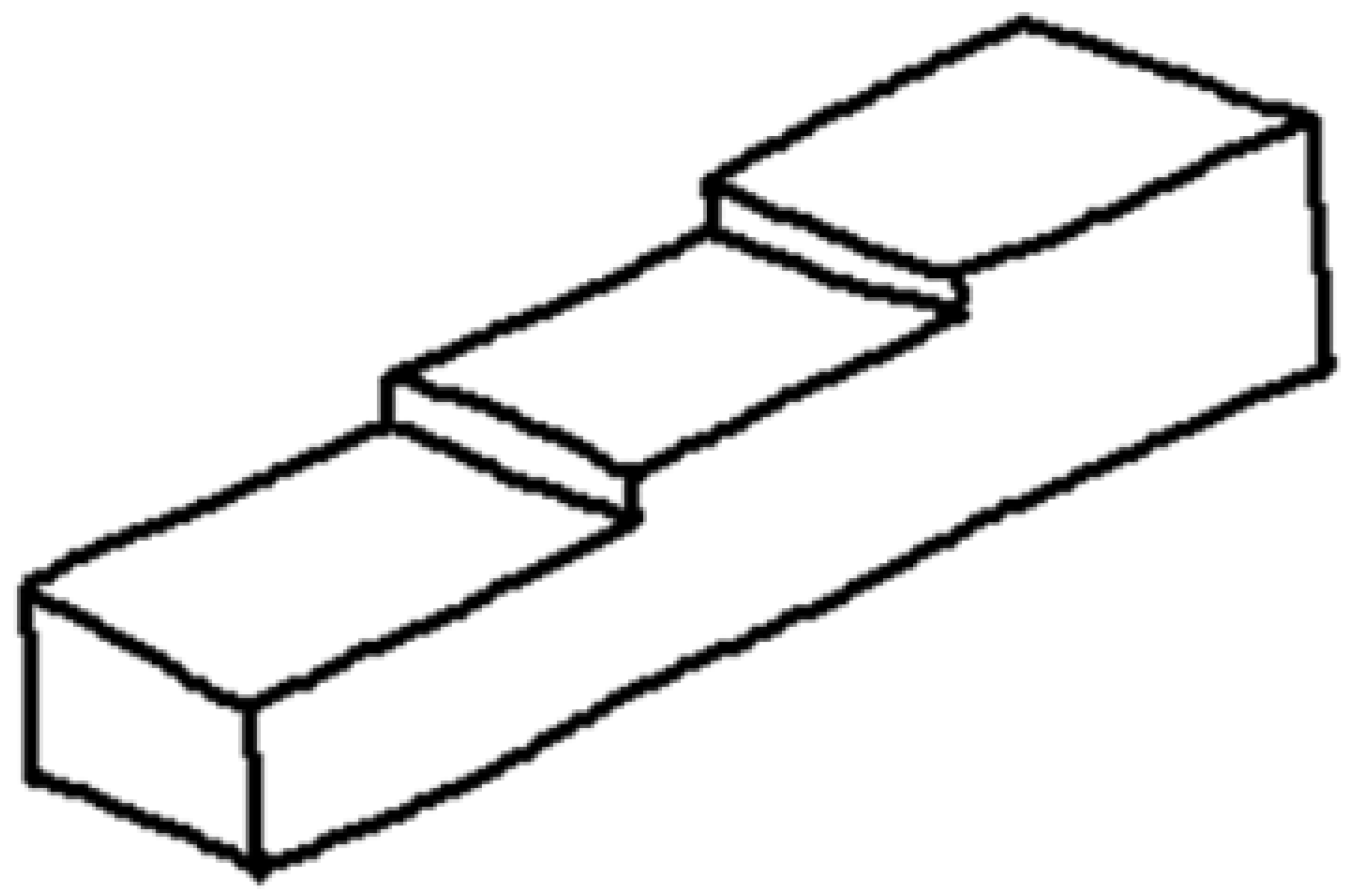
Figure 4. Wireframe model of polyhedral shape (A), with multiple volumetric interpretations in axonometric views (B–D).

To the best of our knowledge, the only publicly available algorithm to distinguish visible edges from hidden edges in wireframe drawings was published by Conesa [13]; it was an exhaustive search of all possible permutations of hidden/visible edges, or exhaustive permutations of hidden/visible faces (if faces were calculated in advance, for instance, following the approach of Varley et al. [14]).

Some algorithms to detect dashed lines are used for other purposes, like human–tablet interaction [15]. However, they depend on assumptions that may be acceptable only while interactively interpreting simple diagrams. For instance, forcing the user to draw the strokes consecutively enables a trivial procedure to detect dashed lines interactively. The algorithm must simply group the strokes in the order the user introduces them. The problem becomes much more challenging when there is no time information available (off-line interpretation) or when the user does not follow a particular sequence for drawing the strokes (repaired or beautified sketches).

The works of Lai and Kasturi [16] and Agam et al. [17] are some of the most representative of the initial works that were carried out in the field of the recognition and detection of dashed lines. Lai and Kasturi [16] attempted to recognize dashed lines by linking short and isolated bars in drawings and maps. Agam et al. [17] investigated the detection of dashed lines with straight and curved shapes on a pixel basis. Both have served as inspiration for subsequent work in the development of algorithms for image processing.

Finally, in recent years, the use of machine learning in image recognition has become widespread. In this regard, several methods with specific applications within engineering and design were developed. For instance, Fu and Kara [18] presented a method based on the use of a Convolutional Neural Network (CNN) as a trainable engineering symbol recognizer for network diagrams. The CNN can learn the visual characteristics of predefined symbol categories from a few diagrams provided by the user and a set of synthetically generated training samples. However, the method is not directly applicable to the recognition of dashed lines. Similarly, Moon et al. [19] introduced a method for recognizing lines and flow arrows in piping and instrumentation diagrams. The model was trained by a combination of image processing techniques and deep neural networks. Nevertheless, as the authors themselves acknowledge, the use of methods based in deep learning has limitations, such as the quality of the training dataset, which affects the accuracy of recognition results, as well as the difficulty in recognizing hand-drawn or non-standard symbols. In response to these limitations, there is growing interest among researchers in exploring hybrid models that integrate neural networks with symbolic artificial intelligence in different domains, such as the integration of visual language in AI systems [20].

For the reasons described above, we decided to employ and propose heuristic algorithms in this work. These types of algorithms are valuable and necessary for defining and developing more effective training for machine learning systems. Additional advantages of these algorithms are that they are more transparent than automated deep learning or machine learning methods, and they help understand human reasoning before automating it in a more modular or compartmentalized manner.

3. Vectorization Overview

Vectorization is a complex task, which commonly requires different stages aimed at producing 2D line-drawings, made of high semantic geometric elements, and intended as intermediate results to output 3D CAD models. The main stage involves fitting strokes into lines, i.e., skipping low-semantic-level geometric elements (typical output in raster to vector conversions) to identify the high-semantic-level primitives depicted by the strokes of a sketch. However, some sketch refinement is required:

• Some users tend to redraw the lines of the sketch by overlapping different strokes. This “sweeping the lines” produces overtraced strokes, which require grouping overtraces, to identify each single stroke/line, which was intended to represent.
• Some users sketch non-solid lines that are drawn as sets of consecutive strokes (for instance, by drawing hidden edges as dashed lines). Grouping non-solid strokes facilitates vectorization, while providing high-level information that may ease the subsequent reconstruction.
• There is no univocal relationship between strokes and lines, since some users do not pen-up when a stroke is created just to pen-down to start the following stroke that begins exactly where the previous one ends. Instead, they sketch a single stroke that depicts multiple lines. This “continuous” stroke produces poly-strokes that must be segmented by the suitable corner finding module, to bring up the different geometric primitives it contains.

In our approach, the first step of vectorization is to calculate fits of all the strokes. The second step involves grouping the overtraced strokes. A set of strokes is replaced by a single stroke that encompasses them all. The fit of the resulting stroke is calculated and the strokes that have been grouped are removed from the sketch. The third step involves grouping non-solid strokes. The strokes of all the dashes are replaced by one single stroke that encompasses all of them (and the fit of this resulting stroke is calculated). The strokes that do not fit well with either straight lines or ellipse arcs are segmented, and their segments are fitted, thus obtaining an initial vectorized drawing, which is later refined.

From the overall vectorization process, only the stage of grouping non-solid lines is studied here. Readers interested in fitting are recommended to explore the works by Plumed et al. [21,22], Ku et al. [23], and Bartolo et al. [24], which introduced overtrace detection and clustering. Wang et al. have also contributed with interesting advances [25,26,27] and the work by Xiong and LaViola [28] is useful to understand the problem of detecting corners.

4. Non-Solid Line Clustering

Algorithm 1 identifies potential dashed strokes by chaining dashes that are short, isolated, consecutive, and aligned. The general flow is explained by the next pseudocode:

Algorithm 1. Dashed Stroke Identification Algorithm

Input: Set of strokes in a sketch drawing. Output: Identified dashed stroke chains. 1: Initialization:

• Put short and isolated strokes in a list of candidate dashes.  • Label dashes of the list as non-visited.

2: Main Loop:

• While there exist non-visited candidate dashes:

2.1: Select one non-visited candidate dash from the list. 2.2: Start a new chain with the selected candidate dash. 2.3: Label the candidate dash as visited. 2.4:. Explore adjacent candidate dashes:

• For each candidate dash not yet visited:       • If the current candidate dash is consecutive to the chain:           • Evaluate its consecutiveness merit.           • If the current candidate dash is aligned with the chain:               • Evaluate its alignment merit.               • Evaluate its overall dash merit by combining                 consecutiveness and alignment merits.               • If the dash merit is greater than the current best merit:                   • Select the current candidate dash as the best-                     continuation.    • While a best-continuation was found:       • Add the best-continuation dash to the chain.       • Label the best-continuation dash as visited.       • Repeat the exploration from step 2.4.

2.5: Merge all dashes of the chain into a common line if the chain contains more than one dash. 2.6: Label all dashes of the chain as visited. 2.7:. Repeat the main loop until all candidate dashes have been visited. End Algorithm

Terms like “short”, “isolated”, “consecutive”, and “aligned” pose computational challenges due to their unprecise nature. They are qualitative criteria that depend on a mixture of geometric and perceptual concepts. Therefore, it is important to highlight that the algorithm depends on certain configuration parameters that must be tuned for the dashed stroke search as they significantly impact the efficiency and quality of the process. When used along this section, these parameters are denoted in bold and italics for easy identification. They are further analyzed in Section 5.

Next, we first detail the input data; then, we describe the criteria to select candidate dashes. We subsequently describe the recursive procedure to search for chains of consecutive dashes, to finally explain the output information.

4.1. Input Data

The input to our algorithm is a sketch represented as a set of strokes. These strokes are hand-drawn lines obtained by sampling scribbled lines by way of a set of consecutive nodes that are automatically sampled by the device (mouse, pen, etc.) between the pen-down and pen-up movements. The result is a set of ordered points, which are connected by segments to approach the original scribble.

Along with the sketch, we input the endpoints of segments that best fit their strokes. This information was calculated in advance ([21,22]). For this purpose, we employ a regression fit, a method that is slower than others but less susceptible to sketch inaccuracies, which can be critical for short strokes, which are commonly found in dashed lines. The fitted segment is determined by the regression line encapsulating the stroke and delimited by the points on the regression line closest to the tips of the stroke (refer to Figure 5 for an illustration). The implementation of the typical line-of-best-fit algorithm considers the need to swap coordinates for lines with a slope greater than 1, preventing the well-known issue of regression failure for vertical lines. For each stroke, the fitting algorithm calculates

Figure 5. Fitting one stroke to its regression line.

• Coordinates of the initial tip of the fitting segment (<TipBegin (x, y)>);
• Coordinates of the final tip of the fitting segment (<TipEnd (x, y)>);
• Length of the segment (<Length>);
• Orientation (angle in radians).

4.2. Obtaining Candidate Dashes

To enhance the efficiency of the search process, the algorithm first discards those strokes that are implausible dashes, following these steps:

• Exclusion of Long Strokes:

Excessively long strokes are excluded as candidate dashes, as SBM dashed lines typically represent hidden edges, which can only be hidden by faces delimited by edges that are necessarily larger than the dashes. The algorithm determines the length of the longest segment in the sketch, denoted as <MaxLength>. Subsequently, a threshold value <TrimLength> is calculated as a percentage of <MaxLength>:

$$TrimLength=MaxLength ·\mathit{D}\mathit{a}\mathit{s}\mathit{h}\mathit{S}\mathit{i}\mathit{z}\mathit{e}\mathit{M}\mathit{a}\mathit{x}$$

(1)

where DashSizeMax has a default percentage of 50%. Segments exceeding the length of <TrimLength> are discarded and labeled as non-visitable.

2.

Discarding non-isolated strokes:

Candidate stroke tips must maintain a significant distance from neighboring tips. The valence of each tip is then calculated to identify potential shared vertices, avoiding collinearity. Closeness is determined by a threshold relative to stroke size, calculated as

$$Threshold=\left|Segment length\right|·\mathit{I}\mathit{s}\mathit{o}\mathit{l}\mathit{a}\mathit{t}\mathit{e}\mathit{d}\mathit{T}\mathit{i}\mathit{p}\mathit{T}\mathit{h}\mathit{r}\mathit{e}\mathit{s}\mathit{h}\mathit{o}\mathit{l}\mathit{d}$$

(2)

The default value of IsolatedTipThreshold is 25% of the dash length. The algorithm then identifies endpoints near stroke tips, excluding collinear strokes. If both tips have a valence > 0, the stroke is discarded as dashed and marked as non-visitable.

3.

Assessment of stroke similarity:

The algorithm temporarily excludes strokes that significantly deviate from the average stroke length. At the start of each search iteration, the average length of the remaining candidate strokes <avgLength> is recalculated. Based on the principle of similarity, the algorithm assumes that only similar dashes belong to a single dashed stroke. It uses the average length of remaining candidate strokes, <avgLength>, to establish the length range for currently visitable dashes:

$$DashLengthMin=\frac{avgLength}{\mathit{D}\mathit{a}\mathit{s}\mathit{h}\mathit{S}\mathit{i}\mathit{z}\mathit{e}\mathit{S}\mathit{h}\mathit{o}\mathit{r}\mathit{t}\mathit{R}\mathit{a}\mathit{n}\mathit{g}\mathit{e}}$$

$$DashLengthMax=avgLength ·\mathit{D}\mathit{a}\mathit{s}\mathit{h}\mathit{S}\mathit{i}\mathit{z}\mathit{e}\mathit{L}\mathit{o}\mathit{n}\mathit{g}\mathit{R}\mathit{a}\mathit{n}\mathit{g}\mathit{e}$$

(3)

where DashSizeShortRange is the number of times that a stroke should be shorter than the average dash to be excluded (default is 5 times shorter). DashSizeLongRange is the number of times that a stroke should be longer than the average dash to be excluded (default is 2.5 times longer). Candidate strokes that fall outside the range [DashLengthMin, DashLengthMax] are temporarily discarded and labeled as currently non-visitable. These strokes may become visitable later as the algorithm progresses and adjusts the average length based on remaining non-visited dashes. Hence, these parameters must be recalculated each time a candidate dashed line is created and the search for remaining dashed strokes is relaunched. Since shorter strokes are prioritized for visitation, these parameters tend to increase as the search progresses and the short strokes are gradually grouped together.

4.

Evaluation of gap consistency:

Following again the perceptual principle of similarity, the algorithm assumes that only dashes that are separated by similar gaps may belong to a single dashed stroke. Therefore, <avgLength> is used to calculate the gap range for currently visitable dashes, which is computed as follows:

$$DashGapMin= \frac{avgLength}{\mathit{D}\mathit{a}\mathit{s}\mathit{h}\mathit{G}\mathit{a}\mathit{p}\mathit{S}\mathit{h}\mathit{o}\mathit{r}\mathit{t}\mathit{R}\mathit{a}\mathit{n}\mathit{g}\mathit{e}}$$

$$DashGapMax=avgLength·\mathit{D}\mathit{a}\mathit{s}\mathit{h}\mathit{G}\mathit{a}\mathit{p}\mathit{L}\mathit{o}\mathit{n}\mathit{g}\mathit{R}\mathit{a}\mathit{n}\mathit{g}\mathit{e}$$

(4)

where DashGapShortRange specifies how much shorter the fictitious segment connecting two consecutive tips must be than the average dash to be excluded (default: 10 times shorter). DashGapLongRange indicates how much longer this segment must be than the average dash to be excluded (default: 2 times longer). Subsequently, candidate dashes with gaps outside the range [DashGapMin, DashGsapMax] are temporarily discarded and labeled as currently non-visitable.

5.

Straightness check:

Straightness of dashes is evaluated after the chain is complete. The merit of each stroke (MeritDashLine[i]) is calculated by following the approach by Plumed et al., controlled by three parameters, as explained in [21]: LineTolMin defines the narrow tolerance band for optimal straight strokes, LineTolMax defines the wider tolerance band for acceptable straight strokes, and LineSmoothPenalty reduces deviations to maintain stroke shape integrity. The merits reach a value of 1 if the shape of the stroke closely resembles a straight line (inside the narrow tolerance band) and 0 when there is a significant deviation beyond the relaxed band. Those merits are compared against the user-defined parameter DashMinMeritLine (which defaults at 0.25). Each dash is labeled as straight-enough or non-straight, and the chain must possess more than a minimum threshold of MaxNonStraightDashes, a percent of the minimum number of straight dashes (default is 40%). This filter, described in Algorithm 2, is used to avoid the acceptance of chained irregular strokes, while tolerating a moderate level of imperfection in the single dashes of a dashed line (Figure 6).

Algorithm 2. Detection of non-straight chain
1: for (long i = 0; i < Chain.size; i++);   2: if (MeritDashLine[i] < DashMinMeritLine) then     3: NonStraight++;   4: end if 5: end for 6: if (NonStraight > MaxNonStraightDashes · Chain.size) then 7: reject Chain; 8: end if

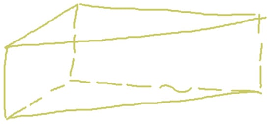
Figure 6. Non-straight dash in context.

The algorithm detects non-straight chains based on the evaluation of individual dash merits compared to a predefined threshold.

4.3. Chaining DASHED STROKES

Chains of strokes are calculated recursively by adding new strokes that must meet the following criteria: (1) they should not have been previously visited (which is easily achieved by labeling the dashes already visited); (2) their length must align with the current range (candidate dashes must fall inside the range [DashLengthMin, DashLengthMax], as explained previously); (3) they must be consecutive to one of the tips of the current chain of dashes (without overlapping or being too distant), by falling inside the range [DashGapMin, DashGapMax], as explained earlier; and (4) they should exhibit a similar orientation to previous dashes, within a specified angle and offset. We next describe in detail the procedures that guarantee that the last two conditions are satisfied.

• Consecutiveness verification:

The new stroke must be consecutive (continue or precede, not overlapping) to the current chain (which may contain more than one stroke). Furthermore, the gap, which represents the minimum distance between the new stroke[i] and the chain, as illustrated in Figure 7, must fall within the range defined by the calculated maximum and minimum gap, as per Equation (4). The decision is made following the Algorithm 3:

Algorithm 3. Consecutive stroke verification

1: gap = min(F0, F1, L0, L1); 2: if ((gap > DashGapMax) ||(gap < DashGapMin)) then 3:     Discard stroke[i] 4: end if

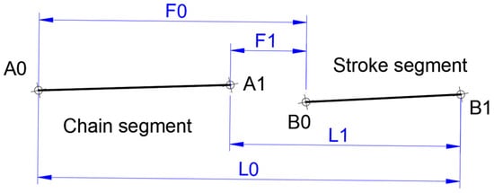
Figure 7. The gap is the minimum distance between tips of the chain and the new stroke.

The algorithm verifies the consecutiveness of strokes and checks if they fall within the defined gap range.

For valid gaps, their merit (meritGap) is calculated as a ramp function that equals 1 for a gap equal to the average gap, while it equals 0 for gaps equal to DashGapMin or DashGapMax (Figure 8).

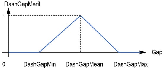
Figure 8. Gap merit ramp function.

• Alignment with current segment:

The new stroke should also be reasonably aligned with the current chain. To perform this verification, the thresholds derived from the user-configured dashed line search parameters (refer to Section 5) are employed.

$$ThresholdAngle\left[i\right]=IncreasedTol\left[i\right]·\mathit{M}\mathit{a}\mathit{x}\mathit{D}\mathit{a}\mathit{s}\mathit{h}\mathit{A}\mathit{n}\mathit{g}\mathit{l}\mathit{e}$$

$$ThresholdOffset\left[i\right]=IncreasedTol\left[i\right]·\mathit{M}\mathit{a}\mathit{x}\mathit{D}\mathit{a}\mathit{s}\mathit{h}\mathit{O}\mathit{f}\mathit{f}\mathit{s}\mathit{e}\mathit{t}$$

(5)

It must be noted that the tolerances used for the thresholds are calculated relative to their lengths. This is performed to automatically adapt the algorithm to detect dashed lines of different sizes, which typically coexist in the same sketch. The calculations are as follows:

$$IncreasedTol\left[i\right]=1+\mathit{I}\mathit{n}\mathit{c}\mathit{r}\mathit{e}\mathit{a}\mathit{s}\mathit{e}\mathit{d}\mathit{D}\mathit{a}\mathit{s}\mathit{h}\mathit{T}\mathit{o}\mathit{l}\mathit{e}\mathit{r}\mathit{a}\mathit{n}\mathit{c}\mathit{e}\mathit{s}· \left(1-\frac{L\left[i\right]-Lmin}{Lmax-Lmin}\right)$$

(6)

where Lmin and Lmax are the minimum and maximum lengths of the candidate strokes, and L[i] is the length of the current stroke.

The orientation of stroke[i] should closely match that of the chain segment (Figure 9); therefore, if the difference between both orientations exceeds the threshold, stroke[i] is discarded as outlined in Algorithm 4.

Algorithm 4. Orientation matching

1: if ((|αa – αb|) > ThresholdAngle[i]), then 2: stroke[i] is discarded; 3: end if

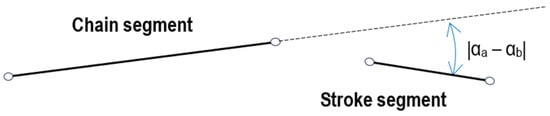
Figure 9. Different orientation between chain and dash.

The algorithm checks for orientation matching between stroke[i] and the chain segment.

For valid orientations, their merit (meritAngle) is calculated as a ramp function that equals 1 for exactly the same orientation, while it equals 0 for differences in orientation greater than the ThresholdAngle (Figure 10).

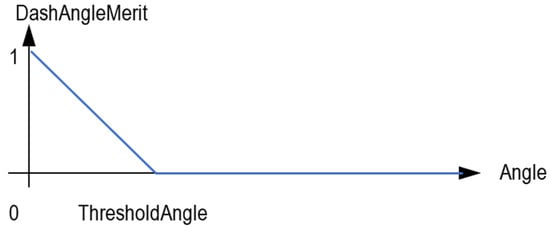
Figure 10. Orientation merit ramp function.

The offset value is determined as a combination of two factors. For very close lines, the gap line connecting their ends may be far from collinear. Alternatively, for more distant lines, the gap line discriminates poorly, while the step is the parameter that best measures the gap. We assume that when segments are closer to each other, the same step is perceived as more likely intentional. Hence, we measure both the angles and the step, as depicted in Figure 11:

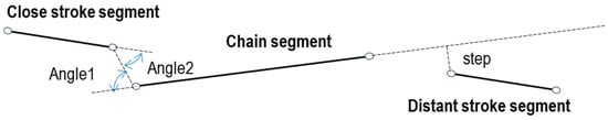
Figure 11. Offset measurement for close and distant dashes.

Angles are measured by simply selecting the greater one, and comparing against the threshold as described in Algorithm 5:

Algorithm 5: Angle measurement

1: if (max(Angle1, Angle2) > ThresholdAngle[i]) then 2: stroke[i] is discarded 3: end if;

The algorithm discards stroke[i] if the maximum angle exceeds the threshold.

For valid orientations, their merit (meritOffsetAngle) is calculated by the ramp function described in Figure 10.

To measure the step, the following calculations are performed. First, the maximum allowable step is calculated as a percentage (specified by ThresholdStep[i] in Equation (7)) of the length of the shortest segment (selected between stroke[i] and the chain).

$$OffsetStep\left[i\right]=Min\left(\left|stroke\left[i\right]\right|, \left|chain\right|\right)·ThresholdStep\left[i\right]$$

(7)

Second, the two distances of the tips that delimit the gap (A1 and B0 in the example of Figure 12) to the line defined by the other segment are calculated. The greater distance is selected as the “step” and compared to the offset (Algorithm 6).

Algorithm 6: Step comparison

if (step= max(dA1, dB0) > OffsetStep[i]) then discard stroke[i] end if;

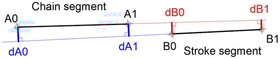
Figure 12. Distances from each tip to the line defined by the other segment.

The algorithm compares the maximum distance between the tips of the gap to the offset step.

For the valid steps, their merit (meritOffsetStep) is calculated as a ramp function that equals 1 for a null step, and 0 for greater than OffsetStep[i] (Figure 13).

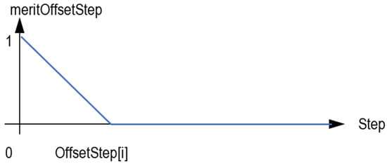
Figure 13. Step merit ramp function.

The merit of the whole offset (meritOffset) is calculated by balancing both meritOffsetAngle and meritOffsetStep, as follows:

$$meritOffset=\frac{meritOffsetAngle+meritOffsetStep}{2}$$

(8)

We note that both meritOffsetAngle and meritOffsetStep must not be null to obtain the candidate dash accepted as such.

MeritDash is finally calculated for each candidate dash, thus allowing the candidate dash with the highest merit to be added to the chain:

$$meritDash=\left[meritGap·DashBalanceGapAngle+meritAngle·\left(1-DashBalanceStepAngle\right)\right]·meritOffset$$

(9)

where DashBalanceStepAngle is an adjustable parameter (default is 50%).

4.4. Output Stroke Clustering

Upon completing the detection of a dashed stroke, the sketch undergoes an update to consolidate dashes. For each chain of dashed strokes, the process is described as follows:

• Create a chained stroke encompassing all the dashes of the chain.
• Save the chained stroke by replacing the first original dash.
• Remove the remaining dashes of the chain.

The chained stroke is created by linking the start point, midpoint, and endpoint of each dash. The endpoint of each dash is connected to the start point of the consecutive dash (Figure 14). A flag indicating whether each dash follows the same or the inverse direction of the chain is calculated in advance. Thus, the algorithm swaps the first and last points for reversed dashes (like the middle dash shown in Figure 14).

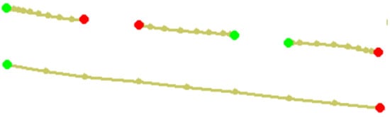
Figure 14. Chained stroke.

The output of our algorithm is the updated sketch, where dashes are removed and chained strokes are added (including their fitting parameters: coordinates of tips, length, and orientation).

5. Tuning Parameters

As said in the previous section, the algorithm requires the user to define several tuning parameters beforehand. These parameters are used to adapt the algorithm’s behavior to the characteristics of the sketch (sketching quality, stroke line style, etc.) and contribute to enhancing the algorithm’s overall efficiency. The choice of parameters along with the arguments to support the values assigned to them are explained based on the perceptual principles like the principle of continuity of the Gestalt law, combined with our own experience.

Table 1 summarizes the tuning parameters used in the decision-making rules defined in the previous section. They are grouped by their goals. The third column includes the suggested default values based on our experience. The implications of relaxing or restricting these values are also detailed in the table.

Table 1. User-adjustable tuning parameters.

Goal	Parameter	Default Value	If Increased	If Decreased
Exclude implausible dashes	DashSizeMax	50%	Computational time would be lost, as implausible dashes should be parsed.	Some dashed lines could be incomplete, as legitimate dashes should be labeled as non-candidate dashes.
	IsolatedTipThreshold	25%	Even very distant tips could be incorrectly labeled as sharing a vertex with the current stroke, which would be incorrectly labelled as non-candidate dash.	Edges sharing non-perfectly sketched vertices could be incorrectly labeled as candidate dashes (Figure 6).
Detect similar dashes	DashSizeShortRange	5 (times shorter than average length)	Excessively short strokes, intended to represent dots, could be accepted as valid dashes (Figure 7).	Only fairly regular dashed lines with dashes close to the average length would be accepted.
	DashSizeLongRange	2.5 (times longer than average length)	Excessively long strokes could be accepted as valid dashes, thus incorrectly connecting solid lines to dashed lines.	Only regular dashed lines with dashes close to the average length would be accepted.
Detect chains	DashGapShortRange	10 (times shorter than average length)	Excessively short gaps could be accepted. Consecutive lines could be incorrectly converted into dashed lines.	Only regular dashed lines with gaps close to the average length would be accepted.
	DashGapLongRange	2 (times longer than average length)	Excessively long gaps could be accepted. Consecutive dashed lines could be merged.	Only regular dashed lines with gaps close to the average length would be accepted.
	MaxDashAngle	20°	Dashed arcs would be detected, while closely parallel dashed straight strokes could become incorrectly merged.	Small failures in alignment of dashes could result in false negatives.
	MaxDashOffset	15%	More irregular dashed lines would be detected, at the cost of producing false positives, by grouping dashes of parallel dashed lines.	Even small irregularities would prevent actual dashed lines from being detected.
	IncreasedDashTolerances	50%	Tolerances would be further increased for short dashes.	Tolerances for short dashes would be very similar to those for long dashes.
	DashBalanceStepAngle	50%	Step would be more critical than orientation of the gap line. This would be better for sparse dashes.	Orientation of the gap line would be more critical than step. This would be better for dense dashes.
Check straightness	MaxNonStraightDashes	40%	Low-quality dashes would be accepted as straight.	Dashed lines would only be made of clearly straight dashes.
	LineTolMin	5%	Low-quality dashes could be incorrectly labeled as meritorious straight lines.	High-quality dashes could be incorrectly labeled as non-straight lines.
	LineTolMax	15%	Low-quality dashes could be incorrectly labeled as acceptable straight lines.	Acceptable-quality dashes could be incorrectly labeled as non-straight lines.
	LineSmoothPenalty	0.1%	A larger number of irregular dashes would be accepted as straight.	Only nearly perfect strokes would be fitted as straight lines.
	DashMinMeritLine	0.25 (over 1)	Could result in false negatives. Only very straight dashes would be labeled as straight.	Could result in false positives, as clearly non-straight dashes could be labeled as straight.

The filter IsolatedTipThreshold is critical to prevent false positives. Failure in removing non-isolated strokes as candidate dashes (resulting from reducing the parameter) can result in false-positive dashed strokes such as those shown in Figure 15.

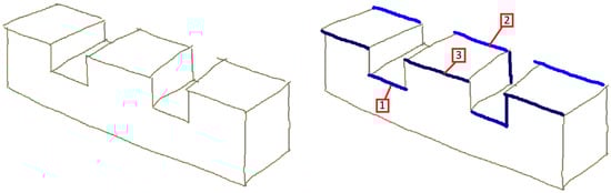
Figure 15. False dashed strokes grouped by color. Each group is numbered to differentiate between them.

The recommended value of the filter DashSizeShortRange (which controls DashLengthMin) may result in false positives (as dash–dot lines are classified as dashed lines) by ignoring the interspersed dots or short dashes (Figure 16). The detection of dash–dot lines in advance would solve this problem. The removal of this filter would naively allow for the detection of dash–dot lines, but short dashes should be parsed as dots (thus preventing checking its orientation, which is prone to be irrelevant).

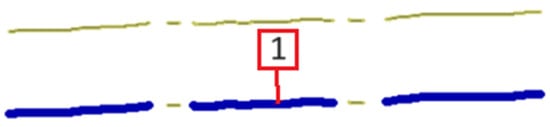
Figure 16. Dash–dot line parsed as a dashed line.

Even dashes that are too close are clearly perceived as such when looking at an isolated dashed line (Figure 17), but accepting very small gaps could result in chaining crossing dashed lines.

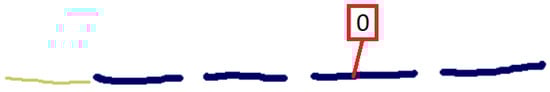
Figure 17. Excessively short gap.

The filters DashGapShortRange and DashGapLongRange act in tandem to delimit the range of admissible lengths of the intervals between consecutive dashes. The proposed values (10, 2) are a compromise solution to detect both lines with very close dashes (see the condensed dashed stroke in the upper side of Figure 18), and those with more dispersed dashes (see the scattered dashed stroke in the lower side of Figure 18). For example, decreasing DashGapShortRange results in failures in detecting condensed dashed strokes: a value of 4 (instead of 10) results in incorrectly labeling one single dashed stroke as two overlapped dashed strokes with alternating dashes. To further increase the effectiveness of the algorithm, this pair of parameters should be tuned differently to detect condensed dashes (20, 1) and scattered dashes (4, 4).

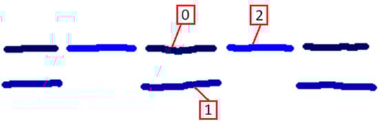
Figure 18. Condensed dashed stroke, incorrectly parsed as two overlapped dashed strokes (top), and scattered dashed stroke (bottom). Each dashed stroke group is numbered for clarity.

The filter MaxDashOffset is highly sensitive, as a small gap variation may prevent poorly drawn dashed strokes from being accurately chained (Figure 19). Further increasing its value, however, would result in the incorrect chaining of dashes that belong to closely parallel dashed strokes.

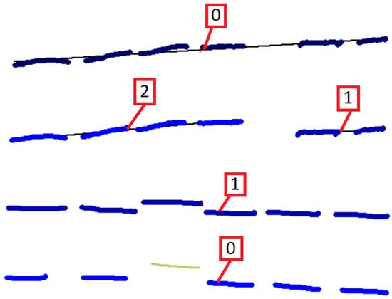
Figure 19. Upper dashed stroke is below offset threshold, while lower dashed stroke is above.

Additionally, relaxing MaxDashAngle and MaxDashOffset may result in false negatives for close parallel dashed lines that may be incorrectly chained with some swapped dashes (Figure 20).

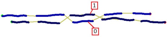
Figure 20. Swapped dashes in parallel dashed strokes.

6. Evaluation

Table 2 presents a collection of representative examples on which the algorithm has been tested. The left column depicts hand-drawn sketches with diverse arrangements of dashed lines and varying sketch qualities. The right column illustrates the outcome of the algorithm, reflecting the results of the vectorization process. In all cases, the results obtained are accurate and coherent. It is important to note that a significant factor that influences a successful outcome is the quality of the sketch’s strokes. Example 6A and 6B show that the algorithm generally avoids false positives.

Table 2. Examples of input freehand sketches and the results after the vectorization process.

	A		B
1
2
3
4
5
6

It is important to consider the current limitations of the algorithm, as they represent new opportunities for improvement and areas for future work. Naturally, these improvements go beyond the fact that the algorithm requires many adjustable parameters to accommodate different drawing styles for the dashed lines, and different contexts in which those lines are used. A future improvement should focus on distinguishing between straight dashed lines and dashed arcs (Figure 21), which could be achieved by replacing the collinearity constraint with a constant or “smooth” and “similar” rotation.

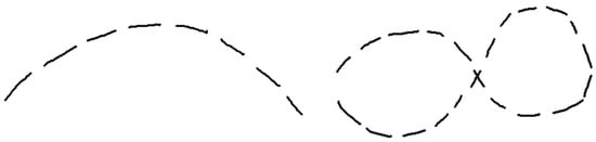
Figure 21. Examples of curved dashed strokes.

Finally, the weakest point of this method is the dependence on the sequence. To eliminate this dependence in which the strokes are drawn, the algorithm reorders the dashes by size. It is assumed that smaller strokes are more likely to be dashes of a dashed line, so they are reordered from smallest to largest. However, the primary characteristic of the method is that it seeks to chain successive strokes. Therefore, it is very sensitive to the chaining sequence. It is particularly sensitive to the stroke that is selected first. In the upper dashed line in Figure 22, the shortest stroke is the one tine of the fork shape (stroke 1). The behavior of the algorithm is different from that of the lower dashed stroke, which is an exact copy of the first line in which a shorter stroke has been added to the handle of the fork (stroke 11), causing the algorithm to start chaining at said farthest end. In the upper line, stroke 3 is chained, as it is close and reasonably aligned with stroke 1. In the lower line, stroke 9 is not very close to the chain as stroke 6 is, but it is much more aligned with the chain. To resolve these types of situations, the algorithm searches for forks, and then starts chaining from the handle side.

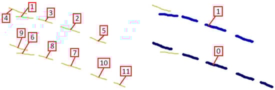
Figure 22. Chaining from the intersection, vs. chaining from the extreme.

7. Conclusions

Although it may seem trivial, the development of an algorithm capable of detecting hand-drawn dashed lines addresses an unsolved problem in the field of industrial product design. This paper highlights the importance of such an algorithm, particularly in scenarios where designers must resort to drawing continuous lines and subsequently manually editing them into dashed lines. Our proposed algorithm represents a significant step towards improving user experience by allowing applications to accurately interpret dashed lines. However, it is worth noting that our current solution is partial, as it does not yet extend to detecting other types of dashed lines, such as dot or dash–dot patterns.

To further highlight the novelty or complexity of the approach, we must remember that fixing dashed lines that are outlined with a ruler and compass is relatively straightforward. Simple algorithmic approaches based on geometric principles may work reasonably well. The problem becomes much more challenging when lines are hand-drawn. In this scenario, simple algorithms lack the human capability to perceive, balance, and make choices about small imperfections. Collinear dashes become “nearly” collinear, to cite but one example.

The main contribution of this paper is the idea of “following the path” to find preceding or following dashes until completing the chain of dashes. The approach works with local information while favoring the formulation of the perceptual principles as cues and requisites. These cues are then managed as constraints, which are tuned by different parameters, with values supported by perceptual principles combined with our own experience.

Finally, the algorithm, which was intended as a proof-of-concept, was validated with a wide and varied set of examples. We concluded that, with properly balanced parameters, the level of false negatives is acceptable, and the level of false positives is very small. These are good results, when put in the context of being one of the many stages that contribute to complete a complex vectorization and 3D reconstruction process. In these processes, false positives are difficult to detect and correct in later stages, whereas false negatives can be detected and “repaired” when global information comes into play in subsequent stages.

The use of expert systems remains worthy of exploring in future research. Yet, the main guidelines of the current approach—which mimics human perception—can be useful to shorten the training period, and focus on the most critical aspects of detecting these geometrically imperfect, yet fully perceivable, hand-drawn dashed lines.

References

- ISO 128-2:2020; Technical Product Documentation (TPD)—General Principles of Representation—Part 2: Basic Conventions for Lines. ISO: Geneva, Switzerland, 2020.
- Veisz, D.; Namouz, E.Z.; Joshi, S.; Summers, J.D. Computer-aided design versus sketching: An exploratory case study. AI EDAM 2012, 26, 317–335. [Google Scholar] [CrossRef]
- Camba, J.D.; Pedro Company; Naya, F. Sketch-Based Modeling in Mechanical Engineering Design: Current Status and Opportunities. Comput. Aided Des. 2022, 150, 103283. [Google Scholar] [CrossRef]
- Hähnlein, F. Binary Optimization for the Analysis and Synthesis of Concept Sketches. Ph.D. Thesis, d’Université Côte d’Azur, Inria Sophia Antipolis-Méditerannée, Nice, France, 2022. [Google Scholar]
- Agrawala, M.; Li, W.; Berthouzoz, F. Design Principles for Visual Communication. Commun. ACM 2011, 54, 60–69. [Google Scholar] [CrossRef]
- Pedro Company; Plumed, R.; Varley, P.A.; Camba, J.D. Algorithmic perception of vertices in sketched drawings of polyhedral shapes. ACM Trans. Appl. Percept. (TAP) 2019, 16, 18. [Google Scholar] [CrossRef]
- Bonnici, A.; Camilleri, K. An evolutionary approach to determining hidden lines from a natural sketch. In Proceedings of the IEEE Symposium on Visual Languages and Human-Centric Computing, Cambridge, UK, 4–8 September 2016. [Google Scholar]
- Varley, P.A.C. Automatic Creation of Boundary-Representation Models from Single Line Drawings. Ph.D. Thesis, Department of Computer Science, Cardiff University, Cardiff, UK, 2003. [Google Scholar]
- Varley, P.A.C.; Martin, R.R.; Suzuki, H. Frontal Geometry from Sketches of Engineering Objects: Is Line Labelling Necessary? Comput. Aided Des. 2005, 37, 1285–1307. [Google Scholar] [CrossRef]
- Kyratzi, S. Industrial-Product Concept Development: Geometric and Information Models for Interactive Design. Ph.D. Thesis, University of the Aegean, Lemnos, Greek, 2007. [Google Scholar]
- Kyratzi, S.; Sapidis, N. Extracting a polyhedron from a single-view sketch: Topological construction of a wireframe sketch with minimal hidden elements. Comput. Graph. 2009, 33, 270–279. [Google Scholar] [CrossRef]
- Kyratzi, S.; Azariadis, P. Geometric Definition of the Hidden Part of a Line Drawing in a Sketch-to-Solid Methodology. Comput. Aided Des. Appl. 2014, 12, 355–365. [Google Scholar] [CrossRef]
- Conesa, J. Reconstruccion Geometrica de Solidos Utilizando Tecnicas de Optimizacion. Ph.D. Thesis, Department of Structures and Construction, Polytechnic University of Cartagena, Cartagena, Spain, 2001. (In Spanish). [Google Scholar]
- Varley, P.A.C.; Pedro Company. A new algorithm for finding faces in wireframes. Comput. Aided Des. 2010, 42, 279–309. [Google Scholar] [CrossRef]
- Jorge, J.A.; Fonseca, M.J. A simple approach to recognize geometric shapes interactively. In Lecture Notes in Computer Science, Proceedings of the GREC’99, LNCS 1941; Springer: Berlin/Heidelberg, Germany, 2000; pp. 266–274. [Google Scholar]
- Lai, C.P.; Kasturi, R. Detection of dashed lines in engineering drawings and maps. In Proceedings of the First International Conference on Document Analysis and Recognition, Saint-Malo, France, 30 September–2 October 1991; pp. 507–515. [Google Scholar]
- Agam, G.; Luo, H.; Dinstein, I. Morphological approach for dashed lines detection. In Graphics Recognition Methods and Applications, Proceedings of the GREC’95, LNCS 1072; Kasturi, R., Tombre, K., Eds.; Springer: Berlin/Heidelberg, Germany, 1996. [Google Scholar] [CrossRef]
- Fu, L.; Kara, L.B. From engineering diagrams to engineering models: Visual recognition and applications. Comput. Aided Des. 2011, 43, 278–292. [Google Scholar] [CrossRef]
- Moon, Y.; Lee, J.; Mun, D.; Lim, S. Deep Learning-Based Method to Recognize Line Objects and Flow Arrows from Image-Format Piping and Instrumentation Diagrams for Digitization. Appl. Sci. 2021, 11, 10054. [Google Scholar] [CrossRef]
- Sang-Min, P.; Young-Gab, K. Visual language integration: A survey and open challenges. Comput. Sci. Rev. 2023, 48, 100548. [Google Scholar] [CrossRef]
- Plumed, R.; Pedro Company; Varley, P.A.C. A new approach for perceptually-based fitting strokes into straight segments. In Proceedings of the CEIG 2015, XXV Spanish Computer Graphics Conference, Benicàssim, Spain, 1–3 July 2015; pp. 81–89. [Google Scholar] [CrossRef]
- Pedro Company; Plumed, R.; Varley, P.A.C. A fast approach for perceptually-based fitting strokes into elliptical arcs. Vis. Comput. 2015, 31, 775–785. [Google Scholar] [CrossRef]
- Ku, D.C.; Qin, S.F.; Wright, D.K. Interpretation of Overtracing Freehand Sketching for Geometric Shapes. In Proceedings of the WSCG’2006, Plzen, Czech Republic, 30 January–3 February 2006; ISBN 80-86943-03-8. [Google Scholar]
- Bartolo, A.; Camilleri, K.P.; Fabri, S.G.; Borg, J.C.; Farrugia, P.J. Scribbles to vectors: Preparation of scribble drawings for CAD interpretation. In Sketch-Based Interfaces and Modeling 2007—ACM SIGGRAPH/Eurographics Symposium Proceedings; ACM: New York, NY, USA, 2007; pp. 123–130. [Google Scholar]
- Wang, S.; Qin, S.; Gao, M. Overtraced strokes to single line drawing: Preparation of sketch for 3D interpretation. In Proceedings of the 18th International Conference on Automation and Computing (ICAC), Loughborough, UK, 7–8 September 2012. [Google Scholar]
- Wang, S.; Qin, S.; Gao, M. New grouping and fitting methods for interactive overtraced sketches. Vis. Comput. 2014, 30, 285–297. [Google Scholar] [CrossRef]
- Wang, S.; Wang, S.; Li, Y.; Zhang, Q. Grouping of Multiple Overtraced Strokes in Interactive Freehand Sketches. In Proceedings of the 14th International Conference on Computer-Aided Design and Computer Graphics (CAD/Graphics), Xi’an, China, 26–28 August 2015; pp. 232–233. [Google Scholar] [CrossRef]
- Xiong, Y.; LaViola, J. A ShortStraw-Based Algorithm for Corner Finding in Sketch-Based Interfaces. Comput. Graph. 2010, 34, 513–527. [Google Scholar] [CrossRef]
Disclaimer/Publisher’s Note: The statements, opinions and data contained in all publications are solely those of the individual author(s) and contributor(s) and not of MDPI and/or the editor(s). MDPI and/or the editor(s) disclaim responsibility for any injury to people or property resulting from any ideas, methods, instructions or products referred to in the content. |
© 2024 by the authors. Licensee MDPI, Basel, Switzerland. This article is an open access article distributed under the terms and conditions of the Creative Commons Attribution (CC BY) license (https://creativecommons.org/licenses/by/4.0/).