Dynamics and Control of Satellite Formations Invariant under the Zonal Harmonic Perturbation

Abstract

A satellite formation operating in low-altitude orbits is subject to perturbations associated to the higher-order harmonics of the gravitational field, which cause a degradation of the formation configurations designed based on the unperturbed model of the Hill–Clohessy–Wiltshire equations. To compensate for these effects, periodic reconfiguration maneuvers are necessary, requiring the prior allocation of a propellant mass budget and, eventually, the use of resources from the ground segment, having a non-negligible impact on the complexity and cost of the mission. Using the Hamiltonian formalism and canonical transformations, a model is developed that allows designing configurations for formation flying invariant with respect to the zonal harmonic perturbation. $J_n$ invariant configurations can be characterized, selecting the drift rate (or boundedness condition) and the amplitude of the oscillations, based on four parameters which can be easily converted in position and velocity components for the satellites of the formation. From this model, a guidance strategy is developed to inject a satellite approaching another spacecraft into a bounded relative trajectory about it and the optimal time for the maneuver, minimizing the total $\mathrm{\Delta }V$, is identified. The effectiveness of the model and of the guidance strategy is verified on some scenarios of interest for formations operating in a sun-synchronous and a medium-inclination low Earth orbit and a medium-inclination lunar orbit.

1. Introduction

In the last decade, the number of proposed formation flying missions has increased significantly [1,2,3], led by the growing number of low-cost rideshare opportunities to low Earth orbits (LEO) with medium inclination (50–55 degrees) and to sun-synchronous orbits (SSO). Satellite formations operating in these orbits are affected by perturbations associated with the non-uniform Earth gravitational field [4,5], which depend on the position of the spacecraft and therefore have a different impact on each satellite of the formation [6,7]. Satellite formations designed using the traditional approach based on the Hill–Clohessy–Wiltshire (HCW) equations show an unstable behavior over time, characterized by marked variations in the amplitude of the in-plane and out-of-plane oscillations, and by the drift of the relative orbit center [8,9]. These effects have a dramatic impact on the performance of the formation, since the relative distance between the satellites can increase and exceed the operative range or decrease down to potential collision. In such a scenario, periodic reconfiguration maneuvers are required and they can eventually involve expensive coordination activity from the ground segment [10,11,12,13,14]. An effective alternative is to identify configurations which are stable with respect to the gravitational perturbations.

Several research works address the identification of satellite formations that are invariant under gravitational perturbations, most of them considering only the effects associated with the dominant J2 term. The first work on this topic is by Schaub and Alfriend, who derived two first-order conditions to design J2-invariant relative orbits, which can be applied on a large number of practical cases [15]. Schweighart and Sedwick developed a high-fidelity linearized model which takes into account the time-averaged effect of J2 [16], Kolemen, Kasdin, and Gurfil used the Hamiltonian formalism and the variation of parameters procedure to determine configurations stable under the effects of J2 [17]. Sabatini, Izzo, and Bevilacqua identified some values of the inclination corresponding to minimum drift orbits for the J2 perturbed case [18]. He, Armellin, and Xu developed a model to design bounded relative orbits in the full zonal problem, therefore including the $J_n$ terms up to the desired degree, based on the Taylor approximation of Poincaré maps and numerical refinement [19]. Ma et al. examined the same problem to determine invariant relative orbits (negligible drift and variation in the amplitude of the oscillations) using double-averaged Delaunay orbital elements [20].

In this work, a model providing a compact representation of invariant relative orbits for formation flying in the full zonal problem is introduced. Using the Hamiltonian formalism, canonical transformations allow absorbing the terms associated with the perturbation [21,22] and providing a new representation of the system dynamics in terms of three mutually orthogonal couples of state variables. It is proved that the relative orbit can be characterized in terms of four parameters, corresponding to the value of four state variables at a given time, with two of them defining the boundedness condition (or equivalently the drift rate) and the other two characterizing (independently) the amplitude of the in-plane and out-of-plane oscillations.

The model proposed here can be conveniently used to design bounded satellite formations stable under the full zonal harmonic perturbation. Furthermore, it allows developing a simple guidance strategy to inject a spacecraft approaching a target satellite into a stable bounded relative orbit. The effectiveness of the model and of the guidance strategy proposed are verified by means of numerical integration, using gravity field models including harmonic coefficients with high degree and order and real ephemerides.

The results are evaluated for satellite formations operating in some scenarios of interest: a SSO with altitude of 530 km, a circular LEO with medium inclination, and a circular lunar orbit with altitude of 4300 km and inclination of 40 degrees. These scenarios have been selected as they are of interest for some formation flying missions analyzed in recent years or under development, including ones in which the author was involved. In particular, it shall be noted that, beyond the popular SSO [1], medium-inclination LEO is attracting growing interest in recent years due to the increasing number of launches, led by the development of the Starlink constellation [23], and due to their suitability for Earth observation and remote sensing applications [24,25,26]. Finally, medium-inclination lunar orbits have emerged as a viable solution for lunar navigation systems [27,28,29].

2. Hamiltonian Formalism for Formation Flying under Zonal Harmonic Perturbation

The relative motion between two spacecraft $S{C}_1$ and $S{C}_2$ can be conveniently described using an orthogonal reference system ${\mathcal{F}}_r={\left[\begin{array}{ccc}\widehat{x}& \widehat{y}& \widehat{z}\end{array}\right]}^T$ centered in $S{C}_1$, named the chief satellite, with axes $\widehat{x}$ pointing from the center of the Earth to $S{C}_1$, $\widehat{z}$ parallel to the angular momentum of the chief orbit, and $\widehat{y}$ completing the orthogonal frame. The relative position and velocity of $S{C}_2$, named the deputy satellite, with respect to $S{C}_1$ are given by $\rho ={\left[\begin{array}{ccc}x& y& z\end{array}\right]}^T$ and $\dot{\rho }=\frac{d\rho }{dt}={\left[\begin{array}{ccc}{v}_x& v_y& v_z\end{array}\right]}^T$.

The dynamics of the two satellites evolve under the effects of the Earth gravitational potential, which can be modeled using spherical harmonics [4]:

$$V_i=-\frac{\mu }{r_i}\left[1-\sum _{n=2}^{\infty }\sum _{m=0}^n{\left(\frac{R_E}{r_i}\right)}^n{P}_{nm}(cos\varphi )(C_{nm}cosm\lambda +S_{nm}sinm\lambda )\right]$$

(1)

where μ = 3.986 × 10⁵ km³/s² and R_E = 6378 km are, respectively, the Earth gravitational parameter and equatorial radius, $r_i$ is the orbit radius of the i-th spacecraft, $P_{nm}$ are the Legendre associated functions of degree n and order m, $C_{nm}$ and $S_{nm}$ are the spherical harmonics coefficients, $\varphi$ is the geocentric co-latitude, and $\lambda$ is the longitude. To develop the model proposed in Section 3, Equation (1) is simplified considering only the zonal harmonic terms ($m=0$).

$$V_i=-\frac{\mu }{r_i}\left[1-\sum _{n=2}^{\infty }{J}_n{\left(\frac{R_E}{r_i}\right)}^n{P}_n(cos\varphi )\right]$$

(2)

It shall be noted that for satellite formations operating in Earth orbits, this approximation is acceptable, based on the fact that the secular perturbation associated with the zonal harmonic terms is larger by more than one order of magnitude than the periodic perturbations associated with the tesseral and sectorial harmonic ones ($m>0$) of the same degree [30]. Nevertheless, this is not a general case and, therefore, the model developed under this approximation is verified by means of numerical integration, discussed in Section 4, using orbital propagators which include all the harmonic coefficients.

The relative dynamics are expressed here using the Hamiltonian formalism in terms of the dimensionless state variables $\mathbf{q}$ and $\mathbf{p}$:

$$\left\{\begin{array}{c}\dot{\mathbf{q}}=\frac{\partial H}{\partial \mathbf{p}}\hfill \\ \dot{\mathbf{p}}=-\frac{\partial H}{\partial \mathbf{q}}\hfill \end{array}\right.$$

(3)

For the sake of compactness, the derivation of the model is presented in Appendix A and the expressions of the conjugate momenta and of the Hamiltonian function H are reported below:

$$\left\{\begin{array}{c}{p}_x=v_x-y+v_x^{\left(1\right)}\hfill \\ p_y=v_y+x+1+v_y^{\left(1\right)}\hfill \\ p_z=v_z+v_z^{\left(1\right)}\hfill \end{array}\right.$$

(4)

$$H=H^{\left(0\right)}\left(\mathbf{q},\mathbf{p}\right)+H^{\left(1\right)}\left(\mathbf{q},\mathbf{p},J_n\right)+H^{\left(2\right)}\left(\mathbf{q},\mathbf{p},J_n^2\right)$$

(5)

where

$$H^{\left(0\right)}=\frac{1}{2}{\left(p_x+y\right)}^2+\frac{1}{2}{\left(p_y-1-x\right)}^2+\frac{p_z^2}{2}-\frac{3}{2}{x}^2+\frac{z^2}{2}$$

(6)

$$H^{\left(1\right)}=-v_x^{\left(1\right)}{p}_x-v_y^{\left(1\right)}{p}_y-v_z^{\left(1\right)}{p}_z+K_{10}x+K_{20}y+K_{30}z$$

(7)

$$H^{\left(2\right)}=K_{11}{x}^2+K_{22}{y}^2+K_{33}{z}^2$$

(8)

The reader will notice that the expression of $H^{\left(0\right)}$ is equal to that of the Hamiltonian function for the unperturbed case, while $H^{\left(1\right)}$ and $H^{\left(2\right)}$ depend on, respectively, the parameters $J_n$ and $J_n^2$, collected in the coefficients $v_i^{\left(1\right)}$ and $K_{ij}$.

As detailed in Appendix A.2, the parameter $J_n$ is small (i.e., $J_n<<1$). It is known that the terms of a Hamiltonian function depending on small parameters can be absorbed by a canonical change in coordinates, which preserves the form of the Hamilton Equation (3) [21]. This technique is applied in Section 3 to absorb $H^{\left(1\right)}$ and rearrange the Hamiltonian function as the sum of $H^{\left(0\right)}$ plus negligible higher order terms [31].

3. Characterization of Invariant Relative Orbits

In this section, canonical transformations are introduced to develop a model providing a compact characterization of relative orbits which are invariant with respect to the zonal harmonic perturbation, modeled using the $J_n$ terms up to the desired degree. The first set of canonical transformations allows absorbing the effects associated with the perturbation, resulting in a form of H equivalent to $H_0$. The last transformation allows expressing the Hamiltonian function as a sum of three terms, representing the nature of the relative orbit (bounded or unbounded) and the amplitude of the in-plane and out-of-plane oscillations, respectively.

3.1. Canonical Transformations Absorbing the Zonal Harmonic Perturbation

The canonical transformations ${\mathcal{T}}_i:\left(\mathbf{q},\mathbf{p}\right)\to \left(\mathbf{Q},\mathbf{P}\right)$ are developed to rearrange the Hamiltonian function from the form given by Equation (5) to the following one:

$$\tilde{H}=H^{\left(0\right)}\left(\mathbf{Q},\mathbf{P}\right)+o\left(J_n^k\right)$$

(9)

where $o\left(J_n^2\right)$ represents the negligible higher-order terms associated with the zonal harmonic perturbation.

As shown by Equations (6)–(8), the dynamics onto the $[\widehat{x},\widehat{y}]$ plane are not coupled to the one along the $\widehat{z}$ direction, so the canonical transformations for the in-plane ($x,y,p_x,p_y$) and the out-of-plane ($z,p_z$) state variables can be developed separately. The perturbation terms in the out-of-plane dynamics can be absorbed by introducing a type-3 generating function $S_3\left(z,P_z\right)$ such that

$$\left\{\begin{array}{c}{p}_z=\frac{\partial S_3}{\partial z}\hfill \\ Q_z=\frac{\partial S_3}{\partial P_z}\hfill \end{array}\right.$$

(10)

Setting $S_z=\frac{\partial S_3}{\partial z}$, introducing Equation (11) into Equations (6)–(8), and isolating the out-of-plane terms results in

$${\tilde{H}}_z=\frac{S_z^2}{2}+\frac{1+K_{33}^2}{2}{z}^2-v_z^{\left(1\right)}{S}_z+K_{30}z$$

(11)

The desired transformation $S_3$ can be found after determining the expression of $S_z$ such that

$${\tilde{H}}_z=\frac{P_z^2}{2}+\frac{1+K_{33}^2}{2}{z}^2$$

(12)

Equations (11)–(12) can be solved by quadrature

$$S_z^2-2v_z^{\left(1\right)}{S}_z+2K_{30}z-P_z^2=0\to$$

$$\to S_z=v_z^{\left(1\right)}\pm \sqrt{v_z^{{\left(1\right)}^2}-\left(2K_{30}z-P_z^2\right)}$$

(13)

and Equation (13) can be integrated to produce

$$S_3\left(z\right)=v_z^{\left(1\right)}z\mp \frac{{\left[v_z^{{\left(1\right)}^2}-2K_{30}z+P_z^2\right]}^{\frac{3}{2}}}{3K_{30}}+C_3$$

(14)

where $C_3$ is the (inessential) constant of integration. Introducing Equation (13) into Equation (11) results in the following canonical changes in coordinates:

$${\mathcal{T}}_3:z=\frac{\left[P_z^2+v_z^{{\left(1\right)}^2}-K_{30}^2\frac{Q_z^2}{P_z^2}\right]}{2K_{30}}$$

(15)

$${\mathcal{T}}_6:p_z=v_z^{\left(1\right)}\pm K_{30}\frac{Q_z}{P_z}$$

(16)

The in-plane terms are too complex to be processed and the use of normal forms is preferred. As proved in Appendix B, using the type-3 generating function $S\left(x,y,P_x,P_y\right)$ results in the following canonical change in coordinates:

$${\mathcal{T}}_1:x=Q_x-g_1$$

(17)

$${\mathcal{T}}_2:y=Q_y-g_2$$

(18)

$${\mathcal{T}}_3:p_x=P_x+f_1$$

(19)

$${\mathcal{T}}_4:p_y=P_y+f_2$$

(20)

where

$$\left\{\begin{array}{c}{f}_1=\frac{v_x^{\left(1\right)}\left(1+2K_{22}\right)+K_{20}}{2K_{22}}\hfill \\ f_2=\frac{K_{10}}{2\left(1-K_{11}\right)}+\frac{v_y^{\left(1\right)}\left(3-2k_{11}\right)}{2\left(1-K_{11}\right)}\hfill \\ g_1=v_y^{\left(1\right)}-f_2\hfill \\ g_2=f_1-v_x^{\left(1\right)}\hfill \end{array}\right.$$

(21)

The Hamiltonian function obtained after applying the ${\mathcal{T}}_i$ transformations is reported below

$$\tilde{H}=\frac{1}{2}{\left(P_x+Q_y\right)}^2+\frac{1}{2}{\left(P_y-1-Q_x\right)}^2+\left(K_{11}-\frac{3}{2}\right)Q_x^2+K_{22}{Q}_y^2+\frac{P_z^2}{2}+\frac{1+K_{33}^2}{2}{Q}_z^2$$

(22)

The reader can verify that the Hamilton Equation (3) obtained using $\tilde{H}$ correspond to the following set of second-order ordinary differential equations:

$$\left\{\begin{array}{c}{\ddot{Q}}_x=\left(2K_{11}-3\right)Q_x+2{\dot{Q}}_y\hfill \\ {\ddot{Q}}_y=-2{\dot{Q}}_x-2K_{22}{Q}_y\hfill \\ {\ddot{Q}}_z=-\left(1+K_{33}^2\right)Q_z\hfill \end{array}\right.$$

(23)

As declared at the beginning of this section, Equation (23) is equivalent to the HCW equations except for the negligible terms $K_{ii}$.

3.2. Siegel–Moser Canonical Transformation

The Hamilton Equation (3) obtained from $\tilde{H}$ corresponds to the following linear dynamical system:

$$\left[\begin{array}{c}\dot{\mathbf{Q}}\\ \dot{\mathbf{P}}\end{array}\right]=A\left[\begin{array}{c}\mathbf{Q}\\ \mathbf{P}\end{array}\right]$$

(24)

where

$$A=\left[\begin{array}{cccccc}0& 1& 0& 1& 0& 0\\ -1& 0& 0& 0& 1& 0\\ 0& 0& 0& 0& 0& 1\\ 2\left(1-K_{11}\right)& 0& 0& 0& 1& 0\\ 0& -1-2K_{22}& 0& -1& 0& 0\\ 0& 0& -1-2K_{33}& 0& 0& 0\end{array}\right]$$

(25)

Examining Equation (23), it is possible to state that the system admits an equilibrium point ${\mathbf{x}}^{★}={\left[\begin{array}{cc}\mathbf{Q}=\mathbf{0}& \mathbf{P}=\mathbf{0}\end{array}\right]}^T$, with one pair of real $(\pm \alpha )$ and two pairs of imaginary $(\pm i{\beta }_1,\pm i{\beta }_2)$ eigenvalues, corresponding to an equilibrium of the saddle–center–center type.

According to the Morse–Palais lemma, in the neighborhood of ${\mathbf{x}}^{★}$, the Hamiltonian function can be rearranged as the sum of three quadratic terms: one hyperbola (saddle) and two ellipses (centers). A transformation ${\mathcal{T}}_7:\left(\mathbf{Q},\mathbf{P}\right)\in \mathbb{R}\to \left(\mathbf{w},\mathbf{z}\right)\in \mathbb{C}$ is developed here that produces the above-mentioned form, diagonalizes A, and is symplectic (i.e., ${\mathcal{T}}_7$ is canonical) [32].

Indicating with $\mathrm{\Lambda }=diag\left(\alpha ,-\alpha ,j{\beta }_1,-j{\beta }_1,j{\beta }_2,-j{\beta }_2\right)$ the diagonal matrix of eigenvalues and with ${\mathbf{T}}_{\mathrm{\Lambda }}$ the matrix whose columns are the corresponding eigenvectors, the following permutation is introduced:

$$P=\left(\begin{array}{cccccc}1& 2& 3& 4& 5& 6\\ 1& 4& 2& 5& 3& 6\end{array}\right)$$

to obtain the Siegel–Moser form

$$\mathbf{T}=P\left({\mathbf{T}}_{\mathrm{\Lambda }}\right)=diag\left(\alpha ,j{\beta }_1,j{\beta }_2,-\alpha ,-j{\beta }_1,-j{\beta }_2\right)$$

(26)

For the transformation ${\mathcal{T}}_7$ to be canonical, $\mathbf{T}$ shall be transformed into a symplectic form $\mathbf{S}$. A matrix $\mathbf{Q}$ is introduced such that

$$\mathbf{S}=\mathbf{T}{\mathbf{Q}}^{-1}$$

(27)

having selected

$$\mathbf{Q}=\left[\begin{array}{cc}{\mathbf{B}}_1& \mathbf{0}\\ \mathbf{0}& \mathbf{I}\end{array}\right]$$

$$\mathbf{J}=\left[\begin{array}{cc}\mathbf{0}& \mathbf{I}\\ -\mathbf{I}& \mathbf{0}\end{array}\right]$$

$$\mathbf{B}={\left({\mathbf{J}}^{-1}{\mathbf{T}}^T\mathbf{J}\right)}^{-1}$$

where $\mathbf{I}$ is a $3\times 3$ identity matrix and ${\mathbf{B}}_1$ is the $3\times 3$ matrix corresponding to the first three rows and columns of $\mathbf{B}$. Finally, to verify that reality condition on the state variables $\left(\mathbf{Q},\mathbf{P}\right)$, matrix $\mathbf{S}$ shall be post-multiplied by

$$\mathbf{R}=diag\left(1,k_1,k_2,1,1/k_1,1/k_2\right)$$

where $k_1={\mathbf{s}}_{\mathbf{2}}^T{\mathbf{s}}_{\mathbf{5}}$, $k_2={\mathbf{s}}_{\mathbf{3}}^T{\mathbf{s}}_{\mathbf{6}}$, and ${\mathbf{s}}_i$ indicate the i-th column of $\mathbf{S}$.

We collect all the results of the transformations above in the following matrix:

$${\mathbf{T}}_N=P\left({\mathbf{T}}_{\mathrm{\Lambda }}\right){\mathbf{Q}}^{-1}\mathbf{R}$$

(28)

which produces

$${\mathcal{T}}_7:=\left[\begin{array}{c}\mathbf{Q}\\ \mathbf{P}\end{array}\right]={\mathbf{T}}_N\left[\begin{array}{c}\mathbf{w}\\ \mathbf{z}\end{array}\right]$$

(29)

$${\mathbf{T}}_N=\left[\begin{array}{cccccc}2c_1& c_1& 0& -2c_2& j{c}_1& 0\\ c_3& 2j{c}_1& 0& -c_3& 2c_1& 0\\ 0& 0& -c_1& 0& 0& -j{c}_1\\ -c_3& -j{c}_1& 0& c_1& -c_1& 0\\ -c_1& -c_1& 0& c_2& -j{c}_1& 0\\ 0& 0& -j{c}_1& 0& 0& -c_1\end{array}\right]$$

(30)

where the value of the coefficients $c_i\in {\mathbb{R}}^{+}$ of ${\mathbf{T}}_N$ can be obtained from Equation (28) and depends on that of the coefficients $K_{ij}$. From Equation (30), the reader can verify the following properties:

• the transformed variables $w_1$, $w_2$, $z_1$, and $z_2$ depend only on the in-plane components $Q_1$, $Q_2$, $P_1$, and $P_2$;
• the transformed variables $w_3$ and $z_3$ depend only on the out-of-plane components $Q_3$ and $P_3$;
• the imaginary part of $w_1$ and $z_1$ is null: $\Im (w_1,z_1)=0$;
• $z_i=-j\overline{w_i},i=2,3$.

In fact, the last property implies that $|w_2|=|z_2|$ and $|w_3|=|z_3|$, a condition that, as seen in the following section, allows the parametric characterization of relative trajectories in terms of only four parameters.

3.3. Characterization of $J_n$-Invariant Relative Trajectories

The transformation ${\mathcal{T}}_7$ produces the following form of the Hamiltonian function:

$$\widehat{H}=\alpha w_1{z}_1+\frac{{\beta }_1}{2}\left(w_2^2+z_2^2\right)+\frac{{\beta }_2}{2}\left(w_3^2+z_3^2\right)$$

(31)

The use of Hamilton Equation (3) shows that the dynamics on the three planes $\left(w_i,z_i\right)$ are not coupled and, because the Hamiltonian function is constant (see Appendix A), the three terms of Equation (31) are also constant.

The trajectories associated with the first term, and thus associated with the saddle type of equilibrium, are hyperbolas of equations

$$\left\{\begin{array}{c}{w}_1\left(t\right)=w_1\left(t_0\right)e^{\alpha t}\hfill \\ z_1\left(t\right)=z_1\left(t_0\right)e^{-\alpha t}\hfill \end{array}\right.$$

(32)

where $t_0$ indicates the value of the state variables at a specific time. Equation (32) is associated with trajectories that can diverge from $(z_1(t_0)=0)$, converge to $(w_1(t_0)=0)$, or oscillate indefinitely in time $(w_1(t_0)=z_1(t_0)=0)$ in the neighborhood of ${\mathbf{x}}^{★}$. In fact, the condition $w_1(t_0)=z_1(t_0)=0$ characterizes relative trajectories which are stably bounded (do not drift in time) also in the presence of the zonal harmonic perturbation.

Before validating the results through numerical integration, presented in Section 4, a preliminary proof of the model consists in verifying that it produces the well-known boundedness conditions for the unperturbed case, which can be derived from the HCW equations [11]

$$\left\{\begin{array}{c}{v}_y=-2x\hfill \\ v_x=\frac{y}{2}\hfill \end{array}\right.$$

(33)

This can be easily done by setting to zero the $K_{ii}$ terms in Equation (25), applying the Siegel–Moser transformation defined in Section 3.2 and making the condition $w_1=z_1=0$ explicit:

$$\left\{\begin{array}{c}x+p_y=1\hfill \\ y+p_x=0\hfill \end{array}\right.$$

(34)

Introducing the expressions of $p_x$ and $p_y$ from Equation (4) shows that two sets of Equations (33)–(34) are equal.

The last two terms of Equation (31) are harmonic oscillators associated with the center types of equilibrium. Recalling the properties in Section 3.2, it is possible to conclude that the amplitude of the in-plane oscillations is proportional to $|w_2|$ and, equivalently, that of the out-of-plane oscillations is proportional to $|w_3|$ [33].

It is worth summarizing here the main results obtained in Section 3:

• Applying the canonical transformations ${\mathcal{T}}_1$–${\mathcal{T}}_6$, the dynamics equations of relative motion in the full zonal problem are converted to a form equivalent to that of the unperturbed case plus negligible second-order terms. Trajectories designed in this framework are invariant with respect to the effects of the zonal harmonic perturbation.
• A last canonical transformation ${\mathcal{T}}_7$ produces a simplified representation of the dynamics, which can provide a compact characterization of invariant relative trajectories.
• Bounded relative trajectories evolving around ${\mathbf{x}}^{★}$ (i.e., the chief satellite) are quasiperiodic orbits characterized by $w_1\left(t_0\right)=z_1\left(t_0\right)=0$.
• The amplitude of the in-plane oscillations is proportional to $|w_2|$ (or equivalently $|z_2|$).
• The amplitude of the out-of-plane oscillations is proportional to $|w_3|$ (or equivalently $|z_3|$).

3.4. A Guidance Strategy for the Injection into a Bounded Orbit

The model defined in the previous section allows us to derive a simple guidance strategy to transfer a deputy satellite moving along a relative drift trajectory into a bounded orbit about the chief satellite. At a given time t, the deputy satellite is moving along a drift trajectory if $w_1\left(t\right)\ne 0$ and $z_1\left(t\right)\ne 0$. The satellite can be transferred into a bounded orbit after introducing $\delta w_1$ and $\delta z_1$ such that

$$\left\{\begin{array}{c}{w}_1\left(t\right)+\delta w_1=0\hfill \\ z_1\left(t\right)+\delta z_1=0\hfill \end{array}\right.$$

(35)

The conditions set by Equation (35) can be expressed in terms of relative position and velocity components and the instantaneous change in velocity required to establish the boundedness condition can be derived. First, the inverse of Equation (29) allows expressing $\delta w_1$ and $\delta z_1$ as a function of the instantaneous changes in $P_x$ and $P_y$, indicated as $\delta P_x$ and $\delta P_y$.

$$\left\{\begin{array}{c}\delta w_1=-2\frac{c_2}{c_2{c}_3-c_1^2}\delta P_x-\frac{c_1}{c_2{c}_3-c_1^2}\delta P_y=-w_1\left(t_0\right)\hfill \\ \delta z_1=-2\frac{c_1}{c_2{c}_3-c_1^2}\delta P_x-\frac{c_3}{c_2{c}_3-c_1^2}\delta P_y=-z_1\left(t_0\right)\hfill \end{array}\right.$$

(36)

Then Equation (36) can be solved in $\delta P_x$ and $\delta P_y$ and the $\mathrm{\Delta }v$ components can be determined, introducing Equation (4) in the solution.

$$\left\{\begin{array}{c}\delta v_x=\frac{c_3{w}_1\left(t_0\right)-c_1{z}_1\left(t_0\right)}{2}\hfill \\ \delta v_y=c_2{z}_1\left(t_0\right)-c_1{w}_1\left(t_0\right)\hfill \end{array}\right.$$

(37)

Finally, it is possible to determine the instant in which to operate the maneuver to minimize the total $\mathrm{\Delta }V=\sqrt{\delta v_x^2+\delta v_y^2}$. Recalling Equations (32), it is straightforward to determine that the time $t^{★}$ minimizing $\mathrm{\Delta }V$ is

$$\left\{\begin{array}{c}{t}^{★}=\frac{1}{4\alpha }log\frac{z_1^2\left(t_0\right)\left(\frac{c_1^2}{4}+c_2^2\right)}{w_1^2\left(t_0\right)\left(c_1^2+\frac{c_3^2}{4}\right)}\leftrightarrow z_1^2\left(t_0\right)\left(\frac{c_1^2}{4}+c_2^2\right)>w_1^2\left(t_0\right)\left(c_1^2+\frac{c_3^2}{4}\right)\hfill \\ t^{★}=t_0\leftrightarrow z_1^2\left(t_0\right)\left(\frac{c_1^2}{4}+c_2^2\right)<w_1^2\left(t_0\right)\left(c_1^2+\frac{c_3^2}{4}\right)\hfill \end{array}\right.$$

(38)

4. Numerical Study

The effectiveness of the model developed in Section 3 is verified by means of numerical integration, examining formations operating in some scenarios of interest: (a) an ELINT formation with the chief satellite in a SSO with altitude of 530 km, (b) a SAR formation with the chief satellite in a circular LEO with altitude of 530 km and inclination of 52 degrees, and (c) a formation at support of a lunar navigation system with the chief satellite on a circular lunar orbit with altitude of 4300 km and inclination of 40 degrees. Similarly, the guidance strategy is validated by applying it on a space reconnaissance satellite approaching a space object in a medium inclination LEO; the satellite is transferred into a bounded orbit about the object to be observed.

For all the cases, configurations invariant with respect to the zonal harmonic perturbation are identified in the Hamilton coordinates $\left(\mathbf{w},\mathbf{z}\right)$ and are then transformed to position and velocity coordinates $\left(\rho ,\dot{\rho }\right)$ in ${\mathcal{F}}_r$ by applying the inverse of canonical transformations ${\mathcal{T}}_1$–${\mathcal{T}}_7$, considering the combinations of the zonal coefficients $J_n$ selected as indicated in Appendix A.2.

The initial states selected in this way are then converted to dimensional form using the following factors for distance and time (see Appendix A.3):

$$\left\{\begin{array}{c}DU=\overline{a}\hfill \\ TU=1/n\hfill \end{array}\right.$$

(39)

where $\overline{a}$ and n are the chief orbit mean semimajor axis and angular velocity. The General Mission Analyisis Tool, developed by NASA’s Navigation and Ancillary Information Facility at the Jet Propulsion Laboratory, is used to propagate the initial states, using the DE405 ephemeris model [34]. The gravity field of the Earth is described by the JGM-2 model [35], including all the harmonic coefficients up to order and degree 70. For the gravity field of the Moon, the LP-165 model was used [36], including all the harmonic coefficients up to order and degree 165.

4.1. Formation in Sun-Synchronous Orbits

The stability of a satellite formation designed for SAR applications is evaluated. The orbit parameters of the chief satellite and the formation configuration, reported in Table 1 and Table 2, are selected according to the requirements for the implementation of SAR technology for the Micro-Satellite Clusters (MIRACLE)-II, a project by the European Defence Agency in which the author was involved for the mission analysis and platform design [26].

Table 1. SSO formation: orbit parameters chief satellite.

semimajor axis	$\overline{a}$	6919 km
eccentricity	e	0.002
inclination	i	97.79 deg
local time ascending node	-	11:00 am
epoch (UTC)	-	24 January 2023 12:00:00

Table 2. SSO formation: initial state of deputy satellite.

Hamiltonian Variables		Position/Velocity Components
$w_1$	0	x	9.7806 km
$w_2$	(1 + j) ·${10}^{-3}$	y	−19.5611 km
$w_3$	(1 + j) ·${10}^{-4}$	z	−0.9781 km
$z_1$	0	$v_x$	−14.2517 m/s
$z_2$	(−1 − j) · ${10}^{-3}$	$v_y$	−21.4989 m/s
$z_3$	(−1 − j) · ${10}^{-4}$	$v_z$	0 m/s

The relative orbit obtained from the integration of the initial conditions in Table 2 is represented in Figure 1, where the red line indicates the relative orbit for the first period and the black line is the complete trajectory over 30 days. The maximum and the minimum values of the three position coordinates for the first and the last orbit are reported in Table 3, showing that the amplitude of the in-plane oscillations increases by less than 0.05% and that of the out-of-plane oscillations decreases by 4%.

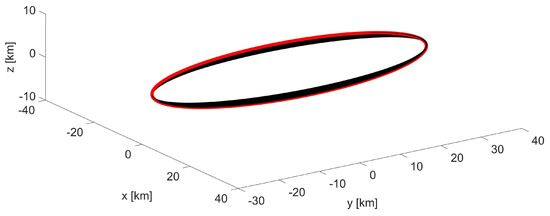
Figure 1. SSO formation: $J_n$-invariant bounded trajectory (black) in ${\mathcal{F}}_r$; the first orbit is plotted in red.

Table 3. SSO formation: maximum and minimum value of the position coordinates for the first and the last orbit.

First Orbit		Last Orbit
$x^{max}$	16.2582 km	$x^{max}$	16.2606 km
$x^{min}$	−16.2572 km	$x^{min}$	−16.2724 km
$y^{max}$	38.8642 km	$y^{max}$	38.9342 km
$y^{min}$	−26.1207 km	$y^{min}$	−26.0483 km
$z^{max}$	0.9807 km	$z^{max}$	0.9426 km
$z^{min}$	−0.9781 km	$z^{min}$	−0.9370 km

The results above are compared to the ones obtained from a trajectory designed based on the HCW Equation (23) having the same geometric properties. The effects of the perturbation on such a trajectory are clearly shown in Figure 2; neither the shape nor the center of rotation is preserved, as it is when using $J_n$-invariant initial states. The drift along the $\widehat{y}$ direction is shown in Figure 3 and evolves at an almost constant rate of 11 km/day. Figure 4 shows the time evolution of the z coordinate, representing the out-of-plane oscillations, which increase by 100% over 30 days, an effect 25 times higher than the one registered for the $J_n$-invariant case.

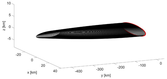
Figure 2. SSO formation: trajectory (black) in ${\mathcal{F}}_r$ resulting from non-invariant initial conditions; the first orbit is plotted in red.

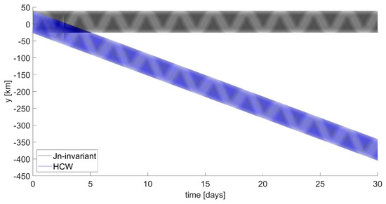
Figure 3. SSO formation: time behavior of y component.

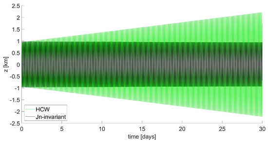
Figure 4. SSO formation: time behavior of z component.

4.2. Formation in Medium-Inclination Circular LEO

In this section, the stability of a satellite formation designed to perform ELINT is investigated. The orbit parameters of the chief satellite and the formation configuration are reported in Table 4 and Table 5 and result in the relative trajectory shown in Figure 5.

Table 4. Mid-inclination LEO formation: orbit parameters of chief satellite.

semimajor axis	$\overline{a}$	6919 km
eccentricity	e	0
inclination	i	52 deg
RAAN	$\mathrm{\Omega }$	0 deg
epoch (UTC)	-	24 January 2023 12:00:00

Table 5. Mid-inclination LEO formation: initial state of deputy satellite.

Hamiltonian Variables		Position/Velocity Components
$w_1$	0	x	9.7849 km
$w_2$	(1 + j) ·${10}^{-3}$	y	−19.5697 km
$w_3$	(1 + j) ·${10}^{-3}$	z	−9.7849 km
$z_1$	0	$v_x$	−7.5402 m/s
$z_2$	(−1 − j) · ${10}^{-3}$	$v_y$	−21.5257 m/s
$z_3$	(−1 − j) · ${10}^{-3}$	$v_z$	0.2797 m/s

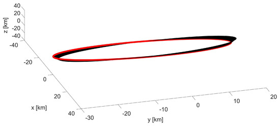
Figure 5. Mid-inclination LEO formation: $J_n$-invariant bounded trajectory (black) in ${\mathcal{F}}_r$; the first orbit is plotted in red.

As for the case in Section 4.1, the variations in the extreme values of the position coordinates for the first and the last orbit, collected in Table 6, are compared. The results indicate that both the in-plane and the out-of-plane oscillations decrease by a marginal 1.2% and 2.7%.

Table 6. Mid-inclination LEO formation: maximum and minimum value of the position coordinates for the first and the last orbit.

First Orbit		Last Orbit
$x^{max}$	11.9577 km	$x^{max}$	11.9611 km
$x^{min}$	−11.9724 km	$x^{min}$	−11.9790 km
$y^{max}$	18.0742 km	$y^{max}$	19.2724 km
$y^{min}$	−29.8000 km	$y^{min}$	−28.5862 km
$z^{max}$	9.5223 km	$z^{max}$	9.5223 km
$z^{min}$	−9.4888 km	$z^{min}$	−9.4888 km

The use of initial conditions determined based on the unperturbed model results in the trajectory represented in Figure 6, characterized by a high drift rate along the $\widehat{y}$ direction and rapid increase in the amplitude of the oscillations, which can be observed in detail in Figure 7 and Figure 8.

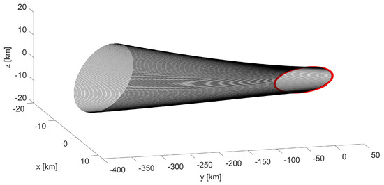
Figure 6. Mid-inclination LEO formation: trajectory (black) in ${\mathcal{F}}_r$ resulting from non-invariant initial conditions; the first orbit is plotted in red.

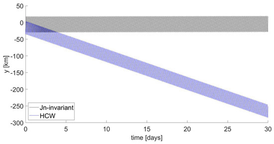
Figure 7. Mid-inclination LEO formation: time behavior of y component.

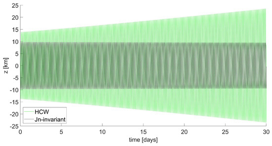
Figure 8. Mid-inclination LEO formation: time behavior of z component.

To further evaluate the effectiveness of the method developed in this research, relative trajectories computed from $J_n$-invariant initial states can be compared to the ones obtained integrating $J_2$-invariant initial states derived from the method proposed by Schaub and Alfriend, which is known to be effective especially for non-polar orbits. The orbit parameters of the chief satellite and the $J_2$-invariant initial state of the deputy satellite are the ones indicated in [15] and reported in Table 7 and Table 8.

Table 7. Mid-inclination eccentric LEO formation: orbit parameters of chief satellite.

semimajor axis	$\overline{a}$	7153 km
eccentricity	e	0.05
inclination	i	48 deg
RAAN	$\mathrm{\Omega }$	0 deg
argument of pericenter	$\omega$	30 deg
epoch (UTC)	-	24 January 2023 12:00:00

Table 8. Mid-inclination eccentric LEO formation: $J_2$-invariant initial state of deputy satellite.

x	−0.7156 km
y	0.2700 km
z	−0.3202 km
$v_x$	−0.0724 m/s
$v_y$	1.6135 m/s
$v_z$	0.3773 m/s

The $J_n$-invariant initial state is reported in Table 9. It shall be noted that the model proposed here is developed for satellites operating along orbits with null or negligible eccentricity (see Appendix A.1); therefore, its application on an elliptic orbit, like the one in Table 7, shall be carefully evaluated. Because the error introduced in Equations (A1)–(A5) for $e=0.05$ is of the order of ${10}^{-3}$ [37], an attempt was made to proceed further. The effectiveness of this approach can be verified from the results reported below, obtained by means of numerical integration.

Table 9. Mid-inclination eccentric LEO formation: $J_n$-invariant initial state of deputy satellite.

Hamiltonian Variables		Position/Velocity Components
$w_1$	0	x	−0.7156 km
$w_2$	(−1.069 + j0.072) ·${10}^{-4}$	y	0.2700 km
$w_3$	(−3.165 − j4.125) · ${10}^{-5}$	z	−0.3202 km
$z_1$	0	$v_x$	−0.0724 m/s
$z_2$	(−0.072 + j1.069) · ${10}^{-4}$	$v_y$	1.6142 m/s
$z_3$	(4.125 + j3.165) · ${10}^{-5}$	$v_z$	0.4173 m/s

The relative trajectories obtained integrating the two different initial states reported in Table 8 and Table 9 are computed as for the previous cases and represented in Figure 9. In particular, the figure represents the evolution of the two trajectories over 3 days from the initial epoch, showing that even in a short time, the use of $J_n$-invariant initial states can improve the boundedness condition established by selecting $J_2$-invariant initial states. The effect is particularly evident on the y component, whose time behavior is shown in Figure 10.

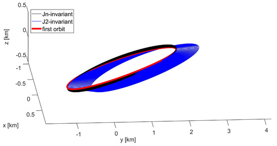
Figure 9. Mid-inclination eccentric LEO formation: trajectory in ${\mathcal{F}}_r$ resulting from $J_n$-invariant and $J_2$-invariant initial conditions; the first orbit is plotted in red.

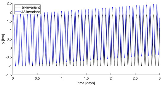
Figure 10. Mid-inclination eccentric LEO formation: time behavior of y component for $J_n$-invariant and $J_2$-invariant initial conditions.

4.3. Formation in Medium-Inclination Lunar Orbit

The effectiveness of the model is evaluated in the extremely perturbed lunar gravitational field [38], examining the stability of a formation designed for the purpose of lunar navigation [39,40], with parameters indicated in Table 10 and the $J_n$-invariant initial state reported in Table 11. The relative trajectory is shown in Figure 11 and it can be compared to the one obtained from a non-invariant initial state, shown in Figure 12. Table 12 collects the extreme values for the position coordinates during the first and the last orbit, corresponding to a negligible increase in the amplitude of both the in-plane and the out-of-plane oscillations of 0.48% and 0.16%. As highlighted by Figure 13, the use of $J_n$-invariant initial conditions ensures the stability of the boundedness condition, mitigating the drift, which is reduced to a negligible value.

Table 10. Lunar formation: orbit parameters of chief satellite.

semimajor axis	$\overline{a}$	6038 km
eccentricity	e	0
inclination	i	40${}^{\circ }$
RAAN	$\mathrm{\Omega }$	0
epoch (UTC)	-	24 January 2023 12:00:00

Table 11. Lunar formation: initial state of deputy satellite.

Hamiltonian Variables		Position/Velocity Components
$w_1$	0	x	8.5390 km
$w_2$	j ·${10}^{-3}$	y	−17.0780 km
$w_3$	(1 + j) ·${10}^{-4}$	z	0.8539 km
$z_1$	0	$v_x$	−1.2744 m/s
$z_2$	−1 ·${10}^{-3}$	$v_y$	−2.5523 m/s
$z_3$	(−1 − j) · ${10}^{-4}$	$v_z$	−0.1274 m/s

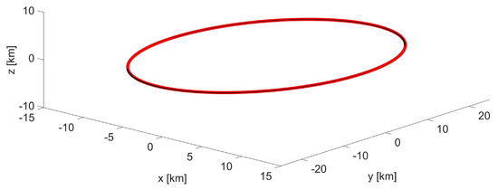
Figure 11. Lunar formation: $J_n$-invariant bounded trajectory (black) in ${\mathcal{F}}_r$; the first orbit is plotted in red.

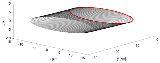
Figure 12. Lunar formation: trajectory (black) in ${\mathcal{F}}_r$ resulting from non-invariant initial conditions; the first orbit is plotted in red.

Table 12. Lunar formation: maximum and minimum value of the position coordinates for the first and the last orbit.

First Orbit		Last Orbit
$x^{max}$	12.0678 km	$x^{max}$	12.0679 km
$x^{min}$	−12.0669 km	$x^{min}$	−12.0673 km
$y^{max}$	24.0799 km	$y^{max}$	24.0799 km
$y^{min}$	−24.1878 km	$y^{min}$	−24.4185 km
$z^{max}$	1.2091 km	$z^{max}$	1.2103 km
$z^{min}$	−1.2043 km	$z^{min}$	−1.2055 km

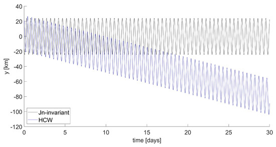
Figure 13. Lunar formation: time behavior of y component.

4.4. Injection into a Relative Bounded Trajectory

The guidance strategy proposed in Section 3.4 is implemented here to inject a reconnaissance satellite $S{C}_2$ into an invariant bounded trajectory about the target object $S{C}_1$, characterized by the orbit parameters reported in Table 13 and Table 14. Data in these tables allow determining the relative position and velocity of $S{C}_2$ in ${\mathcal{F}}_r$ at the initial epoch and, consequently, the corresponding state in Hamiltonian variables, collected in Table 15.

Table 13. Guidance strategy: orbit parameters of target object.

semimajor axis	$\overline{a}$	6828 km
eccentricity	e	0
inclination	i	62 deg
RAAN	$\mathrm{\Omega }$	0 deg
true anomaly	$\theta$	0 deg
epoch (UTC)	-	24 January 2023 12:00:00

Table 14. Guidance strategy: orbit parameters of reconnaissance satellite.

semimajor axis	$\overline{a}$	6835 km
eccentricity	e	0.033
inclination	i	62 deg
RAAN	$\mathrm{\Omega }$	$359.9$ deg
argument of perigee	$\omega$	$92.4$ deg
true anomaly	$\theta$	$267.5$ deg
epoch (UTC)	-	24 January 2023 12:00:00

Table 15. Guidance strategy: initial state of reconnaissance satellite.

Hamiltonian Variables		Position/Velocity Components
$w_1$	$-{10}^{-4}$	x	9.6562 km
$w_2$	(0.11 − 2.04j) · ${10}^{-2}$	y	−19.3123 km
$w_3$	(1 + j) · ${10}^{-3}$	z	9.6563 km
$z_1$	−3 · ${10}^{-4}$	$v_x$	−242.2476 m/s
$z_2$	(2.04 − 0.11j) · ${10}^{-2}$	$v_y$	−21.1209 m/s
$z_3$	(−1 − j) · ${10}^{-3}$	$v_z$	−1.2055 m/s

Developing the transformation ${\mathcal{T}}_7$, it can be verified that the coefficients of matrix ${\mathbf{T}}_N$ for the case examined here are $c_1=\frac{\sqrt{2}}{2}$, $c_2=-8.2241·{10}^{-4}$, and $c_3=607.9516$; then, applying Equation (37) with $w_1$ and $z_1$ in Table 15 provides $\delta v_x=231.442$ m/s and $\delta v_y=-0.542$ m/s. According to Equation (39), such a $\mathrm{\Delta }V$ provided at the initial time is the minimum one; the state resulting from the maneuver is reported in Table 16 and the complete trajectory is shown in Figure 14. It is worth emphasizing here that the transfer of a spacecraft into a bounded relative trajectory only requires an in-plane change in velocity. Figure 15 shows details of the injection point in which an arrow indicates the direction of the $\mathrm{\Delta }V$ provided, which lies on the $\left[\begin{array}{cc}\widehat{x}& \widehat{y}\end{array}\right]$ plane. As expected from the theory, a change in the in-plane velocity components does not affect the out-of-plane dynamics. In fact, the values of $w_3$ and $z_3$ in Table 15 are the same as in Table 16, and the amplitude of the z component does not vary after the maneuver, as shown in Figure 16.

Table 16. Lunar formation: state of reconnaissance satellite after the maneuver.

Hamiltonian Variables		Position/Velocity Components
$w_1$	0	x	9.6562 km
$w_2$	(1 + j) ·${10}^{-3}$	y	−19.3123 km
$w_3$	(1 + j) ·${10}^{-3}$	z	9.6563 km
$z_1$	0	$v_x$	−10.8052 m/s
$z_2$	(−1 − j) · ${10}^{-3}$	$v_y$	−21.6630 m/s
$z_3$	(−1 − j) · ${10}^{-3}$	$v_z$	−1.2060 m/s

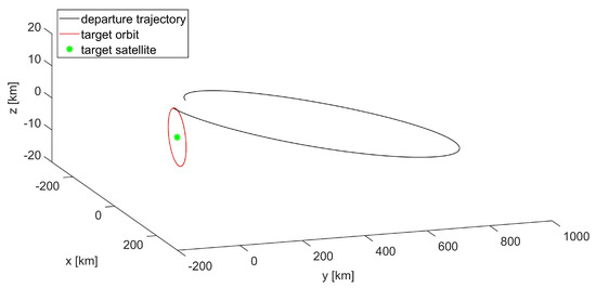
Figure 14. Guidance strategy: transfer of the reconnaissance satellite into a $J_n$-invariant bounded trajectory in ${\mathcal{F}}_r$ about the target object.

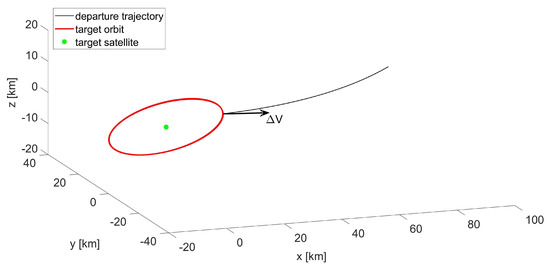
Figure 15. Guidance strategy: detail of the injection point between the departure trajectory and the target orbit in ${\mathcal{F}}_r$; the arrow indicates the direction of the $\mathrm{\Delta }V$ provided.

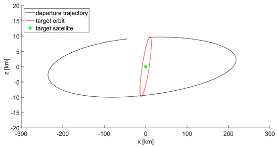
Figure 16. Guidance strategy: projection of the trajectory onto the $\left[\begin{array}{cc}\widehat{x}& \widehat{z}\end{array}\right]$ plane; the amplitude of the z component does not change after the maneuver.

5. Conclusions

This research introduces a novel model which provides a compact representation of relative trajectories invariant under the zonal harmonic perturbation. This solution is developed using the Hamiltonian formalism where canonical transformations allow reducing the dynamics of the perturbed problem to a form equivalent to that of the unperturbed one, without requiring any truncation of the zonal harmonic coefficients. In the transformed coordinates, formation configurations with the desired drift behavior and amplitude of the oscillations can be designed based only on four parameters that can be rapidly converted to the corresponding relative position and velocity coordinates; a few algebraic operations are enough to determine $J_n$-invariant relative trajectories, and the model does not require any further numerical refinement.

The accuracy of the solution is evaluated through numerical integration, using high-fidelity orbit propagators (JGM-2, LP-165, DE405) on initial states generated by the model for some scenarios of interest: Earth SSO, medium-inclination LEO, and a medium-inclination lunar orbit. The results of the analysis indicate that the parameters of the relative trajectory are stable, with the amplitude of the oscillations varying by less than 4% of their initial value over 30 days and the drift being negligible.

Based on the geometric properties of the transformed Hamiltonian system, a guidance strategy is developed to inject a spacecraft into a stable bounded relative trajectory about another orbiting object nearby. Furthermore, this strategy is verified numerically, proving its effectiveness in establishing the transfer between relative trajectories once provided the $\mathrm{\Delta }V$ indicated by the theoretical analysis.

Appendix A.1. Lagrangian for the Relative Motion under the Zonal Harmonic Perturbation

The reader shall recall from Section 2 that the relative coordinates of the deputy satellite with respect to the chief are expressed in the reference frame ${\mathcal{F}}_r$, using the symbol $\rho$ to indicate the relative position. ${\mathcal{F}}_r$ rotates with respect to an Earth-centered inertial (ECI) frame with an angular velocity $\omega$ depending on both the orbit angular speed n of the chief satellite and that of its orbit plane caused by the gravitational perturbations. The expression of ${\mathcal{L}}_r$ is here developed considering only the secular effect of $J_2$ on the rotation of the orbit plane, which causes the time drift in the RAAN and in the argument of latitude expressed below:

$$\dot{\mathrm{\Omega }}=-\frac{3}{2}n{J}_2{\left(\frac{R_E}{\overline{r}}\right)}^{2}cosi$$

(A1)

$$\dot{u}=n+\delta n$$

(A2)

with

$$n=\sqrt{\frac{\mu }{{\overline{a}}^3}}$$

(A3)

$$\delta n=\frac{3}{4}n{J}_2{\left(\frac{R_E}{\overline{r}}\right)}^2\left(3-\frac{7}{2}{sin}^{2}i\right)$$

(A4)

$$\overline{r}=\overline{a}+\frac{3}{4}{J}_2{\left(\frac{R_E}{\overline{a}}\right)}^2\left(3{sin}^{2}i-2\right)$$

(A5)

where $\overline{r}$ is the mean radius of the $J_2$-perturbed orbit, $\overline{a}$ is the semi-major axis, and i is the inclination of the orbital plane. Based on Equations (A1)–(A5), the expression of $\omega$ is given by

$$\omega =\left[\begin{array}{c}\dot{\mathrm{\Omega }}sinisinu\\ \dot{\mathrm{\Omega }}sinicosu\\ \dot{\mathrm{\Omega }}cosi+\dot{u}\end{array}\right]$$

(A6)

Equation (A6) is now used to derive the expression for the relative velocity in the inertial frame, reported below, and that of the relative kinetic energy $K_r$.

$$\mathbf{v}=\omega \times \overline{\mathbf{r}}+\frac{d\rho }{dt}+\omega \times \rho$$

(A7)

For the sake of compactness, it is worth isolating from Equation (A7) the terms ${\mathbf{v}}^{\left(1\right)}$, used in Equation (4), depending on the perturbation (i.e., on $J_2$).

$$\mathbf{v}={\mathbf{v}}^{\left(0\right)}+{\mathbf{v}}^{\left(1\right)}$$

(A8)

where

$$v^{\left(0\right)}=\left[\begin{array}{c}\dot{x}-ny\\ \dot{y}+nx+n\overline{r}\\ \dot{z}\end{array}\right]$$

(A9)

and

$$v^{\left(1\right)}=\left[\begin{array}{c}\dot{\mathrm{\Omega }}\left(zsinicosu-ycosi\right)-y\delta n\\ \left(\dot{\mathrm{\Omega }}cosi+\delta n\right)\left(x+\overline{r}\right)-z\dot{\mathrm{\Omega }}sinisinu\\ \dot{\mathrm{\Omega }}sini\left(ysinu-(x+\overline{r})cosu\right)\end{array}\right]$$

(A10)

Finally, the relative kinetic energy can be expressed in compact form based on Equations (A8)–(A10):

$$K_r=\frac{1}{2}|v^{\left(0\right)}{|}^2+v^{{\left(0\right)}^T}{v}^{\left(1\right)}+\frac{1}{2}{\left|v^{\left(1\right)}\right|}^2$$

(A11)

Once the expression of $K_r$ is derived, an equivalent representation of the relative potential $V_r$ is necessary to obtain the Lagrangian. As suggested by Kolemen et al. [17], the expression of $V_r$, including the zonal harmonic coefficient, can be obtained after expressing Equation (2) for $S{C}_2$ and $S{C}_1$ in ${\mathcal{F}}_r$ and then subtracting the two, resulting in the following form:

$$V_r=-\frac{\mu }{\overline{r}+\rho }\left[1-\sum _{n=2}^{\infty }{J}_n{\left(\frac{R_E}{\overline{r}+\rho }\right)}^n{P}_n(cos\varphi )\right]$$

(A12)

The geocentric co-latitude $\varphi$ can be obtained from the projection of $\mathbf{r}=\overline{r}{\widehat{r}}_1+\rho$ along the ${\widehat{c}}_3$ axis of the ECI frame, expressed through the 3-1-3 rotation ${\mathcal{R}}_{ri}={\mathcal{R}}_3^T\left(\mathrm{\Omega }\right){\mathcal{R}}_1^T\left(i\right){\mathcal{R}}_3^T\left(u\right)$:

$$cos\varphi =\frac{(\overline{\mathbf{r}}+\rho ){\mathcal{R}}_{ri}^T{\widehat{c}}_3}{\overline{r}+\rho }=\left[\begin{array}{ccc}sinisinu& sinicosu& cosi\end{array}\right]\frac{\overline{\mathbf{r}}+\mathbf{\rho }}{\overline{r}+\rho }$$

(A13)

We can then introduce Equation (A13) into Equation (A12) and set

$$\frac{1}{\overline{r}+\rho }=\frac{1}{\overline{r}\sqrt{1-2\frac{\rho }{\overline{r}}cos\beta +{\left(\frac{\rho }{\overline{r}}\right)}^2}}$$

(A14)

where

$$cos\beta =-\frac{{\mathbf{\rho }}^T\overline{\mathbf{r}}}{\rho \overline{r}}=-\frac{x}{\rho }$$

(A15)

The expression of $V_r$ can be approximated using the Legendre polynomials

$$\frac{1}{\overline{r}+\rho }=\sum _{k=0}^{\infty }\left[\frac{1}{2^{k}K!}\frac{d^k{({cos}^2\beta -1)}^k}{d{(cos\beta )}^k}{\left(\frac{\rho }{\overline{r}}\right)}^k\right]$$

(A16)

As detailed in Appendix A.2, because $\rho <<\overline{r}$, Equation (A16) can be truncated to the second order in $\frac{\rho }{\overline{r}}$, obtaining

$$\frac{1}{\overline{r}+\rho }=-\frac{1}{\overline{r}}\left[1+\frac{\rho }{\overline{r}}cos\beta +{\left(\frac{\rho }{\overline{r}}\right)}^2\left(\frac{3}{2}{cos}^2\beta -\frac{1}{2}\right)\right]$$

(A17)

and

$$cos\varphi =\frac{1}{\overline{r}}\left[1+\frac{\rho }{\overline{r}}cos\beta +{\left(\frac{\rho }{\overline{r}}\right)}^2\left(\frac{3}{2}{cos}^2\beta -\frac{1}{2}\right)\right]\left[\left(x+\overline{r}\right)sinisinu+ysinicosu+zcosi\right]$$

(A18)

Finally, introducing Equations (A17)–(A18) into Equation (A12) and subtracting $V_r$ to $K_r$ results in the following expression for the Lagrangian of the problem:

$${\mathcal{L}}_r={\mathcal{L}}_r^{\left(0\right)}+{\mathcal{L}}_r^{\left(k\right)}$$

(A19)

with

$${\mathcal{L}}_r^{\left(0\right)}=\frac{{\left(\dot{x}-ny\right)}^2}{2}+\frac{{\left(\dot{y}+\overline{r}n+nx\right)}^2}{2}+\frac{{\dot{z}}^2}{2}+\left(n^2{\overline{r}}^2\right)\left(1-\frac{x}{\overline{r}}+\frac{3}{2}\frac{x^2}{{\overline{r}}^2}-\frac{1}{2}\frac{\left(x^2+y^2+z^2\right)}{{\overline{r}}^2}\right)$$

(A20)

$${\mathcal{L}}_r^{\left(k\right)}={\dot{x}}^{\left(1\right)}\left(\dot{x}-ny\right)-{\dot{y}}^{\left(1\right)}\left(\dot{y}+\overline{r}n+nx\right)+{\dot{z}}^{\left(1\right)}\dot{z}+{\left({\dot{x}}^{\left(1\right)}\right)}^2+{\left({\dot{y}}^{\left(1\right)}\right)}^2+{\left({\dot{z}}^{\left(1\right)}\right)}^2+f\left(J_n^k,\frac{\rho }{\overline{r}},\frac{{\rho }^2}{{\overline{r}}^2}\right)$$

(A21)

where ${\mathbf{v}}^{\left(1\right)}={\left[\begin{array}{ccc}{\dot{x}}^{\left(1\right)}& {\dot{y}}^{\left(1\right)}& {\dot{z}}^{\left(1\right)}\end{array}\right]}^T$ and $f\left(J_n^k,\frac{\rho }{\overline{r}},\frac{{\rho }^2}{{\overline{r}}^2}\right)$ collects the terms depending on the $J_n$ coefficients, which shall be selected as detailed in the following section. The term ${\mathcal{L}}^{\left(0\right)}$ of the Lagrangian corresponds to the one for the unperturbed problem and the HCW equations can be derived applying the Euler–Lagrange equation $\frac{d}{dt}\left(\frac{\partial {\mathcal{L}}_r^{\left(0\right)}}{\partial \dot{\rho }}\right)-\frac{\partial {\mathcal{L}}_r^{\left(0\right)}}{\partial \rho }=0$.

Appendix A.2. Scale Analysis

The expression of ${\mathcal{L}}_r$ derived in the previous section includes the Legendre polynomials up to order $k=2$, based on the hypothesis that $\frac{\rho }{\overline{r}}<<1$. In fact, when examining the problem under the zonal harmonic perturbation, values of interest for $\overline{r}$ are those corresponding to LEO altitudes $h\in \left[400,700\right]$ km, while values of the relative distances are typically in the range $\rho \in \left[1,1000\right]$ km. Consequently, for $k=2$ the truncation error is always lower than $2.2·{10}^{-2}$, an acceptable value which substantiates the approximation. Equivalent results can be obtained considering low lunar orbits.

A similar analysis is extended to the zonal harmonic coefficients to identify the ones to include in the model for providing adequately accurate results. It shall be observed that ${\left(\frac{\rho }{\overline{r}}\right)}^2\in \left[2.0·{10}^{-8},2.2·{10}^{-2}\right]$; thus, all the combinations of zonal harmonic coefficients in this range shall be taken into account in the analysis. According to the JGM-2 Earth gravity model [35], the following coefficients were considered for the analysis in Section 4.1, Section 4.2, and Section 4.4: $J_2–J_{14}$ and $J_{23}$.

Similarly for the Moon, ${\left(\frac{\rho }{\overline{r}}\right)}^2\in \left[3.3·{10}^{-7},3.3·{10}^{-1}\right]$, so all the combinations of zonal harmonic coefficients in this range shall be considered and, according to the LP-165 Moon gravity model [36], the following coefficients were included in the analysis in Section 4.3: $J_2$–$J_4$, $J_6$–$J_{12}$, $J_{14}$, $J_{16}$–$J_{18}$, $J_{20}$, $J_{27}$–$J_{29}$, $J_{31}$–$J_{32}$.

Appendix A.3. Hamiltonian Formalism

The Hamiltonian formalism allows representing the relative dynamics of satellites in close proximity in terms of the Hamiltonian variables $\mathbf{q}=\mathbf{\rho }$ and $\mathbf{p}=\frac{\partial {\mathcal{L}}_r}{\partial {\mathbf{v}}^T}$, explained by Equations (4). The Hamiltonian function is obtained by applying the Legendre transformation to the Lagrangian

$$H={\dot{\mathbf{\rho }}}^T\mathbf{p}-{\mathcal{L}}_r$$

(A22)

leading to

$$H=H^{\left(0\right)}\left(\mathbf{q},\mathbf{p}\right)+H^{\left(k\right)}\left(\mathbf{q},\mathbf{p},J_n^k\right)$$

(A23)

where

$$H^{\left(0\right)}=\frac{1}{2}{\left(p_x+ny\right)}^2+\frac{1}{2}{\left(p_y-\overline{a}n-nx\right)}^2+\frac{p_z^2}{2}-\frac{3}{2}{n}^2{x}^2+n^2\frac{z^2}{2}$$

(A24)

$$H^{\left(k\right)}=-{\mathbf{v}}^{\left(1\right)}·\mathbf{q}+f\left(\mathbf{q},J_n^k\right)$$

(A25)

where, as for Equation (A21), the terms depending on the zonal harmonic coefficients are collected in $f\left(\mathbf{q},J_n^k\right)$.

To improve the numerical processing, Equations (A23)–(A25) are converted to a dimensionless form

$$\left\{\begin{array}{c}\widehat{\mathbf{q}}=\frac{\mathbf{q}}{DU}\hfill \\ \widehat{\mathbf{p}}=\mathbf{p}\frac{TU}{DU}\hfill \end{array}\right.$$

(A26)

where $DU=\overline{a}$ and $TU=1/n$ are the units of distance and time.

$$H^{\left(0\right)}=\frac{1}{2}{\left({\widehat{p}}_x+\widehat{y}\right)}^2+\frac{1}{2}{\left({\widehat{p}}_y-1-\widehat{x}\right)}^2+\frac{{\widehat{p}}_z^2}{2}-\frac{3}{2}{\widehat{x}}^2+\frac{{\widehat{z}}^2}{2}$$

(A27)

$$H^{\left(k\right)}=-{\widehat{\mathbf{v}}}^{\left(1\right)}·\widehat{\mathbf{q}}+\widehat{f}\left(\widehat{\mathbf{q}},J_n^k\right)$$

(A28)

Finally, considering the results of the scale analysis in Appendix A.2, the expression of $H^{\left(k\right)}$ can be rearranged as the sum of two terms, $H^{\left(1\right)}$ and $H^{\left(2\right)}$, collecting, respectively, the zonal coefficients $J_n$ and $J_n^2$. The complete expression of H in dimensionless form is given by Equations (5)–(8), where the hat sign was discarded to ease the notation.

References

- Bandyopadhyay, S.; Subramanian, G.P.; Foust, R.; Morgan, D.; Chung, S.J.; Hadaegh, F.Y. A Review of Impending Small Satellite Formation Flying Missions. In Proceedings of the 53rd AIAA Aerospace Sciences Meeting, Kissimmee, FL, USA, 5–9 January 2015; Volume 53, pp. 567–578. [Google Scholar] [CrossRef]
- Chung, S.J.; Bandyopadhyay, S.; Foust, R.; Subramanian, G.P. Review of Formation Flying and Constellation Missions Using Nanosatellites. J. Spacecr. Rocket. 2016, 53, 567–578. [Google Scholar] [CrossRef]
- ESA Space Debris Office. ESA’S Annual Space Environment Report; ESA Space Debris Office: Darmstadt, Germany, 2022. [Google Scholar]
- Vinti, J.P. Zonal Harmonic Perturbations of an Accurate Reference Orbit of an Artificial Satellite. J. Res. Natl. Bur. Stand. Math. Math. Phys. 1963, 67B, 191–222. [Google Scholar] [CrossRef]
- Wnuk, E. Second order perturbations due to the gravity potential of a planet. In From Newton to Chaos; Roy, A.E., Stevens, B.A., Eds.; Plenum Press: New York, NY, USA, 1995; pp. 259–260. [Google Scholar]
- Djojodihardjo, H. Influence of the Earth’s Dominant Oblateness Parameter on the Low Formation Orbits of Micro-Satellites. Int. J. Automot. Mech. Eng. 2014, 9, 1802–1819. [Google Scholar] [CrossRef]
- Wu, B.; Wang, D.; Poh, E.K. Dynamic Models of Satellite Relative Motion Around an Oblate Earth. In Satellite Formation Flying. Intelligent Systems, Control and Automation: Science and Engineering; Springer: Singapore, 2016; Volume 87, pp. 9–41. [Google Scholar] [CrossRef]
- Prussing, J.A.; Conway, B.A. Orbital Mechanics; Oxford University Press: New York, NY, USA, 1993; pp. 139–152. [Google Scholar]
- Burnett, E.R.; Schaub, H. Study of highly perturbed spacecraft formation dynamics via approximation. Adv. Space Res. 2021, 67, 3381–3395. [Google Scholar] [CrossRef]
- Izzo, D.; Sabatini, M.; Palmerini, G. Minimum control for spacecraft formations in a J2 perturbed environment. Celest. Mech. Dyn. Astron. 2009, 105, 141–157. [Google Scholar] [CrossRef]
- Bando, M.; Ichikawa, A. In-Plane Motion Control of Hill–Clohessy–Wiltshire Equations by Single Input. J. Guid. Control. Dyn. 2013, 36, 1512–1521. [Google Scholar] [CrossRef]
- Agarwal, S.; Sinha, A. Formation Control of Spacecraft under orbital perturbation. IFAC—PapersOnLine 2016, 49, 130–135. [Google Scholar] [CrossRef]
- Armellin, R. Collision avoidance maneuver optimization with a multiple-impulse convex formulation. Acta Astronaut. 2021, 186, 347–362. [Google Scholar] [CrossRef]
- Andrievsky, B.; Popov, A.M.; Kostin, I.; Fadeeva, J. Modeling and Control of Satellite Formations: A Survey. Automation 2022, 3, 511–544. [Google Scholar] [CrossRef]
- Schaub, H.; Alfriend, K. J2 Invariant Relative Orbits for Spacecraft Formations. Celest. Mech. Dyn. Astron. 2001, 79, 77–95. [Google Scholar] [CrossRef]
- Schweighart, S.A.; Sedwick, R.J. High-Fidelity Linearized J2 Model for Satellite Formation Flight. J. Guid. Control. Dyn. 2002, 25, 1073–1091. [Google Scholar] [CrossRef]
- Kolemen, E.; Kasdin, N.J.; Gurfil, P. Hamilton-Jacobi modelling of relative motion for formation flying. Ann. N. Y. Acad. Sci. 2005, 1065, 93–111. [Google Scholar] [CrossRef] [PubMed]
- Sabatini, M.; Izzo, D.; Bevilacqua, R. Special Inclinations Allowing Minimal Drift Orbits for Formation Flying Satellites. J. Guid. Control. Dyn. 2008, 31, 94–100. [Google Scholar] [CrossRef]
- He, Y.; Armellin, R.; Xu, M. Bounded Relative Orbits in the Zonal Problem via High-Order Poincaré Maps. J. Guid. Control. Dyn. 2018, 42, 91–109. [Google Scholar] [CrossRef]
- Ma, Y.; He, Y.; Xu, M.; Zhou, Q.; Chen, X. Invariant relative orbits for spacecraft formation flying in high-order gravitational field. Acta Astronaut. 2021, 189, 398–428. [Google Scholar] [CrossRef]
- Deprit, A.; Henrard, J. Canonical transformations depending on a small parameter. Celest. Mech. 1969, 1, 12–30. [Google Scholar] [CrossRef]
- Carletta, S.; Pontani, M.; Teofilatto, P. Design of low-energy capture trajectories in the elliptic restricted four-body problem. In Proceedings of the 70th International Astronautical Congress, Washington DC, USA, 21–25 October 2019. [Google Scholar]
- del Portillo, I.; Cameron, B.; Crawley, E. A technical comparison of three low earth orbit satellite constellation systems to provide global broadband. Acta Astronaut. 2019, 159, 123–135. [Google Scholar] [CrossRef]
- Schilling, K. Mission Analyses for Low-Earth-Observation Missions with Spacecraft Formations. RTO Educ. Notes Pap. 2011, 231. [Google Scholar]
- Knobelspiesse, K.; Nag, S. Remote sensing of aerosols with small satellites in formation flight. Atmos. Meas. Tech. 2018, 11, 3935–3954. [Google Scholar] [CrossRef]
- Martorella, M.; Giusti, E.; Gelli, S.; Tomei, S.; Atle-Onar, K.; Palmerini, G.; Teofilatto, P.; Nascetti, A.; Pisa, S.; Eriksen, T.; et al. Spaceborne SAR Cluster. In Proceedings of the AVT-336 Research Specialists’ Meeting on Enabling Platform Technologies for Resilient Small Satellite Constellation for NATO Missions, Virtual, Online, 11–14 October 2021. [Google Scholar]
- Ely, T.; Lieb, E. Constellations of Elliptical Inclined Lunar Orbits Providing Polar and Global Coverage. In Proceedings of the AAS/AIAA Astrodynamics Specialists Conference, Lake Tahoe, CA, USA, 7–11 August 2005. [Google Scholar]
- Leonardi, M. Geometrical comparison of different localization methods for lunar navigation exploiting ELFO and Halo orbits. In Proceedings of the 73rd International Astronautical Congress, Paris, France, 18–22 September 2022. [Google Scholar]
- Sirbu, G.; Leonardi, M.; Carosi, M.; Di Lauro, C.; Stallo, C. Performance evaluation of a lunar navigation system exploiting four satellites in ELFO orbits. In Proceedings of the 2022 IEEE 9th International Workshop on Metrology for AeroSpace, Pisa, Italy, 27–29 June 2022. [Google Scholar]
- Kozai, Y. Tesseral harmonics of the gravitational potential of the earth as derived from satellite motions. Astron. J. 1961, 66, 355–358. [Google Scholar] [CrossRef]
- Carletta, S.; Pontani, M.; Teofilatto, P. Characterization of Low-Energy Quasiperiodic Orbits in the Elliptic Restricted 4-Body Problem with Orbital Resonance. Aerospace 2022, 9, 175. [Google Scholar] [CrossRef]
- Siegel, C.; Moser, J. Lectures on Celestial Mechanics; Reprint of the 1971 Edition; Springer: Berlin, Germany, 1995. [Google Scholar] [CrossRef]
- Carletta, S.; Pontani, M.; Teofilatto, P. Station-keeping about Sun-Mars three-dimensional quasi-periodic Collinear Libration Point Trajectories. Adv. Astronaut. Sci. 2020, 173, 299–311. [Google Scholar]
- Standish, E.; Newhall, X.; Williams, J.; Folkner, W. JPL Planetary and Lunar Ephemerides; Willmann-Bell, Inc.: Richmond, VA, USA, 1997. [Google Scholar]
- Nerem, R.S.; Lerch, F.J.; Marshall, J.A.; Pavlis, E.C.; Putney, B.H.; Tapley, B.D.; Eanes, R.J.; Ries, J.C.; Schutz, B.E.; Shum, C.K.; et al. Gravity model development for TOPEX/POSEIDON: Joint Gravity Models 1 and 2. J. Geophys. Res. 1994, 99, 421–447. [Google Scholar] [CrossRef]
- Konopliv, A.; Asmar, S.; Carranza, E.; Sjogren, W.; Yuan, D. Recent Gravity Models as a Result of the Lunar Prospector Mission. Icarus 2001, 150, 1–18. [Google Scholar] [CrossRef]
- Kulik, J. An in-plane J2-invariance condition and control algorithm for highly elliptical satellite formations. Celest. Mech. Dyn. Astron. 2021, 133, 4. [Google Scholar] [CrossRef]
- Graziani, F.; Sparvieri, N.; Carletta, S. A low-cost earth-moon-mars mission using a microsatellite platform. In Proceedings of the 71st International Astronautical Congress, Virtual, Online, 12–14 October 2020. [Google Scholar]
- Thompson, J.; Hunter, G.; Keziram, M. Design and Analysis of Lunar Communication and Navigation Satellite Constellation Architectures. In Proceedings of the AIAA SPACE 2010 Cyberspace & Exposition, Anaheim, CA, USA, 30 August–2 September 2010; pp. 190–200. [Google Scholar] [CrossRef]
- Carletta, S. Design of fuel-saving lunar captures using finite thrust and gravity-braking. Acta Astronaut. 2021, 181, 190–200. [Google Scholar] [CrossRef]
Disclaimer/Publisher’s Note: The statements, opinions and data contained in all publications are solely those of the individual author(s) and contributor(s) and not of MDPI and/or the editor(s). MDPI and/or the editor(s) disclaim responsibility for any injury to people or property resulting from any ideas, methods, instructions or products referred to in the content. |
© 2023 by the author. Licensee MDPI, Basel, Switzerland. This article is an open access article distributed under the terms and conditions of the Creative Commons Attribution (CC BY) license (https://creativecommons.org/licenses/by/4.0/).