Implicit Bias of Deep Learning in the Large Learning Rate Phase: A Data Separability Perspective

Abstract

Previous literature on deep learning theory has focused on implicit bias with small learning rates. In this work, we explore the impact of data separability on the implicit bias of deep learning algorithms under the large learning rate. Using deep linear networks for binary classification with the logistic loss under the large learning rate regime, we characterize the implicit bias effect with data separability on training dynamics. From a data analytics perspective, we claim that depending on the separation conditions of data, the gradient descent iterates will converge to a flatter minimum in the large learning rate phase, which results in improved generalization. Our theory is rigorously proven under the assumption of degenerate data by overcoming the difficulty of the non-constant Hessian of logistic loss and confirmed by experiments on both experimental and non-degenerated datasets. Our results highlight the importance of data separability in training dynamics and the benefits of learning rate annealing schemes using an initial large learning rate.

1. Introduction

Deep neural networks have proven to be highly effective in both supervised and unsupervised learning tasks. Theoretical understanding of the mechanisms underlying deep learning’s power is continuously evolving and expanding. Recent progress in deep learning theory has shown that over-parameterized networks can achieve very low or zero training error through gradient descent-based optimization [1,2,3,4,5,6]. Surprisingly, these over-parameterized networks can also generalize well to the test set, a phenomenon known as double descent [7]. One promising explanation for this phenomenon is implicit bias [8] or implicit regularization [9], which is characterized by maximum margin. A large family of works has studied exponential tailed losses, such as logistic and exponential loss, and reported implicit regularization of maximum margin [8,10,11,12,13].

However, the current theoretical understanding of the optimization and generalization properties of deep learning models is limited due to the assumption of small learning rates in existing theoretical results on implicit bias. In practice, using a large initial learning rate in a learning rate annealing scheme has been shown to result in improved performance. The relationship between data separability and implicit bias during the large learning rate phase remains unclear [14,15]. To address this gap, we examine the effect of the large learning rate on deep linear networks with logistic and exponential loss.

Ref. [16] shed light on the large learning rate phase by observing a distinct phenomenon that the local curvature of the loss landscape drops significantly in the large learning rate phase and thus typically can obtain the best performance. By following [16], we characterize the gradient descent training in terms of three learning rate regimes or phases. (i) Lazy phase $\eta <{\eta }_0$, when the learning rate is small, the dynamics of a neural network under a linearized dynamics regime, where a model converges to a nearby point in parameter space called lazy training and characterized by the neural tangent kernel [1,2,3,17,18,19]. (ii) Catapult phase ${\eta }_0<\eta <{\eta }_1$, the loss grows at the beginning and then drops until it converges to the solution with a flatter minimum. (iii) Divergent phase $\eta >{\eta }_1$, the loss diverges and the model does not train. The importance of the catapult phase increases because the lazy phase is generally detrimental to generalization and does not explain the practically observed power of deep learning [20,21].

While the phenomenon of the three learning rate phases is reported in a regression setting with mean-squared-error (MSE) loss, it remains unclear whether this can be extended to cross-entropy (logistic) loss along with the data separability. To fill this gap, we examine the effect of a large learning rate on deep linear networks with logistic and exponential loss. Contrary to MSE loss, the characterization of gradient descent with logistic loss concerning learning rate is associated with separation conditions of the data. In addition, the major difficulty is that a non-constant Hessian makes it difficult to draw the boundaries of the catapult phase in the classification settings. Meanwhile, the changes in dynamics have become more complicated, making it difficult to analyse. Our results are different from [16] in many aspects. First, a non-constant Hessian brings more technical challenges. Second, the appearance the catapult phase under logistic loss depends on the separability of the dataset, while squared loss has no such condition. Third, we observed oscillations in the dynamics of training loss in Figure 1, which is not observed in MSE loss. Finally, we summarize our contribution as follows:

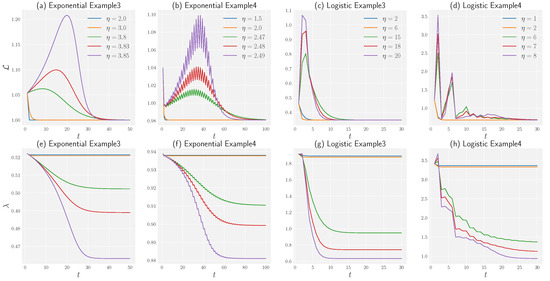
Figure 1. Dependence of dynamics of training loss and maximum eigenvalue of the NTK on the learning rate for a one-hidden-layer linear network, with (a,b,e,f) exponential loss and (c,d,g,h) logistic loss in Examples 3 and 4. (a–d) In a large learning rate regime (the catapult phase), the loss increases at the beginning and converges to a global minimum. (e–h) The maximum eigenvalue of the NTK decreases rapidly to a fixed value which is lower than its initial position in the large learning regime (the catapult phase).

• According to the separation conditions of the data, we characterize the dynamics of gradient descent with logistic and exponential loss corresponding to the learning rate. We find that the gradient descent iterates converge to a flatter minimum in the catapult phase when the data is non-separable. The above three learning rate phases do not apply to the linearly separable data since the optimum is towards infinity.
• Our theoretical analysis ranges from a linear predictor to a one-hidden-layer network. By comparing the convex optimization characterized by Theorem 1 and non-convex optimization characterized by Theorem A2 in terms of the learning rate, we show that the catapult phase is a unique phenomenon for non-convex optimizations.
• We find that in practical classification tasks, the best generalization results tend to occur in the catapult phase. Given the fact that the infinite-width analysis (lazy training) does not fully explain the empirical power of deep learning, our results can be used to partially fill this gap.
• Our theoretical findings were supported by extensive experimentation on the MNIST [22], CIFAR-10 [23] and CIFAR-100 datasets [24] with label noise, and the WebVision dataset [25].

2. Related Work

2.1. Implicit Bias of Gradient Methods

Since the seminal work from [8], implicit bias has led to a fruitful line of research. Works along this line have treated linear predictors [10,11,26,27]; deep linear networks with a single output [28,29,30] and multiple outputs [31,32]; homogeneous networks (including ReLU, max pooling activation) [12,13,33]; ultra wide networks [34,35,36]; and matrix factorization [31]. Notably, these studies adopt gradient flow (infinitesimal learning rate) or a sufficiently small learning rate.

2.2. Data Separability

In a recent review of data complexity measures, ref. [37] listed various measures for classification difficulty, including those based on the geometrical complexity of class boundaries. In a later survey by [38], most complexity measures were categorized into six groups: feature-based, linearity, neighbourhood, network, dimensionality, and class imbalance measures. Ref. [39] introduced the distance-based Ssparability index (DSI) to independently evaluate the data separability of the classifier model. The DSI indicates the degree to which data from different classes have similar distributions, which can make separation particularly challenging for classifiers. There has been limited attention given to combining data separability and the theory of implicit bias in deep learning. The noisy features can also impact data separability. The feature selection process is a type of dimensionality reduction that seeks to identify the most important features while discarding irrelevant or noisy features. Ref. [40] summarized how swarm intelligence-based feature selection methods are applied in different applications. Ref. [41] proposed the AGNMF-AN method seeking to improve upon existing methods for community detection by incorporating attribute information and using an adaptive affinity matrix.

2.3. Neural Tangent Kernel

Recently, we have witnessed exciting theoretical developments in understanding the optimization of ultra-wide networks, known as the neural tangent kernel (NTK) [1,2,3,5,17,18,19,42]. It is shown that in the infinite-width limit, NTK converges to an explicit limiting kernel, and it stays constant during training. Further, ref. [43] show that gradient descent dynamics of the original neural network fall into its linearized dynamics regime in the NTK regime. In addition, the NTK theory has been extended to various architectures such as orthogonal initialization [44], convolutions [17,45], graph neural networks [46,47], attention [48], PAC-Bayesian learning [6] and batch normalization [49] (see [50] for a summary). The constant property of NTK during training can be regarded as a special case of implicit bias, and importantly, it is only valid in the small learning rate regime.

2.4. Large Learning Rate and Logistic Loss

A large learning rate with SGD training is often set initially to achieve good performance in deep learning empirically [14,15,51]. The existing theoretical explanation of the benefit of the large learning rate contributes to two classes. One is that a large learning rate with SGD leads to flat minima [16,52,53], and the other is that the large learning rate acts as a regularizer [54]. Especially, [16] find a large learning rate phase can result in flatter minima without the help of SGD for mean squared loss. In this work, we ask whether the large learning rate still has this advantage with logistic loss. We expect a different outcome because the logistic loss is sensitive to the separation conditions of the data, and the loss surface is different from that of MSE loss [55].

3. Background

3.1. Setup

Consider a dataset ${\{x_i,y_i\}}_{i=1}^n$, with inputs $x_i\in {\mathbb{R}}^d$ and binary labels $y_i\in \{-1,1\}$. The empirical risk of the classification task follows the form,

$$\mathcal{L}=\frac{1}{n}\sum _{i=1}^n\ell \left(f\left(x_i\right)y_i\right),$$

(1)

where $f\left(x_i\right)$ is the output of the model corresponding to the input $x_i$, $\ell (·)$ is the loss function, and $\mathcal{L}$ is the empirical loss. Refer to Table 1 for the symbol description. In this work, we study two exponential tail losses which are exponential loss ${\ell }_{exp}\left(u\right)=exp(-u)$ and logistic loss ${\ell }_{log}\left(u\right)=log(1+exp(-u))$. The reason we look at these two losses together is that they are jointly considered in the realm of implicit bias by default [8]. We adopt gradient descent (GD) updates with learning rate $\eta$ to minimize empirical risk,

$$w_{t+1}=w_t-\eta \nabla \mathcal{L}\left(w_t\right)=w_t-\eta \sum _{i=1}^n{\ell }^{\prime }\left(f\left(x_i\right)y_i\right),$$

(2)

where $w_t$ is the parameter of the model at time step t.

Table 1. Key symbols and their definition.

Symbol	Definition
x	Input
y	Label
$\eta$	Learning rate
$\ell (·)$	Loss function
$\mathcal{L}$	Empirical loss
$w_t$	Parameters of the model at time step t
$\beta$	$\beta$-smooth convexity
$\alpha$	$\alpha$-strongly convexity
${\Theta }_{\alpha \beta }$	Neural Tangent Kernel

3.2. Separation Conditions of Dataset

It is known that landscapes of cross-entropy loss on linearly separable and non-separable data are different. Thus, the separation condition plays a crucial role in understanding the dynamics of gradient descent in terms of the learning rate. To build towards this, we define the two classes of separation conditions and review existing results for loss landscapes of a linear predictor in terms of separability.

Assumption 1.

The dataset is linearly separable, i.e., there exists a separator $w_{*}$ such that $\forall i:w_{*}^T{x}_i{y}_i>0$.

Assumption 2.

The dataset is non-separable, i.e., there is no separator $w_{*}$ such that $\forall i:w_{*}^T{x}_i{y}_i>0$.

Linearly separable. Consider the data under Assumption 1, one can examine that the loss of a linear predictor, i.e., $f\left(x\right)=w^{T}x$, is $\beta$-smooth convex with respect to w, and the global minimum is at infinity. The implicit bias of gradient descent with a sufficient small learning rate ($\eta <\frac{2}{\beta }$) in this phase was studied by [8]. They showed that the predictor converges to the direction of the maximum margin (hard margin SVM) solution, which implies the gradient descent method itself will find a proper solution with an implicit regularization instead of picking up a random solver. If one increases the learning rate until it exceeds $\eta <\frac{2}{\beta }$, then the result of converging to the maximum margin is not guaranteed, though loss can still converge to a global minimum.

Non-separable. Suppose we consider the data under Assumption 2, which is not linearly separable. The empirical risk of a linear predictor on these data are $\alpha$-strongly convex, and the global minimum is finite. In this case, given an appropriate small learning rate ($\eta <\frac{2}{\beta }$), the gradient descent converges towards the unique finite solution. When the learning rate is large enough, i.e., $\eta >\frac{2}{\alpha }$, we can rigorously show that gradient descent updates with this large learning rate leading to risk exploding or saturating.

We formally construct the relationship between loss surfaces and learning dynamics of gradient descent with respect to different learning rates on the two classes of data through the following proposition,

Proposition 1.

For a linear predictor $f=w^{T}x$, along with a loss $\ell \in \{{\ell }_{exp},{\ell }_{log}\}$.

1 

Under Assumption 1, the empirical loss is β-smooth. Then the gradient descent with constant learning rate $\eta <\frac{2}{\beta }$ never increases the risk, and empirical loss will converge to zero:

$$\mathcal{L}\left(w_{t+1}\right)-\mathcal{L}\left(w_t\right)\le 0,\underset{t\to \infty }{lim}\mathcal{L}\left(w_t\right)=0,with\eta <\frac{2}{\beta }.$$

2 

Under Assumption 2, the empirical loss is β-smooth and α-strongly convex, where $\alpha \le \beta$. Then the gradient descent with a constant learning rate $\eta <\frac{2}{\beta }$ never increases the risk, and empirical loss will converge to a global minimum. On the other hand, the gradient descent with a constant learning rate $\eta >\frac{2}{\alpha }$ never decreases the risk, and empirical loss will explode or saturate:

$$\begin{array}{cc}& \mathcal{L}\left(w_{t+1}\right)-\mathcal{L}\left(w_t\right)\le 0,\begin{array}{ccc}\hfill & \underset{t\to \infty }{lim}\mathcal{L}\left(w_t\right)=G_0,\hfill & \hfill with\eta <\frac{2}{\beta },\end{array}\hfill \\ & \mathcal{L}\left(w_{t+1}\right)-\mathcal{L}\left(w_t\right)\ge 0,\begin{array}{ccc}\hfill & \underset{t\to \infty }{lim}\mathcal{L}\left(w_t\right)=G_1,\hfill & \hfill with\eta >\frac{2}{\alpha },\end{array}\hfill \end{array}$$

where $G_0$ is the value of a global minimum while $G_1=\infty$ for exploding situation or $G_0<G_1<\infty$ when saturating.

4. Theoretical Results

4.1. Convex Optimization

It is known that the Hessian of the logistic and exponential loss with respect to the linear predictor is non-constant. Moreover, the estimated $\beta$-smooth convexity and $\alpha$-strongly convexity vary across different finite-bounded subspaces. As a result, the learning rate threshold in Proposition A1 is not detailed in terms of optimization trajectory. However, we can obtain more elaborate thresholds of the learning rate for a linear predictor by considering the degeneracy assumption:

Assumption 3.

The dataset contains two data points that have the same feature and opposite label, that is

$$(x_1=1,y_1=1)\mathrm{and}(x_2=1,y_2=-1).$$

We call this assumption the degeneracy assumption since the features from opposite label degenerate. Without loss of generality, we simplify the dimension of data and fix the position of the feature. Note that this assumption can be seen as a special case of non-separable data. Theoretical work has characterized general non-separable data [11], and we leave the analysis of this setting for the large learning rate to future work. Thanks to the symmetry of the risk function in space at the basis of degeneracy assumption, we can construct the exact dynamics of empirical risk with respect to the whole learning rate space.

Theorem 1.

For a linear predictor $f=w^{T}x$ equipped with an exponential (logistic) loss under Assumption 3, there is a critical learning rate that separates the whole learning rate space into two (three) regions. The critical learning rate satisfies

$${\mathcal{L}}^{\prime }\left(w_0\right)=-{\mathcal{L}}^{\prime }(w_0-{\eta }_{\mathrm{critical}}{\mathcal{L}}^{\prime }\left(w_0\right)),$$

where $w_0$ is the initial weight. Moreover,

1 

For exponential loss, the gradient descent with a constant learning rate $\eta <{\eta }_{\mathrm{critical}}$ never increases loss, and the empirical loss converges to the global minimum. On the other hand, the gradient descent with learning rate $\eta ={\eta }_{\mathrm{critical}}$ oscillates. Finally, when the learning rate $\eta >{\eta }_{\mathrm{critical}}$, the training process never decreases the loss and the empirical loss will explode to infinity:

$$\begin{array}{cc}& \mathcal{L}\left(w_{t+1}\right)-\mathcal{L}\left(w_t\right)<0,\begin{array}{ccc}\hfill & \underset{t\to \infty }{lim}\mathcal{L}\left(w_t\right)=1,\hfill & \hfill with\eta <{\eta }_{\mathrm{critical}},\end{array}\hfill \\ & \mathcal{L}\left(w_{t+1}\right)-\mathcal{L}\left(w_t\right)=0,\begin{array}{ccc}\hfill & \underset{t\to \infty }{lim}\mathcal{L}\left(w_t\right)=\mathcal{L}\left(w_0\right),\hfill & \hfill with\eta ={\eta }_{\mathrm{critical}},\end{array}\hfill \\ & \mathcal{L}\left(w_{t+1}\right)-\mathcal{L}\left(w_t\right)>0,\begin{array}{ccc}\hfill & \underset{t\to \infty }{lim}\mathcal{L}\left(w_t\right)=\infty ,\hfill & \hfill with\eta >{\eta }_{\mathrm{critical}}.\end{array}\hfill \end{array}$$

2 

For logistic loss, the critical learning rate satisfies the condition: ${\eta }_{\mathrm{critical}}>8$. The gradient descent with a constant learning rate $\eta <8$ never increases the loss, and the loss converges to the global minimum. On the other hand, the loss along with a learning rate $8\le \eta <{\eta }_{\mathrm{critical}}$ does not converge to the global minimum but oscillates. Finally, when the learning rate $\eta >{\eta }_{\mathrm{critical}}$, gradient descent never decreases the loss, and the loss saturates:

$$\begin{array}{cc}& \mathcal{L}\left(w_{t+1}\right)-\mathcal{L}\left(w_t\right)<0,\begin{array}{ccc}\hfill & \underset{t\to \infty }{lim}\mathcal{L}\left(w_t\right)=log\left(2\right),\hfill & \hfill with\eta <8,\end{array}\hfill \\ & \mathcal{L}\left(w_{t+1}\right)-\mathcal{L}\left(w_t\right)\le 0,\begin{array}{ccc}\hfill & \underset{t\to \infty }{lim}\mathcal{L}\left(w_t\right)=\mathcal{L}\left(w_{*}\right)<\mathcal{L}\left(w_0\right),\hfill & \hfill with8\le \eta <{\eta }_{\mathrm{critical}},\end{array}\hfill \\ & \mathcal{L}\left(w_{t+1}\right)-\mathcal{L}\left(w_t\right)\ge 0,\begin{array}{ccc}\hfill & \underset{t\to \infty }{lim}\mathcal{L}\left(w_t\right)=\mathcal{L}\left(w_{*}\right)\ge \mathcal{L}\left(w_0\right),\hfill & \hfill with\eta \ge {\eta }_{\mathrm{critical}}.\end{array}\hfill \end{array}$$

where $w_{*}$ satisfies $-w_{*}=w_{*}-\frac{\eta }{2}\frac{sinh\left(w_{*}\right)}{1+cosh\left(w_{*}\right)}$.

Remark 1.

The difference between the two losses is due to the monotonicity of the loss. For exponential loss, the function $|{\mathcal{L}}^{\prime }\left(w_t\right)/w_t|$ is monotonically increasing with respect to $|w_t|$, while it is monotonically decreasing for logistic loss.

We demonstrate the gradient descent dynamics with the degenerate and non-separable case through the following example.

Example 1.

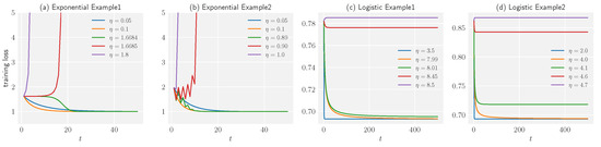
Consider optimizing $\mathcal{L}\left(w\right)$ with dataset $\{(x_1=1,y_1=1)\mathrm{and}(x_2=1,y_2=-1).\}$ using gradient descent with constant learning rates. Figure 2a,c shows the dependence of different dynamics on the learning rate η for exponential and logistic loss, respectively.

Figure 2. Showing the dependence of the dynamics of the training loss on the learning rate for linear predictors using both exponential and logistic loss functions. Examples 1 and 2 were used to test the performance of the linear predictors. The sub-graphs (a,c) show the experimental learning curves for separable data, consistent with the theoretical predictions. The critical learning rates were found to be ${\eta }_{\mathrm{critical}}=1.66843$ and ${\eta }_{\mathrm{critical}}=8.485$ for the exponential and logistic loss functions, respectively. Sub-graphs (b,d) show the dynamics of the training loss for non-separable data. The dynamics of training loss regarding the learning rate for non-separable data are similar to those of degenerate cases. Hence, the critical learning rates can be approximated by ${\eta }_{\mathrm{critical}}=0.895$ and ${\eta }_{\mathrm{critical}}=4.65$, respectively.

Example 2.

Consider optimizing $\mathcal{L}\left(w\right)$ with dataset $\{(x_1=1,y_1=1),(x_2=2,y_2=-1)\mathrm{and}$$(x_3=-1,y_3=1).\}$ using gradient descent with constant learning rates. Figure 2b,d shows the dependence of different dynamics on the learning rate η for exponential and logistic loss, respectively.

Remark 2.

The dataset considered here is an example of a non-separable case, and the dynamics of loss behave similarly to those in Example 1. We use this example to show that our theoretical results on the degenerate data can be extended empirically to the non-separable data.

4.2. Non-Convex Optimization

To investigate the relationship between the dynamics of gradient descent and the learning rate for deep linear networks, we consider linear networks with one hidden layer, and the information propagation in these networks is governed by,

$$f\left(x\right)=m^{-1/2}{w}^{\left(2\right)}{w}^{\left(1\right)}x,$$

(3)

where m is the width, i.e., the number of neurons in the hidden layer, $w^{\left(1\right)}\in {\mathbb{R}}^{m\times d}$ and $w^{\left(2\right)}\in {\mathbb{R}}^m$ are the parameters of the model. Taking the exponential loss as an example, the gradient descent equations at training step t are,

$$\begin{array}{cc}\hfill w_{t+1}^{\left(1\right)}& =w_t^{\left(1\right)}-\frac{1}{n}\frac{\eta }{m^{1/2}}(-e^{-y_{\alpha }{f}_t\left(x_{\alpha }\right)})w_t^{\left(2\right)}{x}_{\alpha }{y}_{\alpha },\hfill \\ \hfill w_{t+1}^{\left(2\right)}& =w_t^{\left(2\right)}-\frac{1}{n}\frac{\eta }{m^{1/2}}(-e^{-y_{\alpha }{f}_t\left(x_{\alpha }\right)})w_t^{\left(1\right)}{x}_{\alpha }{y}_{\alpha },\hfill \end{array}$$

(4)

where we use the Einstein summation convention to simplify the expression and apply this convention in the following derivation.

We introduce the neural tangent kernel, an essential element for the evolution of output function in Equation 8. The neural tangent kernel (NTK) originates from [1] and is formulated as,

$${\Theta }_{\alpha \beta }=\frac{1}{m}\sum _{p=1}^P\frac{\partial f\left(x_{\alpha }\right)}{{\partial }_{{\theta }_p}}\frac{\partial f\left(x_{\beta }\right)}{{\partial }_{{\theta }_p}}.$$

(5)

where P is the number of parameters. For a two-layer linear neural network, the NTK can be written as,

$${\Theta }_{\alpha \beta }=\frac{1}{mn}\left(\left(w^{\left(1\right)}{x}_{\alpha }\right)\left(w^{\left(1\right)}{x}_{\beta }\right)+{\left(w^{\left(2\right)}\right)}^2\left(x_{\alpha }{x}_{\beta }\right)\right).$$

(6)

Here we use normalized NTK which is divided by the number of samples n. Under the degeneracy Assumption 3, the loss function becomes $\mathcal{L}=cosh\left(m^{-1/2}{w}^{\left(2\right)}{w}^{\left(1\right)}\right)$. Then Equation (4) reduces to

$$\begin{array}{c}\hfill w_{t+1}^{\left(1\right)}=w_t^{\left(1\right)}-\frac{\eta }{m^{1/2}}{w}_t^{\left(2\right)}sinh\left(m^{-1/2}{w}_t^{\left(2\right)}{w}_t^{\left(1\right)}\right),\\ \hfill w_{t+1}^{\left(2\right)}=w_t^{\left(2\right)}-\frac{\eta }{m^{1/2}}{w}_t^{\left(1\right)}sinh\left(m^{-1/2}{w}_t^{\left(2\right)}{w}_t^{\left(1\right)}\right).\end{array}$$

(7)

The updates of output function $f_t$ and the eigenvalue of NTK ${\lambda }_t$, which are both scalars in our setting:

$$\begin{array}{cc}\hfill f_{t+1}& =f_t-\eta {\lambda }_t{\widetilde{f_t}}_{\exp }+\frac{{\eta }^2}{m}{f}_t{\widetilde{f_t^2}}_{\exp },\hfill \\ \hfill {\lambda }_{t+1}& ={\lambda }_t-\frac{4\eta }{m}{f}_t{\widetilde{f_t}}_{\exp }+\frac{{\eta }^2}{m}{\lambda }_t{\widetilde{f_t^2}}_{\exp }.\hfill \end{array}$$

(8)

where ${\widetilde{f_t}}_{\exp }:=sinh\left(f_t\right)$ while ${\widetilde{f_t}}_{\log }:=\frac{sinh\left(f_t\right)}{1+cosh\left(f_t\right)}$ for logistic loss.

We have previously introduced the catapult phase where the loss grows at the beginning and then drops until it converges to a global minimum. In the following theorem, we prove the existence of the catapult phase on the degenerate data with exponential and logistic loss.

Theorem 2.

Under appropriate initialization and Assumption 3, there exists a catapult phase for both the exponential and logistic loss. More precisely, when η belongs to this phase, $T>0$ exists such that the output function $f_t$ and the eigenvalue of NTK ${\lambda }_t$ update in the following way:

1. 

${\mathcal{L}}_t$ keeps increasing when $t<T$.

2. 

After the T step and its successors, the loss decreases, which is equivalent to:

$$|f_{T+1}|>|f_{T+2}|\ge |f_{T+3}|\ge \dots .$$

3. 

The eigenvalue of NTK keeps dropping after the T steps:

$${\lambda }_{T+1}>{\lambda }_{T+2}\ge {\lambda }_{T+3}\ge \dots .$$

Moreover, we have the inverse relationship between the learning rate and final eigenvalue of the NTK: ${\lambda }_{\infty }\le {lim}_{t\to \infty }\frac{4f_t}{\eta {\widetilde{f_t}}_{\exp }}$ with exponential loss, or ${\lambda }_{\infty }\le {lim}_{t\to \infty }\frac{4f_t}{\eta {\widetilde{f_t}}_{\log }}$ with logistic loss.

We demonstrate that the catapult phase can be found in both degenerate and non-separable data through the following examples. The weight matrix is initialized by iid Gaussian distribution, i.e., $w^{\left(1\right)},w^{\left(2\right)}\sim \mathcal{N}(0,{\sigma }_w^2)$. For exponential loss, we adopt the setting of ${\sigma }_w^2=0.5$ and $m=1000$ while we set ${\sigma }_w^2=1.0$ and $m=100$ for logistic loss.

Example 3.

Consider optimizing $\mathcal{L}\left(w\right)$ using a one-hidden-layer linear network with dataset $\{(x_1=[1,0],y_1=1)\mathrm{and}(x_2=[1,0],y_2=-1).\}$ and exponential (logistic) loss using gradient descent with a constant learning rate. Figure 1a,c,e,g shows how the different choices of learning rate η change the dynamics of the loss function with exponential and logistic loss.

Example 4.

Consider optimizing $\mathcal{L}\left(w\right)$ using a one-hidden-layer linear network with dataset $\{(x_1=[1,1],y_1=-1),(x_2=[1,-1],y_1=1),(x_3=[-1,-2],y_1=1)\mathrm{and}(x_4=[-1,1],y_4=1).\}$ and exponential (logistic) loss using gradient descent with a constant learning rate. Figure 1b,d,f,h shows how the different choices of learning rate η change the dynamics of the loss function with exponential and logistic loss.

As Figure 1 shows, in the catapult phase, the eigenvalue of the NTK decreases to a lower value than its initial point, while it remains unchanged in the lazy phase where the learning rate is small. For MSE loss, the lower value of the NTK indicates a flatter curvature given the training loss is low [16]. Yet, it is unknown whether the aforementioned conclusion can be applied to exponential and logistic loss. Through the following corollary, we show that the Hessian is equivalent to the NTK when the loss converges to a global minimum for degenerate data.

Corollary 1.

Consider optimizing $\mathcal{L}\left(w\right)$ with a one-hidden-layer linear network under Assumption 3 and exponential (logistic) loss using gradient descent with a constant learning rate. For any learning rate that loss can converge to the global minimum, the larger the learning rate, the flatter curvature the gradient descent will achieve at the end of training (see Corollary A1 in Appendix A for detail).

We demonstrate that the flatter curvature can be achieved in the catapult phase through Examples 3 and 4, using the code provided by [56] to measure the Hessian, as shown in Figure 3. In the lazy phase, both the curvature and eigenvalue of the NTK are independent of the learning rate at the end of training. In the catapult phase, however, the curvature decreases to a value smaller than that in the lazy phase. In conclusion, the NTK and Hessian have similar behaviours at the end of training on non-separable data.

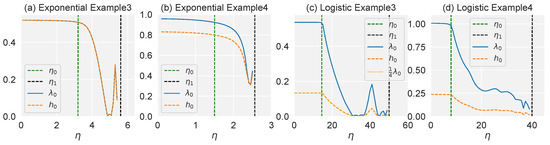
Figure 3. Top eigenvalue of the NTK (${\lambda }_0$) and Hessian ($h_0$) measured at $t=100$ as a function of the learning rate, with (a,b) exponential loss and (c,d) logistic loss in Examples 3 and 4. The green dashed line $\eta ={\eta }_0$ represents the boundary between the lazy and catapult phases, while the black dashed line $\eta ={\eta }_1$ separates the catapult and divergent phases. We adopt the settings of ${\sigma }_w^2=0.5$ and $m=100$ for exponential loss, and the settings for logistic loss are ${\sigma }_w^2=0.5$ and $m=200$. (a,c) The curves of the maximum eigenvalue of the NTK and Hessian coincide as predicted by the Corollary A1. (b,d) For non-separable data, the trend of the two eigenvalue curves is consistent with the change in the learning rate.

Finally, we compare our results from the catapult phase to the results with MSE loss and show the summary in Table 2.

Table 2. A summary of the relationship between separation conditions of the data and the catapult phase for different losses.

Separation Condition	Linear Separable	Degenerate	Non-Separable
Exponential loss (this work)	✗	✓	✓
Logistic loss (this work)	✗	✓	✓
Squared loss ([16])	✓	✓	✓

5. Experiment

5.1. Experimental Results

In this section, we present our experimental results of linear networks with the logistic loss on CIFAR-10 to examine whether flatter minima achieved in the catapult phase can lead to better generalization in real applications. We selected two (“cars” and “dogs”) of the ten categories from the CIFAR-10 dataset to form a binary classification problem. Training is performed on a server with a CPU with 32 cores, and an 8 GB Nvidia 3060 GPU. The results will be illustrated by comparing the generalization performance with respect to different learning rates.

Figure 4 shows the performance of the two linear networks, one has one hidden layer without bias, and the other has two hidden layers of linear network with bias, trained on CIFAR-10. We present the results using two different stopping conditions. Firstly, we fix the training time for all learning rates, the learning rates within the catapult phase have the advantage of obtaining a higher test accuracy, as shown in Figure 4a,c. However, adopting a fixed training time will result in a bias in favour of large learning rates, since the large learning rate naturally runs faster. To ensure a fair comparison, we then used a fixed physical time, defined as $t_{\mathrm{phy}}=t_0\eta$, where $t_0$ is a constant. In this setting, as shown in Figure 4b,d, the performance of the large learning rate phase is even worse than that of the small learning phase. Nevertheless, we find this is achieved in the catapult phase when adopting the learning rate annealing strategy.

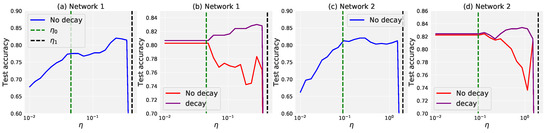
Figure 4. Test performance on the CIFAR-10 dataset with respect to different learning rate phases. The data size is of $n_{\mathrm{train}}=2048$ and $n_{\mathrm{test}}=512$. (a,b) A two-layer linear network without bias of ${\sigma }_w^2=0.5$ and $m=500$. (c,d) A three-layer linear network with the bias of ${\sigma }_w^2=0.5$, ${\sigma }_b^2=0.01$, and $m=500$. (a,c) The test accuracy is measured at the time step $t=500$ and $t=300$, respectively. The optimal performance is obtained when the learning rate is in the catapult phase. (b,d) The test accuracy is measured at the physical time step (red curve), after which it continues to evolve for a period of time at a small learning rate (purple): $t_{\mathrm{phy}}=50/\eta$ and extra time $t=500$ at $\eta =0.01$ for the decaying case. Although the results in the catapult phase do not perform as well as the lazy phase when there is no decay, the best performance can be found in the catapult phase when adopting learning rate annealing.

To explain the above experimental results, we refer to Theorem 2 in [30]. According to this theorem, the data can be uniquely partitioned into the linearly separable and non-separable parts. When we tune the learning rate to the large learning rate regime, the algorithm quickly iterates to a flat minimum in a space spanned by non-separable data. At the same time, for linearly separable data, the gradient descent cannot achieve the maximum margin due to the large learning rate. As a result, for this part of the data, the generalization performance is suppressed. This explains why when we fix the physical steps, the performance in the large learning rate regime is worse than that of the small learning rate phase. On the other hand, when we adopt the strategy of learning rate annealing, for non-separable data, since the large learning rate has learned a flat curvature, the subsequent small learning rate will not affect this result. For data with linearly separable parts, reducing the learning rate can restore the maximum margin. Therefore, we can see that under this strategy, the best performance can be found in the phase of a large learning rate.

5.2. Effectiveness on Synthetic and Real-World Datasets

To further evaluate the impact of learning rate annealing strategies on model performance, we conducted experiments using two different annealing strategies powered by the learning rate scheduler in PyTorch: one-step annealing and exponential annealing. In the one-step annealing strategy, we started with a relatively large learning rate of 1 and then reduced it by a decay factor of 0.01 after 30 training steps. In the exponential annealing strategy, we started with a large learning rate of 1 and then reduced it exponentially with a learning rate decay rate of 0.98 over time. We evaluated the performance of these two annealing strategies on both synthetic and real-world datasets using convolutional neural networks. Specifically, we measured the accuracy of the models trained with each annealing strategy.

Creating synthetic data with label noise can help represent the separability of the data by simulating a more realistic scenario in which data points may not be perfectly separable. We synthesize the label noise on three public datasets MNIST, CIFAR-10 and CIFAR-100 following previous works [57,58,59]. Symmetric noise was generated by randomly flipping the labels of each class to incorrect labels from other classes. Asymmetric noise was generated by flipping the labels within a specific set of classes to a certain incorrect class. For example, for CIFAR-10, flipping “truck” → “automobile”, “bird” → “airplane”, “deer” → “horse”, “cat” ↔ “dog”. In CIFAR-100, the 100 classes were grouped into 20 super-classes, each with 5 sub-classes, and each class was flipped to the next class in a circular fashion within the same super-class. The noise rate $\tau \in [0.1,0.4]$ for both symmetric and asymmetric noise. Regarding the models a four-layer CNN for MNIST, an eight-layer CNN for CIFAR-10 and a ResNet-34 for CIFAR-100. We train the networks for 50, 120 and 200 epochs for MNIST, CIFAR-10, and CIFAR-100, respectively. For all training, we used a SGD optimizer with no momentum, cross-entropy loss, and three different learning rate schedules. Typical data augmentations including random width/height shift and horizontal flip were applied.

The classification accuracies under symmetric label noise are reported in Table 3. As can be seen, the learning rate annealing methods achieved better results across all datasets. The superior performance of the learning rate annealing methods is more pronounced when the noise rates are extremely high and the dataset is more complex. Results for asymmetric noise are reported in Table 4. Comparing the results in both Table 3 and Table 4, we find that learning rate annealing is quite consistent across different noise types and rates. Overall, this demonstrates a consistently strong performance across different datasets.

Table 3. Test accuracy (%) of different methods on benchmark datasets with clean or symmetric label noise ($\tau \in [0.1,0.4]$). The results (mean ± std) are reported over three random runs. SL refers to a training schedule with a small learning rate that remains constant throughout the training process. OS (one-step) denotes a training schedule where the learning rate starts at a high value and then drops to a smaller value after a specified number of training steps. Exp refers to a training schedule where the learning rate decreases exponentially as the training progresses.

Datasets	Methods	Clean $\mathbf{(}\mathit{\tau }=\mathbf{0.0}\mathbf{)}$	Symmetric Noise Rate ($\mathit{\tau }$)
			0.1	0.2	0.3	0.4
MNIST	SL	$99.09\pm 0.02$	$98.60\pm 0.04$	$98.29\pm 0.08$	$97.88\pm 0.12$	$97.57\pm 0.09$
	OS	$99.33\pm 0.04$	$99.22\pm 0.57$	$98.71\pm 0.10$	$98.34\pm 0.07$	$97.96\pm 0.16$
	EXP	$99.40\pm 0.03$	$98.85\pm 0.21$	$98.84\pm 0.10$	$98.63\pm 0.20$	$98.48\pm 0.03$
CIFAR-10	SL	$86.37\pm 0.05$	$82.01\pm 0.19$	$78.70\pm 0.29$	$75.83\pm 0.28$	$71.58\pm 0.08$
	OS	$91.38\pm 0.07$	$86.87\pm 0.15$	$83.95\pm 0.24$	$81.72\pm 0.08$	$78.70\pm 0.25$
	EXP	$91.63\pm 0.15$	$85.52\pm 0.22$	$82.94\pm 0.32$	$81.57\pm 0.99$	$79.66\pm 2.20$
CIFAR-100	SL	$48.10\pm 0.14$	$42.31\pm 0.44$	$38.10\pm 0.65$	$34.10\pm 0.25$	$31.21\pm 1.01$
	OS	$70.50\pm 1.07$	$62.66\pm 1.51$	$57.31\pm 2.09$	$52.08\pm 1.63$	$47.22\pm 0.88$
	EXP	$70.14\pm 0.82$	$63.67\pm 0.26$	$55.70\pm 0.24$	$49.67\pm 1.95$	$43.39\pm 1.11$

Table 4. Test accuracy (%) of different methods on benchmark datasets with clean or asymmetric label noise ($\tau \in [0.1,0.4]$). The results (mean ± std) are reported over three random runs. SL refers to a training schedule with a small learning rate that remains constant throughout the training process. OS (one-step) denotes a training schedule where the learning rate starts at a high value and then drops to a smaller value after a specified number of training steps. Exp refers to a training schedule where the learning rate decreases exponentially as the training progresses.

Datasets	Methods	Clean $\mathbf{(}\mathit{\tau }=\mathbf{0.0}\mathbf{)}$	Asymmetric Noise Rate ($\mathit{\tau }$)
			0.1	0.2	0.3	0.4
MNIST	SL	$99.09\pm 0.02$	$98.52\pm 0.07$	$98.25\pm 0.01$	$97.89\pm 0.16$	$97.45\pm 0.01$
	OS	$99.33\pm 0.04$	$98.86\pm 0.16$	$98.98\pm 0.71$	$98.35\pm 0.14$	$98.24\pm 0.17$
	EXP	$99.40\pm 0.03$	$98.85\pm 0.09$	$98.63\pm 0.09$	$98.46\pm 0.13$	$98.24\pm 0.15$
CIFAR-10	SL	$86.37\pm 0.05$	$81.91\pm 0.25$	$78.87\pm 0.11$	$75.85\pm 0.17$	$72.02\pm 0.59$
	OS	$91.38\pm 0.07$	$86.61\pm 0.32$	$83.90\pm 0.41$	$81.41\pm 0.41$	$78.77\pm 0.40$
	EXP	$91.63\pm 0.15$	$85.26\pm 0.79$	$83.53\pm 0.37$	$81.38\pm 1.05$	$78.82\pm 0.45$
CIFAR-100	SL	$48.10\pm 0.14$	$42.15\pm 0.13$	$37.93\pm 0.95$	$34.80\pm 0.28$	$30.97\pm 0.54$
	OS	$70.50\pm 1.07$	$62.65\pm 0.91$	$57.66\pm 0.97$	$50.42\pm 1.06$	$47.07\pm 1.74$
	EXP	$70.14\pm 0.82$	$63.51\pm 1.20$	$56.35\pm 0.55$	$48.09\pm 0.44$	$44.34\pm 0.40$

To further enhance our theoretical finding and complement the effectiveness of the general annealing methods, we conducted experiments on the large-scale real-world dataset WebVision [25] as it is a large-scale dataset of images that has been specifically designed to evaluate the performance of computer vision algorithms under noise. We followed the “Mini” setting in [24,59] that only takes the first 50 classes of the resized Google image subset. We evaluated the trained networks on the same 50 classes of the WebVision validation set, considered as a clean validation.

We trained a ResNet-50 [14] using SGD for 250 epochs with a Nesterov momentum of 0.9, a weight decay of $3\times {10}^{-5}$, and a batch size of 512. We resized the images to $224\times 224$. Typical data augmentations, including random width/height shift, colour jittering and random horizontal flip, were applied. The accuracies on the clean WebVision validation set (e.g., only the first 50 classes) are reported in Table 5. As a result, the large learning rate annealing methods (one-step annealing and exponential learning rate annealing) provided better generalization.

Table 5. Test accuracies (%) on the clean WebVision validation set of ResNet-50 models trained on WebVision. SL refers to a training schedule with a small learning rate that remains constant throughout the training process. OS (one-step) denotes a training schedule where the learning rate starts at a high value and then drops to a smaller value after a specified number of training steps. Exp refers to a training schedule where the learning rate decreases exponentially as the training progresses.

Loss	SL	OS	EXP
Acc	60.38	66.04	65.92

In terms of computational complexity, the actual process of changing the magnitude of the learning rate during training is typically straightforward and computationally inexpensive. The real computational cost of learning rate annealing comes from the additional training iterations required to allow the model to converge more precisely towards the optimal solution. Overall, the actual computational cost of learning rate annealing can depend on a variety of factors, including the size of the dataset, the complexity of the model, and the specific annealing schedule used. However, in general, the computational cost of learning rate annealing is relatively small compared to the overall cost of training a deep learning model.

6. Discussion

In this work, we characterized the dynamics of deep linear networks for binary classification trained with gradient descent in a large learning rate regime, inspired by the seminal work by [16]. We present a catapult effect in the large learning rate phase depending on separation conditions associated with logistic and exponential loss. According to our theoretical analysis, the loss in the catapult phase can converge to the global minimum like the lazy phase. However, from the perspective of the Hessian, the minimum achieved in the catapult phase is flatter. We empirically show that even without SGD optimization, the best generalization performance can be achieved in the catapult stage phase for linear networks, while this works in the large learning rate for linear networks in binary classification, there are several remaining open questions. For non-linear networks, the effect of a large learning rate is not clear in theory. In addition, the stochastic gradient descent algorithm also needs to be explored when the learning rate is large. We leave these unsolved problems for future work.

Future work could investigate the theoretical impact of data separability on a wider range of deep learning models, including convolutional neural networks or recurrent neural networks, and for different types of loss functions. Additionally, it would be beneficial to explore the effect of data separability on the design of neural network architectures, such as varying the number of layers, hidden unit size, or connectivity patterns. Furthermore, our study assumes degenerate data, which simplifies the analysis. As new mathematical analytical methods become available, future research could extend the results to non-degenerate datasets and explore how the relationship between data separability and training dynamics/model performance changes in this setting. Finally, practical applications of this research could be explored, such as utilizing data separability to guide the design of neural networks or the development of learning rate annealing schemes.

References

- Jacot, A.; Gabriel, F.; Hongler, C. Neural tangent kernel: Convergence and generalization in neural networks. In Proceedings of the Advances in Neural Information Processing Systems, Red Hook, NY, USA, 3–8 December 2018; pp. 8571–8580. [Google Scholar]
- Allen-Zhu, Z.; Li, Y.; Song, Z. A convergence theory for deep learning via over-parameterization. In Proceedings of the International Conference on Machine Learning. PMLR, Long Beach, CA, USA, 9–15 June 2019; pp. 242–252. [Google Scholar]
- Du, S.S.; Lee, J.D.; Li, H.; Wang, L.; Zhai, X. Gradient descent finds global minima of deep neural networks. arXiv 2018, arXiv:1811.03804. [Google Scholar]
- Chizat, L.; Bach, F. On the global convergence of gradient descent for over-parameterized models using optimal transport. In Proceedings of the Advances in Neural Information Processing Systems, Red Hook, NY, USA, 3–8 December 2018; pp. 3036–3046. [Google Scholar]
- Zou, D.; Cao, Y.; Zhou, D.; Gu, Q. Stochastic gradient descent optimizes over-parameterized deep ReLU networks. arXiv 2018, arXiv:1811.08888. [Google Scholar]
- Huang, W.; Liu, C.; Chen, Y.; Liu, T.; Da Xu, R.Y. Demystify Optimization and Generalization of Over-parameterized PAC-Bayesian Learning. arXiv 2022, arXiv:2202.01958. [Google Scholar]
- Nakkiran, P.; Kaplun, G.; Bansal, Y.; Yang, T.; Barak, B.; Sutskever, I. Deep double descent: Where bigger models and more data hurt. arXiv 2019, arXiv:1912.02292. [Google Scholar] [CrossRef]
- Soudry, D.; Hoffer, E.; Nacson, M.S.; Gunasekar, S.; Srebro, N. The implicit bias of gradient descent on separable data. J. Mach. Learn. Res. 2018, 19, 2822–2878. [Google Scholar]
- Neyshabur, B.; Tomioka, R.; Srebro, N. In search of the real inductive bias: On the role of implicit regularization in deep learning. arXiv 2014, arXiv:1412.6614. [Google Scholar]
- Gunasekar, S.; Lee, J.; Soudry, D.; Srebro, N. Characterizing implicit bias in terms of optimization geometry. arXiv 2018, arXiv:1802.08246. [Google Scholar]
- Ji, Z.; Telgarsky, M. The implicit bias of gradient descent on nonseparable data. In Proceedings of the Conference on Learning Theory, Phoenix, AZ, USA, 25–28 June 2019; pp. 1772–1798. [Google Scholar]
- Nacson, M.S.; Gunasekar, S.; Lee, J.D.; Srebro, N.; Soudry, D. Lexicographic and depth-sensitive margins in homogeneous and non-homogeneous deep models. arXiv 2019, arXiv:1905.07325. [Google Scholar]
- Lyu, K.; Li, J. Gradient descent maximizes the margin of homogeneous neural networks. arXiv 2019, arXiv:1906.05890. [Google Scholar]
- He, K.; Zhang, X.; Ren, S.; Sun, J. Deep residual learning for image recognition. In Proceedings of the IEEE Conference on Computer Vision and Pattern Recognition, Las Vegas, NV, USA, 26 June–1 July 2016; pp. 770–778. [Google Scholar]
- Zagoruyko, S.; Komodakis, N. Wide residual networks. arXiv 2016, arXiv:1605.07146. [Google Scholar]
- Lewkowycz, A.; Bahri, Y.; Dyer, E.; Sohl-Dickstein, J.; Gur-Ari, G. The large learning rate phase of deep learning: The catapult mechanism. arXiv 2020, arXiv:2003.02218. [Google Scholar]
- Arora, S.; Du, S.S.; Hu, W.; Li, Z.; Salakhutdinov, R.R.; Wang, R. On exact computation with an infinitely wide neural net. In Proceedings of the Advances in Neural Information Processing Systems, Vancouver, BC, Canada, 8–14 December 2019; pp. 8141–8150. [Google Scholar]
- Yang, G. Scaling limits of wide neural networks with weight sharing: Gaussian process behavior, gradient independence, and neural tangent kernel derivation. arXiv 2019, arXiv:1902.04760. [Google Scholar]
- Huang, J.; Yau, H.T. Dynamics of deep neural networks and neural tangent hierarchy. arXiv 2019, arXiv:1909.08156. [Google Scholar]
- Allen-Zhu, Z.; Li, Y. What Can ResNet Learn Efficiently, Going Beyond Kernels? In Proceedings of the Advances in Neural Information Processing Systems, Vancouver, BC, Canada, 8–14 December2019; pp. 9017–9028. [Google Scholar]
- Chizat, L.; Oyallon, E.; Bach, F. On lazy training in differentiable programming. In Proceedings of the Advances in Neural Information Processing Systems, Vancouver, BC, Canada, 8–14 December2019; pp. 2937–2947. [Google Scholar]
- Cohen, G.; Afshar, S.; Tapson, J.; Van Schaik, A. EMNIST: Extending MNIST to handwritten letters. In Proceedings of the 2017 international joint conference on neural networks (IJCNN), Anchorage, AK, USA, 14–19 May 2017; pp. 2921–2926. [Google Scholar]
- Ho-Phuoc, T. CIFAR10 to compare visual recognition performance between deep neural networks and humans. arXiv 2018, arXiv:1811.07270. [Google Scholar]
- Jiang, L.; Zhou, Z.; Leung, T.; Li, L.J.; Fei-Fei, L. MentorNet: Learning Data-Driven Curriculum for Very Deep Neural Networks on Corrupted Labels. In Proceedings of the ICML, Stockholm, Sweden, 10–15 July 2018. [Google Scholar]
- Li, W.; Wang, L.; Li, W.; Agustsson, E.; Van Gool, L. Webvision database: Visual learning and understanding from web data. arXiv 2017, arXiv:1708.02862. [Google Scholar]
- Ali, A.; Dobriban, E.; Tibshirani, R.J. The Implicit Regularization of Stochastic Gradient Flow for Least Squares. arXiv 2020, arXiv:2003.07802. [Google Scholar]
- Mousavi-Hosseini, A.; Park, S.; Girotti, M.; Mitliagkas, I.; Erdogdu, M.A. Neural Networks Efficiently Learn Low-Dimensional Representations with SGD. arXiv 2022, arXiv:2209.14863. [Google Scholar]
- Nacson, M.S.; Lee, J.D.; Gunasekar, S.; Savarese, P.H.; Srebro, N.; Soudry, D. Convergence of gradient descent on separable data. arXiv 2018, arXiv:1803.01905. [Google Scholar]
- Gunasekar, S.; Lee, J.D.; Soudry, D.; Srebro, N. Implicit bias of gradient descent on linear convolutional networks. In Proceedings of the Advances in Neural Information Processing Systems, Red Hook, NY, USA, 3–8 December 2018; pp. 9461–9471. [Google Scholar]
- Ji, Z.; Telgarsky, M. Gradient descent aligns the layers of deep linear networks. arXiv 2018, arXiv:1810.02032. [Google Scholar]
- Razin, N.; Cohen, N. Implicit Regularization in Deep Learning May Not Be Explainable by Norms. arXiv 2020, arXiv:2005.06398. [Google Scholar]
- Smith, S.L.; Dherin, B.; Barrett, D.G.; De, S. On the origin of implicit regularization in stochastic gradient descent. arXiv 2021, arXiv:2101.12176. [Google Scholar]
- Ji, Z.; Telgarsky, M. Directional convergence and alignment in deep learning. arXiv 2020, arXiv:2006.06657. [Google Scholar]
- Chizat, L.; Bach, F. Implicit bias of gradient descent for wide two-layer neural networks trained with the logistic loss. arXiv 2020, arXiv:2002.04486. [Google Scholar]
- Oymak, S.; Soltanolkotabi, M. Overparameterized nonlinear learning: Gradient descent takes the shortest path? arXiv 2018, arXiv:1812.10004. [Google Scholar]
- Nguyen, T.; Novak, R.; Xiao, L.; Lee, J. Dataset distillation with infinitely wide convolutional networks. Adv. Neural Inf. Process. Syst. 2021, 34, 5186–5198. [Google Scholar]
- Ho, T.K.; Basu, M. Complexity measures of supervised classification problems. IEEE Trans. Pattern Anal. Mach. Intell. 2002, 24, 289–300. [Google Scholar]
- Lorena, A.C.; Garcia, L.P.; Lehmann, J.; Souto, M.C.; Ho, T.K. How complex is your classification problem? a survey on measuring classification complexity. ACM Comput. Surv. (CSUR) 2019, 52, 1–34. [Google Scholar] [CrossRef]
- Guan, S.; Loew, M.; Ko, H. Data separability for neural network classifiers and the development of a separability index. arXiv 2020, arXiv:2005.13120. [Google Scholar]
- Rostami, M.; Berahmand, K.; Nasiri, E.; Forouzandeh, S. Review of swarm intelligence-based feature selection methods. Eng. Appl. Artif. Intell. 2021, 100, 104210. [Google Scholar] [CrossRef]
- Berahmand, K.; Mohammadi, M.; Saberi-Movahed, F.; Li, Y.; Xu, Y. Graph regularized nonnegative matrix factorization for community detection in attributed networks. IEEE Trans. Netw. Sci. Eng. 2022, 10, 372–385. [Google Scholar] [CrossRef]
- Bietti, A.; Bruna, J.; Sanford, C.; Song, M.J. Learning Single-Index Models with Shallow Neural Networks. arXiv 2022, arXiv:2210.15651. [Google Scholar]
- Lee, J.; Xiao, L.; Schoenholz, S.; Bahri, Y.; Novak, R.; Sohl-Dickstein, J.; Pennington, J. Wide neural networks of any depth evolve as linear models under gradient descent. In Proceedings of the Advances in Neural Information Processing Systems, Vancouver, BC, Canada, 8–14 December 2019; pp. 8570–8581. [Google Scholar]
- Huang, W.; Du, W.; Da Xu, R.Y. On the Neural Tangent Kernel of Deep Networks with Orthogonal Initialization. arXiv 2020, arXiv:2004.05867. [Google Scholar]
- Li, Z.; Wang, R.; Yu, D.; Du, S.S.; Hu, W.; Salakhutdinov, R.; Arora, S. Enhanced convolutional neural tangent kernels. arXiv 2019, arXiv:1911.00809. [Google Scholar]
- Du, S.S.; Hou, K.; Salakhutdinov, R.R.; Poczos, B.; Wang, R.; Xu, K. Graph neural tangent kernel: Fusing graph neural networks with graph kernels. In Proceedings of the Advances in Neural Information Processing Systems, Vancouver, BC, Canada, 8–14 December 2019; pp. 5723–5733. [Google Scholar]
- Huang, W.; Li, Y.; Du, W.; Yin, J.; Da Xu, R.Y.; Chen, L.; Zhang, M. Towards deepening graph neural networks: A GNTK-based optimization perspective. arXiv 2021, arXiv:2103.03113. [Google Scholar]
- Hron, J.; Bahri, Y.; Sohl-Dickstein, J.; Novak, R. Infinite attention: NNGP and NTK for deep attention networks. arXiv 2020, arXiv:2006.10540. [Google Scholar]
- Jacot, A.; Gabriel, F.; Hongler, C. Freeze and chaos for dnns: An NTK view of batch normalization, checkerboard and boundary effects. arXiv 2019, arXiv:1907.05715. [Google Scholar]
- Yang, G. Tensor Programs II: Neural Tangent Kernel for Any Architecture. arXiv 2020, arXiv:2006.14548. [Google Scholar]
- Krizhevsky, A.; Sutskever, I.; Hinton, G.E. Imagenet classification with deep convolutional neural networks. In Proceedings of the Advances in neural information processing systems, Lake Tahoe, NV, USA, 3–6 December 2012; pp. 1097–1105. [Google Scholar]
- Keskar, N.S.; Mudigere, D.; Nocedal, J.; Smelyanskiy, M.; Tang, P.T.P. On large-batch training for deep learning: Generalization gap and sharp minima. arXiv 2016, arXiv:1609.04836. [Google Scholar]
- Jiang, Y.; Neyshabur, B.; Mobahi, H.; Krishnan, D.; Bengio, S. Fantastic generalization measures and where to find them. arXiv 2019, arXiv:1912.02178. [Google Scholar]
- Li, Y.; Wei, C.; Ma, T. Towards explaining the regularization effect of initial large learning rate in training neural networks. In Proceedings of the Advances in Neural Information Processing Systems, Vancouver, BC, Canada, 8–14 December 2019; pp. 11674–11685. [Google Scholar]
- Nitanda, A.; Chinot, G.; Suzuki, T. Gradient Descent can Learn Less Over-parameterized Two-layer Neural Networks on Classification Problems. arXiv 2019, arXiv:1905.09870. [Google Scholar]
- Nilsen, G.K.; Munthe-Kaas, A.Z.; Skaug, H.J.; Brun, M. Efficient computation of hessian matrices in tensorflow. arXiv 2019, arXiv:1905.05559. [Google Scholar]
- Patrini, G.; Rozza, A.; Krishna Menon, A.; Nock, R.; Qu, L. Making deep neural networks robust to label noise: A loss correction approach. In Proceedings of the IEEE Conference on Computer Vision and Pattern Recognition, Honolulu, HI, USA, 21–26 July 2017; pp. 1944–1952. [Google Scholar]
- Ma, X.; Wang, Y.; Houle, M.E.; Zhou, S.; Erfani, S.M.; Xia, S.T.; Wijewickrema, S.; Bailey, J. Dimensionality-Driven Learning with Noisy Labels. In Proceedings of the ICML, Stockholm, Sweden, 10–15 July 2018. [Google Scholar]
- Ma, X.; Huang, H.; Wang, Y.; Romano, S.; Erfani, S.; Bailey, J. Normalized loss functions for deep learning with noisy labels. In Proceedings of the International Conference on Machine Learning, Atlanta, GA, USA, 16–21 June 2013; PMLR: New York, NY, USA, 2020; pp. 6543–6553. [Google Scholar]
- Bubeck, S. Convex optimization: Algorithms and complexity. arXiv 2014, arXiv:1405.4980. [Google Scholar]
Disclaimer/Publisher’s Note: The statements, opinions and data contained in all publications are solely those of the individual author(s) and contributor(s) and not of MDPI and/or the editor(s). MDPI and/or the editor(s) disclaim responsibility for any injury to people or property resulting from any ideas, methods, instructions or products referred to in the content. |
© 2023 by the authors. Licensee MDPI, Basel, Switzerland. This article is an open access article distributed under the terms and conditions of the Creative Commons Attribution (CC BY) license (https://creativecommons.org/licenses/by/4.0/).