Short Landing for Flying-Wing Unmanned Aircraft with Thrust Vector

Abstract

The task of achieving a safe and short landing for a flying-wing unmanned aircraft with a three-bearing-swivel thrust vector is highly challenging. The process is further complicated due to the need to switch between multiple control modes, while also ensuring the protection of the flight boundaries from environmental disturbances and model uncertainties to ensure flight safety. To address this challenge, this paper proposes a short-landing strategy that employs mixed control using lift fans, thrust vectors, and aerodynamic control surfaces. The extended state observer (ESO) is integrated into the inner angular rate control and outer sink rate control to account for environmental disturbances and model uncertainties. To ensure flight safety, the attainable linear and angular acceleration is calculated through a trim analysis to determine the command value of velocity and angle of attack during a short landing. Additionally, a flight boundary protection method is employed which includes an additional command value of the angle of attack, resulting in a higher probability of a successful landing. This paper provides a detailed description of the short-landing strategy, including the control objectives for each phase. Finally, a Monte Carlo simulation is conducted to evaluate the effectiveness and robustness of the short-landing strategy, and the landing accuracy is assessed using the circular error probability metric.

1. Introduction

The rapid development of unmanned aerial vehicles (UAVs) and thrust vector control technologies has opened up new possibilities for automatic landing operations, including vertical landing, shipborne rolling vertical landing (SRVL), and short-landing techniques. Among these, the short landing has gained popularity, as it reduces runway reliance by lowering the touch-down speed and enhances the aircraft’s bring-back capability. However, the application of thrust vector control to short landings poses significant challenges.

First, the landing process requires careful consideration of the trim problem that arises from balancing the aerodynamic and direct forces generated by the thrust vector. Second, a proper control allocation strategy must be developed to account for the varying dynamic responses of the actuators involved. Third, a unified control framework that can adapt to control-mode switching is crucial for simplifying the controller design. Fourth, the control objects for each landing phase must be defined to ensure smooth operation. Finally, the control system must be robust to model uncertainties during the short-landing process. Addressing these challenges is critical to ensure the safety of short landings with thrust vector control. By fully considering the above five points, a well-designed control system can facilitate the successful execution of short-landing techniques, bringing new possibilities and benefits to UAV operations.

Thrust vector control has been extensively researched, with several notable advancements. Integrated thrust-vector (ITV) control technology has been widely used in post-stall envelope expansion by implementing the engine nozzle [1]. In history, there have been attempts to apply thrust vectoring for the takeoff and landing of the Harrier aircraft [2,3]. The Lianistry of Defence has led the development of shipborne rolling vertical landing (SRVL) technology for F-35B carrier aircraft landing, and thrust vector control has been applied to improve the performance of a damaged fighter [4]. The F-35B is well-known for its short takeoff and vertical landing (STVL) capabilities [5], which are supported by thrust vectoring technology. Additionally, the UK Ministry of Defence [6,7] has improved the payload performance of weapons—as this was previously a weak point for vertical landings—through the use of thrust vectoring. On 13 October 2018, British pilot Peter Wilson successfully completed the first SRVL flight [8], landing the F-35B 755 feet above HMS Queen Elizabeth’s ski-jump deck, and then taxied 175 feet before using the aircraft’s brakes to bring it to a standstill from 40 knots. Compared to vertical landing, SRVL lands at a slow forward speed and uses wing lift to supplement the propulsion system. Reference [9] developed the optimal trajectory transition controller for a thrust-vectored V/STOL aircraft. In Reference [10], the problem of the short takeoff curve was solved with the optimal tilt angle optimization. Different from the straight-line approach [11,12] taken by the F-35B in SRVL, Nicolas et al. [13] used a curved approach with a fixed-wing UAV and evaluated the predefined spline path, using flight tests. Furthermore, fast transition maneuvers along curved trajectories can reduce landing times [14].

Flying-wing unmanned aircraft, with their blended wing body layout [15], have a high lift-to-drag ratio but suffer from bad static heading stability [16] and control coupling, posing a significant threat to flight safety. To address this, Wang et al. [17] used the eigenstructure assignment (EA) method to realize three-axis decoupled control, which considers flying quality specifications during the control law design process. In addition, nonlinear dynamic inversion control (NDI) is utilized to deal with nonlinear coupling dynamics, as X-35B did [18]. However, these model-dependent design approach produce an unsatisfying result in the presence of model uncertainties. Therefore, robust control [19], incremental nonlinear dynamic inversion (INDI) control [20,21], and adaptive control [22] have been applied to improve the robustness of modeling uncertainties. Among these, active disturbance rejection control (ADRC) [23,24] uses disturbance-observer-based control, treating model uncertainties and environmental disturbances as lumped disturbances. An extended state observer (ESO) is designed to estimate and compensate for the lumped disturbance, showing excellent robustness.

The present study proposes a short-landing strategy utilizing thrust vector control, which features a continuous curved landing approach. To begin with, a detailed aircraft dynamics model is developed for landing simulation and performance analysis. To enhance the safety of the landing process, the attainable area of the linear and angular acceleration is determined based on the trim calculation to determine the reference values for the angle of attack and velocity during the short landing. Subsequently, a three-axis decoupled control law is designed using an extended state observer (ESO). The ESO is used to estimate and compensate for lumped disturbances, thus ensuring robustness against modeling uncertainties. To address the switching between different control modes during the landing process, the angular rate is selected as the control object of the inner loop, and the angular acceleration commands are allocated based on the different dynamics of the actuators. Furthermore, an overall control structure with multimode control is proposed which clarifies the control objectives for each phase of the landing process. Additionally, a flight-regime protection method is introduced to enhance landing safety by incorporating an additional angle of attack-command compensation. Finally, a nominal simulation and a Monte Carlo simulation are performed to assess the effectiveness and robustness of the proposed control strategy. The former involves a simulation without model parameters’ perturbation, while the latter assesses the robustness of the control strategy against modeling uncertainties.

This paper is organized as follows: Section 2 provides a detailed description of the configuration of the flying-wing UAV, and a dynamic model is developed to analyze the aircraft’s behavior during the short-landing process. Section 3 presents the trim analysis results and defines the equilibrium points for the reference angle of attack and velocity, which are critical parameters for ensuring safe and efficient short landing. Section 4 comprehensively elaborates on the design of the control system, including the various control loops, allocation of control commands, and the overall control structure. In Section 5, a novel short-landing strategy incorporating lateral and vertical guidance is proposed. The effectiveness of the proposed strategy is evaluated through numerical simulations, which are presented in Section 6. Finally, in Section 7, the main findings of the paper are summarized, and conclusions are drawn.

2. Aircraft Dynamics Model

2.1. Configuration Description

Figure 1 depicts the flying-wing UAV that was utilized in this study. The UAV is equipped with two lift fans and a thrust vector mechanism for pitch and yaw control. The lift fans, which are powered by Li-Po batteries, are positioned at a fixed angle at the front of the fuselage. The thrust vector mechanism, consisting of a turbojet engine and a 3BSD nozzle, is similar to that used in the F-35B [5]. The thrust-to-weight ratio of the UAV, despite having two lift fans, is approximately 0.69. Although the UAV is unable to perform vertical landing as the F-35B does [25], it can accomplish short takeoff and short landing (STOSL) by using its lift fans and vectored thrust. The nozzle pitch angle ranges from 0 to 90°, while the yaw angle ranges from −15 to 15°. The use of vectored thrust is restricted to the takeoff and landing phases, thus resulting in an improved takeoff and landing performance. During cruise flight, the nozzle remains level, and the rear engine door is shut, allowing the UAV to function as a standard flying-wing aircraft.

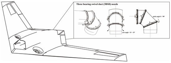
Figure 1. General diagram of the configuration of the subject flyingwing UAV.

Figure 2 displays the aerodynamic control surfaces utilized in this study; they consist of four elevons for controlling pitch and roll, segmented into elevators and ailerons. In addition, two spoiler-slot deflectors (SSDs) are employed to govern yaw motion. Relevant aircraft parameters are concisely summarized in Table 1.

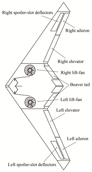
Figure 2. Top view of the flying-wing UAV.

Table 1. Physical parameters of the target aircraft.

Parameter	Explanation	Value
m	Mass	62 kg
S	Wing area	1.8 m2
b	Wingspan	3.2 m
Tv max	Maximum thrust of the turbojet engine	270 N
Tf max	Maximum force per lift fan	75 N
Ixx	Moment of inertia around body x-axis	72.1 kg·m2
Iyy	Moment of inertia around body y-axis	63.7 kg·m2
Izz	Moment of inertia around body z-axis	112.3 kg·m2

2.2. Lift Fan Model

During short-landing operations, the lift fans play a crucial role in controlling the UAV’s sink rate and counteracting the negative pitch moment caused by the 3BSD nozzle’s pitching. To maintain the UAV’s attitude, a combination of lift fan control and elevator input is utilized.

The lift fan system comprises electric motors, as detailed in Table 2. To obtain a high-fidelity model, the force and torque produced by the lift fans are measured during bench testing. These measurements are denoted as $T_f$ and $Q_f$, respectively, and are calculated as outlined in [26]:

$$\left\{\begin{array}{c}{T}_f=\rho C_t{\omega }_f{}^2{D}_f^4\\ Q_f=\rho C_q{\omega }_f{}^2{D}_f^5\end{array}\right.$$

(1)

where ${\omega }_f$ is the rotation speed of the culvert fan, ρ is the air density, and $C_t$ and $C_q$ are the lift fan’s force and torque coefficient, respectively. The least-squares estimation method is employed to estimate the thrust and torque coefficients, using the bench-test data, as illustrated in Figure 3a,b. These coefficients are subsequently utilized in the controller design. While the static bench-test data provide valuable information, they are insufficient to fully characterize the lift fan’s dynamic response. Therefore, the dynamic torque of the lift fan is computed by incorporating instantaneous electric power:

$$Q_{fp}=\frac{UI}{{\omega }_f}$$

(2)

where $U$ and $I$ are the current and voltage, respectively, and $Q_{fp}$ is the calculated torque.

Table 2. Physical parameters of the lift fan.

Parameter	Explanation	Value
mf	Mass of blade culvert fan	0.092 kg
Df	Diameter of fan	0.15 m
Irf	Inertia moment of blade culvert fan	0.0004 kg·m2
N	Pole pairs of the electric motor	6

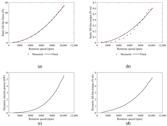
Figure 3. Bench test results for lift fans. (a) Lift fan static force test results and fitting curve; the estimated results are C_t = 4.2278. (b) Lift fan static torque test results and fitting curve; the estimated results are C_q = 0.2303. (c) Recorded dynamic electric power change with rotation speed. (d) Calculated results of the dynamic lift-fan torque.

As part of the dynamic modeling of the lift fan system, the derivative of the fan’s rotation speed can be represented by the following model:

$${\dot{\omega }}_f(t)=\frac{\min \left(\max \left(K_f\left({\omega }_{fc}\left(t-{\tau }_d\right)-{\omega }_f\left(t\right)\right)I_{rf},-Q_f\right),Q_{fp}+Q_f\right)}{I_{rf}}$$

(3)

where $K_f$ is the control bandwidth of the electronic speed controller (ECS, $K_f=30\mathrm{rad}/\mathrm{s}$), ${\tau }_d$ is the command delay for the rotation speed (${\tau }_d=10\mathrm{ms}$), and the rate of rotation speed is limited by $Q_{fp}$ and $Q_f$. Finally, the moment of the lift fan, $M_f$, is expressed in the body axis as follows:

$${\mathit{M}}_{\mathit{f}}=I_{rf}{\mathit{\omega }}_{\mathit{f}}\times \mathit{\Omega }+{\mathit{Q}}_{\mathit{f}}+\left(\mathit{C}\mathit{F}-\mathit{C}\mathit{G}+\mathit{B}\mathit{I}\mathit{A}\mathit{S}\right)\times {\mathit{T}}_{\mathit{f}}$$

(4)

In Equation (4), we have the following:

$$\begin{array}{l}{\mathit{\omega }}_{\mathit{f}}={\left[\begin{array}{ccc}0& 0& {\omega }_f\end{array}\right]}^T\\ \mathit{\Omega }={\left[\begin{array}{ccc}p& q& r\end{array}\right]}^T\\ {\mathit{T}}_{\mathit{f}}={\left[0\hspace{1em}0\hspace{1em}-T_f\right]}^T\\ {\mathit{Q}}_{\mathit{f}}={\left[0\hspace{1em}0\hspace{1em}{I}_{rf}{\dot{\omega }}_f+Q_f\right]}^T\\ \mathit{B}\mathit{I}\mathit{A}\mathit{S}=bias{\left[\cos {\mathsf{\Phi }}_f\hspace{1em}\sin {\mathsf{\Phi }}_f\hspace{1em}0\right]}^T\end{array}$$

(5)

where $bias$ is the eccentric size of the lift fan ($bias=0.005\mathrm{m}$); CF and CG are the positions of the lift fan and the center of gravity on the body axis, respectively; ${\mathsf{\Phi }}_f$ is the rotation angle of the fan, ranging from 0 to 2π radians; and p, q, and r are the UAV’s angular velocity.

2.3. Thrust Vector Model

Table 3 displays the second-order dynamic system model used to represent the thrust response to throttle input, accounting for position and rate limitations. It should be noted that positive rotation of the 3BSD nozzle generates negative moments and that the nozzle is aligned with the x-axis of the body frame.

Table 3. Effector characteristics of the UAV.

Effector	Explanation	Damping Ratio	Natural Frequency	Position Limit	Rate Limit
δe	Elevator angle	0.8	30 rad/s	[−30°, +30°]	±110 °/s
δa	Aileron angle	0.8	30 rad/s	[−30°, +30]	±110 °/s
δLSSD	Left SSD deflection angle	0.8	30 rad/s	[0°, 60°]	±110 °/s
δRSSD	Right SSD deflection angle	0.8	30 rad/s	[0°, 60°]	±110 °/s
δvq	3BSD nozzle pitch angle	1	10 rad/s	[0°, 90°]	±30 °/s
δvr	3BSD nozzle yaw angle	1	10 rad/s	[−15°, +15°]	±30 °/s
δvT	Turbojet engine throttle	1	1 rad/s	[0, 1]	0.3

The thrust vector changes with the rotation of the nozzle. To avoid a singularity at 90 degrees of pitch, the nozzle is first rotated around its pitch axis by an angle, δ_vr, and then the new frame is rotated around its yaw axis by an angle, δ_vq. The rotation matrix from the nozzle frame to the body frame is M_bT.

To prevent a singularity from occurring at 90 degrees of pitch, the thrust vector is adjusted through the rotation of the nozzle. Specifically, the nozzle is initially rotated around its pitch axis by an angle of δ_vq. Following this, the new frame is then rotated around its yaw axis by an angle of δ_vr to arrive at the desired orientation. The corresponding rotation matrix from the nozzle frame to the body frame is denoted as M_bT, and it can be expressed as follows:

$$M_{bT}=\left[\begin{array}{ccc}\cos {\delta }_{vr}& -\sin {\delta }_{vr}& 0\\ \sin {\delta }_{vr}& \cos {\delta }_{vr}& 0\\ 0& 0& 1\end{array}\right]\left[\begin{array}{ccc}\cos {\delta }_{vq}& 0& \sin {\delta }_{vq}\\ 0& 1& 0\\ -\sin {\delta }_{vq}& 0& \cos {\delta }_{vq}\end{array}\right]$$

(6)

The resulting expression for the thrust vector in the body frame is as follows:

$$\left[\begin{array}{c}{T}_{vx}\\ T_{vy}\\ T_{vz}\end{array}\right]=M_{bT}\left[\begin{array}{c}-{\delta }_{vT}{T}_{v\max }\\ 0\\ 0\end{array}\right]=\left[\begin{array}{c}{\delta }_{vT}{T}_{v\max }\cos {\delta }_{vq}\cos {\delta }_{vr}\\ {\delta }_{vT}{T}_{v\max }\cos {\delta }_{vq}\sin {\delta }_{vr}\\ -{\delta }_{vT}{T}_{v\max }\sin {\delta }_{vq}\end{array}\right]$$

(7)

To analyze the moments generated by the thrust vector, it is necessary to take the cross product of the thrust vector and its corresponding lever arm. This yields the following equation, which represents the moments generated by the thrust vector:

$$\left[\begin{array}{c}{M}_{vx}\\ M_{vy}\\ M_{vz}\end{array}\right]=\left[\begin{array}{ccc}0& 0& 0\\ 0& 0& -R_v\\ 0& R_v& 0\end{array}\right]\left[\begin{array}{c}{T}_{vx}\\ T_{vy}\\ T_{vz}\end{array}\right]=\left[\begin{array}{c}0\\ -R_v{\delta }_{vT}{T}_{v\max }\sin {\delta }_{vq}\\ R_v{\delta }_{vT}{T}_{v\max }\cos {\delta }_{vq}\sin {\delta }_{vr}\end{array}\right]$$

(8)

where R_v represents the distance from the nozzle to the center of gravity along the body’s x-axis, as shown in Figure 4. To balance the pitch moment generated by the thrust vector, the force that the lift fans should provide is calculated as follows:

$$T_f=\frac{R_v{\delta }_{vT}{T}_{v\max }\sin {\delta }_{vq}}{n{R}_f}$$

(9)

where n is the number of lift fans (n = 2), and R_f is the distance between the lift fan center and CG along the body x-axis. Equation (9), which represents the force required to balance the pitch moment, is used to determine the baseline rotation speed for pitch attitude control, as shown in the following equation:

$${\omega }_f=\sqrt{\frac{R_v{\delta }_{vT}{T}_{v\max }\sin {\delta }_{vq}}{n{R}_f\rho C_t{D}_f^4}}$$

(10)

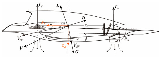
Figure 4. Longitudinal force analysis.

2.4. Aerodynamic Model

Computational fluid dynamics (CFD) methods are used to determine the UAV’s aerodynamic properties. However, for the sake of computational efficiency, the effects of the lift fans and thrust vector are not considered. Figure 5 displays the pressure contour of the aircraft, and three different grids are employed to check the mesh sensitivity of the CFD calculation: a fine mesh with $3{.1\times 10}^6$ nodes, a medium mesh with $2{.2\times 10}^6$ nodes, and a coarse mesh with ${8\times 10}^5$ nodes. In Figure 6a, the lift coefficient, C_L, increases with an increase in the angle of attack, but it does not reach the stall region within 12 degrees. The drag coefficient, C_D, on the other hand, rises monotonically as the angle of attack increases, as depicted in Figure 6b. It is worth noting that the drag coefficient obtained using the medium mesh is quite close to that obtained by the fine mesh. Therefore, unless otherwise stated in subsequent discussions, most of the results reported below are obtained on the medium mesh.

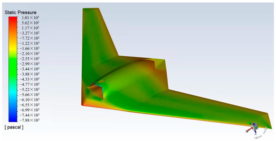
Figure 5. Pressure contour of the aircraft.

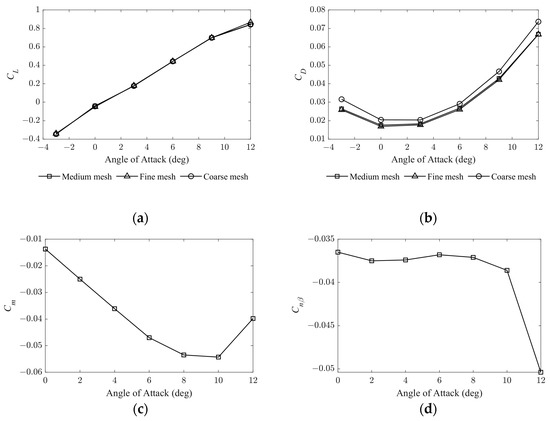
Figure 6. Longitudinal aerodynamic coefficients: (a) lift coefficient (sideslip angle β = 0), (b) drag coefficient (sideslip angle β = 0), (c) pitch-moment coefficient, and (d) directional static stability derivative (per radian).

The pitch moment coefficient, C_m, in Figure 6c indicates that the UAV gains longitudinal static stability before 10 degrees, so the maximum angle of attack for safe flight is set to 10 degrees. However, the UAV exhibits yaw static instability with a negative static directional-stability derivative $C_{n\beta }<0$ [27], which makes yaw control more challenging. This is shown in Figure 6d.

The SSD is used to control the yaw motion of the UAV. However, the control derivative, $C_{{n\delta }_{SDD}}$, exhibits nonlinear behavior at deflection angles below 10 degrees due to interactions between the SSD and the wing’s boundary layer [28], as shown in Figure 7. This nonlinearity makes yaw control more challenging. To address this, a bias angle [29] of 10 degrees is chosen for the SSD during yaw control.

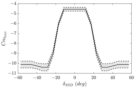
Figure 7. SSD yaw control moment derivative (per radian); the gray area is the continuous error bar for various angles of attack (angles of attack α = −6~12 deg).

Equations of motion with six degrees of freedom are developed for the UAV based on the previous analysis. These equations are then used for the performance analysis, control system design, and simulation of short landings. Table 3 summarizes the simulation inputs, and the outputs are the UAV’s states during simulation, including position, attitude angles, and angular rates.

3. Short-Landing Performance Analysis

3.1. Trim for Short Landing

To land the UAV safely, the sink rate, angle of attack, and velocity must be maintained for a steady approach. However, determining the baseline values for these parameters is challenging. To address this, the target UAV is trimmed at various angles of attack, sink rates, and velocities at a height of 50 m under control input restrictions. The trim speed ranges from 17 to 50 m/s, the angle of attack from 3 to 12 degrees, and the target sink rate from 0 to −4 m/s. The lift fan control is split into two parts: balancing the moment from ${\delta }_{vq}$ and compensating for ${\delta }_e$, as shown in Figure 8.

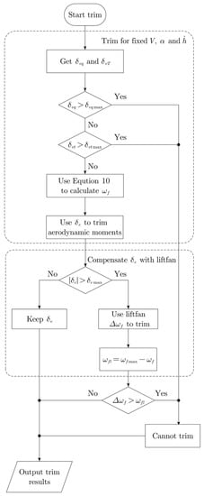
Figure 8. Trim procedure for short-landing performance analysis.

The results in Figure 9 show that the reachable area decreases as the angle of attack increases, and the velocity boundaries move to the left. As the angle of attack increases, the speed boundary decreases, allowing for a lower flight speed for the approach. However, a lower speed comes with a reduced maneuvering area, which increases the risk of the approach phase. Therefore, a balance must be made between the landing speed and flight safety, and the proper angle of attack and flight velocity must be selected during the short landing.

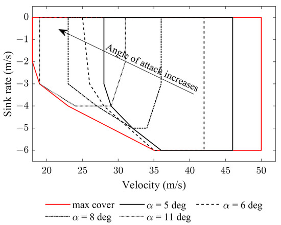
Figure 9. Reachable area for different angles of attack (angle of attack, α = 3~12 deg).

3.2. Attainable Linear and Pitch Angular Acceleration

To ensure flight safety during short landings, it is important to select an appropriate angle of attack and velocity for the aircraft. The conventional flying quality requirements based on maximum angular acceleration and attitude change in 1 s under an abrupt (0.3-s) ramp-control input [30] are not suitable for the flying-wing UAV, due to its unique size and inertial properties. Instead, a methodology can be used to identify the safest angle of attack for a given velocity by evaluating the maximum linear and angular acceleration generated by control effectors. This methodology involves selecting a series of equilibrium points [31] for the aircraft during a short landing. The longitudinal dynamic model of the UAV can be derived from Figure 4.

$$\begin{array}{l}{\dot{V}}_{gx}=-\frac{1}{m}\left(D\cos \gamma +L\sin \gamma -T\cos \left({\delta }_{vq}+\theta \right)+T_v\frac{R_v}{R_f}\sin {\delta }_{vq}\sin \theta \right)\\ {\dot{V}}_{gz}=-\frac{1}{m}\left(-D\sin \gamma +L\cos \gamma +T\sin \left({\delta }_{vq}+\theta \right)-gm+T_v\frac{R_v}{R_f}\sin {\delta }_{vq}\cos \theta \right)\end{array}$$

(11)

Equation (11) describes the longitudinal dynamic model of the UAV during a short landing, where $V_{gx}$ and $V_{gz}$ are the velocity components in the earth coordinate frame; L and D are the lift and drag forces in the wind coordinate frame; γ and θ are the flight path angle and pitch attitude angle, respectively; and g is the gravitational acceleration. To simplify the analysis, Equation (11) is expanded using a Taylor series, resulting in Equation (12), which considers only the first-order term of the expansion:

$$\dot{x}\approx {\dot{x}}_0+\underset{F\left(\cdot \right)}{\underbrace{{\left.\frac{\partial f\left(x,u\right)}{\partial x}\right|}_{\begin{array}{l}x=x_0\\ u=u_0\end{array}}}}\left(x-x_0\right)+\underset{G\left(\cdot \right)}{\underbrace{{\left.\frac{\partial f\left(x,u\right)}{\partial u}\right|}_{\begin{array}{l}x=x_0\\ u=u_0\end{array}}}}\left(u-u_0\right)$$

(12)

where the state vector is x = [$V_{gx}$ $V_{gz}$]^T, and the control input vector is u = [${\delta }_{vq}$ $T_v$]^T; x₀ and u₀ are the trimmed values for state and control; and F(·)∈R^2×2 and G(·)∈R^2×2 are vectors of nonlinear algebraic equations. The control input matrix, G(·), represents the acceleration response to the control inputs, as shown in the following equation:

$$G\left(\cdot \right)=\left[\begin{array}{cc}\frac{\partial {\dot{V}}_{gx}}{\partial {\delta }_{vq}}& \frac{\partial {\dot{V}}_{gx}}{\partial T_v}\\ \frac{\partial {\dot{V}}_{gz}}{\partial {\delta }_{vq}}& \frac{\partial {\dot{V}}_{gz}}{\partial T_v}\end{array}\right]$$

(13)

Equation (13) can be expanded using partial derivatives, as demonstrated in Equation (14).

$$\begin{array}{cc}\frac{\partial {\dot{V}}_{gx}}{\partial {\delta }_{vq}}=-\frac{T_v}{m}\left(\sin \left({\delta }_{vq}+\theta \right)+\frac{R_v}{R_f}\cos {\delta }_{vq}\sin \theta \right)& \frac{\partial {\dot{V}}_{gx}}{\partial T_v}=\frac{1}{m}\left(\cos \left({\delta }_{vq}+\theta \right)-\frac{R_v}{R_f}\sin {\delta }_{vq}\sin \theta \right)\\ \frac{\partial {\dot{V}}_{gz}}{\partial {\delta }_{vq}}=-\frac{T_v}{m}\left(\cos \left({\delta }_{vq}+\theta \right)+\frac{R_v}{R_f}\cos {\delta }_{vq}\cos \theta \right)& \frac{\partial {\dot{V}}_{gz}}{\partial T_v}=-\frac{1}{m}\left(\sin \left({\delta }_{vq}+\theta \right)+\frac{R_v}{R_f}\sin {\delta }_{vq}\cos \theta \right)\end{array}$$

(14)

Figure 10 displays the matrix G(·) calculated at a trimmed angle of attack of 4 degrees and various velocities. The gray area indicates a continuous error bar for the changing sink rate. In Figure 10a, tangential acceleration shows a negative correlation with the nozzle pitch angle, indicating that the UAV gains more deceleration capability as velocity decreases due to the larger trimmed nozzle pitch angle. In contrast, the throttle shows a positive correlation with tangential acceleration, which gradually weakens as the velocity decreases in Figure 10b. The nozzle pitch angle and throttle both exhibit a negative correlation with the normal acceleration in Figure 10c,d. The sink rate significantly affects the control efficiency for normal acceleration when using the nozzle pitch angle. The throttle shows better control for normal acceleration than the nozzle pitch angle. Overall, for better control effectiveness, it is preferable to use the throttle to control V_gz and the nozzle pitch angle to control V_gx, despite the control coupling phenomenon between the two.

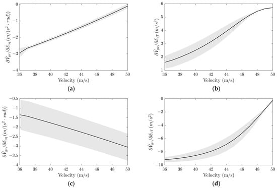
Figure 10. Control input matrix for acceleration (angle of attack α = 4 deg); the gray area is the continuous error bar for various sink rates (0~−4m/s): (a) G₁₁, (b) G₁₂, (c) G₂₁, and (d) G₂₂.

Equation (13) allows the acceleration control matrix to be calculated from trimmed results at different velocities and angles of attack. The attainable acceleration set (AAS) area can be evaluated from this matrix. The AAS area decreases with increasing trimmed velocity and increases with decreasing absolute sink rate, as shown in Figure 11a. In Figure 11b, the AAS area and attainable pitch angular acceleration (APAA) are compared, and they move in opposite directions as velocity increases. The equilibrium point, where the normalized AAS and APAA curves intersect, is shown in Figure 11c for different sink rates. The equilibrium points are calculated at various angles of attack and sink rates in Figure 11d, Figure 12a shows the AAS area [32] for a single trimmed point, with the throttle ranging from −10% to 10% and nozzle pitch angle from −10 to 10 degrees at an angle of attack of 6 degrees, and their mean velocity is presented in Figure 12b with an error bar. The equilibrium curve between the velocity and angle of attack provides the appropriate control command value for flight safety. Therefore, landing at the angle of attack and speed in Figure 12b maximizes the maneuvering margin during landing.

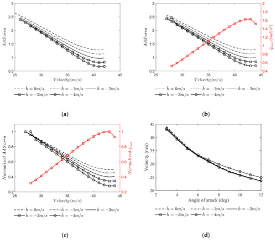
Figure 11. AAS and AMS calculation for short landing (angle of attack = 6 deg): (a) AAS area results, (b) AAS area and AMS results, (c) normalized AAS area and AMS results, and (d) equilibrium points for different sink rates.

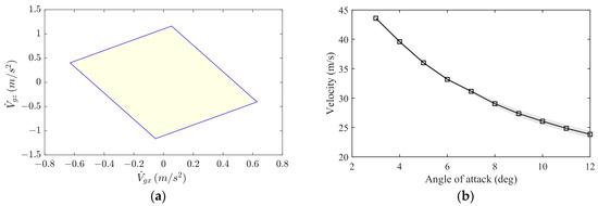
Figure 12. AAS area and equilibrium points curve: (a) AAS area (angle of attack = 6 deg, sink rate = −1 m/s, and velocity = 35 m/s) and (b) equilibrium points curve.

For flight safety during short landings, Figure 12b indicates an entering speed of 45 m/s in level flight condition with the nozzle pitch angle down approximately 45 degrees, as illustrated in Figure 13a. The lift fan should be set at 20%, as shown in Figure 13b. For continuous approaches, the recommended command values are a velocity of 35 m/s and angle of attack of 6 degrees, accounting for aerodynamic control effectiveness requirements for disturbance rejection.

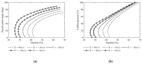
Figure 13. Trim results for short landing (angle of attack = 3 deg): (a) throttle and nozzle angle trim results and (b) throttle and lift fan trim results.

4. Flight Control System Design

4.1. Angular Rate and Attitude Controller

In an inner angular rate controller loop, the relationship between the control input and the dynamics of the UAV is obtained by the following equation:

$$\dot{\Omega }=\underset{f_{\left(\cdot \right)}}{\underbrace{I^{-1}{M}_{\left(\cdot \right)}-I^{-1}\left\{\Omega \times I\Omega \right\}}}+v_{\left(\cdot \right)}$$

(15)

where Ω = [p, q, r]^T represents the roll, pitch, and yaw angular rates in the body frame, respectively; v_(·) = [v_p, v_q, v_r]^T is the control acceleration input; I is the moment of the inertial matrix; and f_(∙) is the total disturbance added to the flying-wing UAV for each axis, which is composed of modeled coupling dynamics and unmodeled dynamics, M_(·). The unmodeled dynamics include external environmental disturbance and internal coupling dynamics. Then the Equation (15) can be reformulated as follows:

$$\left\{\begin{array}{l}\dot{x}=f_{\left(\cdot \right)}+v_{\left(\cdot \right)}\hfill \\ {\dot{f}}_{\left(\cdot \right)}=w\left(t\right)\hfill \end{array}\right.$$

(16)

To control the angular acceleration around the UAV’s body axis, an ESO-based control law is designed, where w(t) is the derivative of f_(∙) that is unknown but bounded. An ESO is capable of estimating the lumped disturbance caused by external disturbances, unmodeled dynamics, parameter variations, and complex nonlinear dynamics [33]. Dynamic compensation is then used based on the estimated results to linearize the model. For roll, pitch, and yaw control, a second-order linear ESO is designed, and the observer is expressed as follows:

$$\left\{\begin{array}{l}{\dot{z}}_1={\beta }_{01}\left(y-z_1\right)+z_2+v_{\left(\cdot \right)}\hfill \\ {\dot{z}}_2={\beta }_{02}\left(y-z_1\right)\hfill \end{array}\right.$$

(17)

In each angular rate control loop, y represents the angular rate measurements, while z₁ and z₂ are the estimated angular rates and disturbance. The observer gains, β₀₁ and β₀₂, can be determined using bandwidth methods [34].

$${\beta }_{01}=2{\omega }_{o,\left(\cdot \right)},{\beta }_{02}={\omega }_{o,\left(\cdot \right)}{}^2$$

(18)

The ESO’s observation bandwidth for each angular rate control loop is denoted as ${\omega }_{o,\left(\cdot \right)}$. The error dynamics of the ESO can be calculated as follows:

$$\left\{\begin{array}{l}{\dot{e}}_1=-{\beta }_{01}{e}_1+e_2\hfill \\ {\dot{e}}_2=-{\beta }_{02}{e}_1-w\left(t\right)\hfill \end{array}\right.$$

(19)

where $e_1{=z}_1 -x$ and $e_2{=z}_2 {-f}_{\left(·\right)}$ are the estimated error. The characteristic polynomial of Equation (19) can be expressed as follows:

$$\lambda \left(s\right)=s^2+{\beta }_{01}s+{\beta }_{02}$$

(20)

With positive observer gains, the roots of the characteristic polynomial in Equation (20) are all in the left half plane, ensuring the ESO’s bounded-input–bounded-output (BIBO) stability [35]. A proportional controller is designed, and the estimated disturbance is given as follows:

$$v_{\left(\cdot \right)}=k_{\left(\cdot \right)}\left({\Omega }_c-\Omega \right)-z_{2\left(\cdot \right)}$$

(21)

The proportional controller is designed to control the estimated disturbance in each control channel. The proportional gains or control bandwidth of the closed loop are denoted by $k_{\left(·\right)}\in {(k}_p{,k}_q{,k}_r)$. The estimated disturbance for each control channel is denoted by $z_{2\left(\cdot \right)}$, and ${\Omega }_c={\left[p_c{,q}_c{,r}_c\right]}^{\mathrm{T}}$ is the command angular rate. The stability analysis of the ESO-based controller and the relationship between the error bounds and ADRC bandwidth are presented in Reference [34]. The rate of change in attitude angles can be expressed as follows:

$$\left[\begin{array}{c}\dot{\varphi }\\ \dot{\theta }\\ \dot{\psi }\end{array}\right]=\left[\begin{array}{ccc}1& \sin \varphi \tan \theta & \cos \varphi \tan \theta \\ 0& \cos \varphi & -\sin \varphi \\ 0& \sin \varphi /\cos \theta & \cos \varphi /\cos \theta \end{array}\right]\left[\begin{array}{c}p\\ q\\ r\end{array}\right]$$

(22)

where ϕ, θ, and ψ are roll, pitch, and yaw angles, respectively. The desired rotational rates can be achieved using Equation (22), which gives the following [36]:

$$\left[\begin{array}{c}{p}_c\\ q_c\end{array}\right]={\left[\begin{array}{cc}1& \sin \varphi \tan \theta \\ 0& \cos \varphi \end{array}\right]}^{-1}\left\{\left[\begin{array}{c}{v}_{\varphi }\\ v_{\theta }\end{array}\right]-\left[\begin{array}{c}\tan \theta /\cos \varphi \\ -\tan \varphi \end{array}\right]r\right\}$$

(23)

where v_ϕ and v_θ are the desired dynamic responses for roll and pitch attitude, which are calculated using the following equation:

$$\left[\begin{array}{c}{v}_f\\ v_{\theta }\end{array}\right]=\left[\begin{array}{cc}{k}_f& 0\\ 0& k_{\theta }\end{array}\right]\left[\begin{array}{c}{f}_c-f\\ {\theta }_c-\theta \end{array}\right]\left[\begin{array}{c}{p}_c\\ q_c\end{array}\right]$$

(24)

The slow outer attitude control loop [37] is governed by an NDI-based control law, which is a model-based strategy for controlling nonlinear dynamic systems. The input-output linearization method, based on NDI control theory [38], is utilized due to the precise measurement of the aircraft’s kinematic parameters, using an inertial navigation system (INS). This enables the design of a simple linear controller for the resulting system, where the command attitude angles [ϕ_c, θ_c] and proportional control gains [k_ϕ, k_θ] are utilized. To achieve coordinated flight, it is necessary to regulate the sideslip angle, β, instead of the yaw angle ψ, particularly for tailless aircraft. The desired yaw angular rate can be obtained by using the following equation, as proposed in Reference [39]:

$$r_c=-k_{\beta }\left({\beta }_c-\beta \right)+\frac{g\sin \varphi \cos \theta }{V}$$

(25)

where β_c is the command sideslip angle, which is set to zero throughout the short-landing process, and k_β is the control gain. The complete diagram for the attitude and angular rate control loop is illustrated in Figure 14.

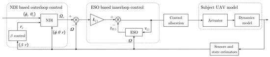
Figure 14. Complete control diagram for inner and outer loop control.

4.2. Control Allocation

In the UAV configuration depicted in Figure 1, both the roll and yaw control are achieved by the aileron and SSD. The control allocation process in this configuration can utilize a pseudo-inverse method, which is outlined below:

$$\left[\begin{array}{c}{\delta }_{ac}\\ {\delta }_{SDDc}\end{array}\right]={\left[\begin{array}{cc}{L}_{{\delta }_a}& 0\\ 0& N_{{\delta }_{SDD}}\end{array}\right]}^{-1}\left[\begin{array}{c}{v}_p\\ v_r\end{array}\right]$$

(26)

where δ_ac and δ_SDDc are the aileron and SSD command values, and the roll and yaw control effectiveness parameters are as follows:

$$\begin{array}{l}{L}_{{\delta }_a}=\frac{1/2\rho V^{2}Sb{C}_{l{\delta }_a}}{I_{xx}}\\ N_{{\delta }_{SDD}}=\frac{1/2\rho V^{2}Sb{C}_{n{\delta }_{SDD}}}{I_{zz}}\end{array}$$

(27)

where C_lδa is the control derivative of the aileron. The control allocation, Equation (26), does not consider the coupling effect between the SDD and aileron, as it is treated as a disturbance that can be estimated by the ESO. The control allocation for the pitch channel involves both aero surfaces and lift fans, which differ from the roll and yaw channels. Due to the distinct response characteristics of the elevator and lift fans, both a high-frequency and low-frequency control allocation for the pitch channel are carried out, as illustrated in Figure 15.

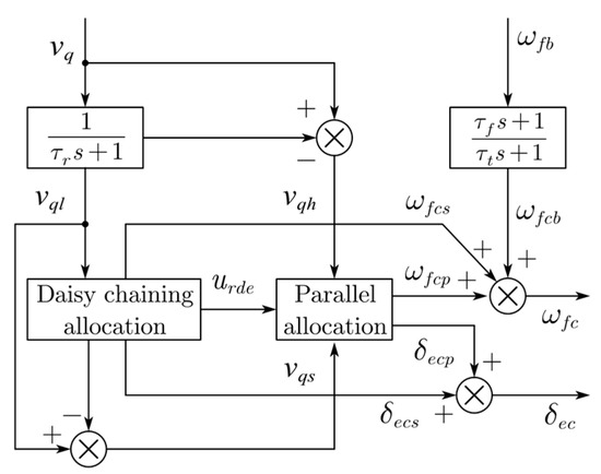
Figure 15. Pitch channel control allocation.

To allocate the control inputs for the pitch channel, the desired pitch angular acceleration, v_q, is first filtered using a first-order lag transfer function with a time constant of 1 s (${\tau }_r=1\mathrm{s}$). The resulting desired pitch control value is then split into two components: a low-frequency part (LFP), v_ql; and a high-frequency part (HFP), v_qh. The LFP is allocated using a daisy-chaining method [32], which involves calculating the elevator command value as follows:

$${\delta }_{ecs}=\max \left(\min \left(v_{ql}/M_{{\delta }_e},{\delta }_{e\max }\right),{\delta }_{e\min }\right)$$

(28)

where $M_{{\delta }_e}$ is the control effectiveness parameter of the elevator and can be calculated as follows:

$$M_{{\delta }_e}=\frac{1/2\rho V^{2}Sc{C}_{m{\delta }_e}}{I_{yy}}$$

(29)

where $C_{{m\delta }_e}$ is the control derivative of the elevator. If the elevator deflection angle reaches its limits, the lift fan is utilized to compensate for the LFP. The left LFP, u_qs, is then obtained through the lift fan:

$$\begin{array}{l}{v}_{qs}=v_{ql}-M_{{\delta }_e}{\delta }_{ecs}\\ {\omega }_{fcs}=v_{qs}/M_{fan}\end{array}$$

(30)

where ω_fcs is the command value of the lift fan, and M_fan is the control effectiveness parameter of the lift fan, as follows:

$$M_{fan}=\frac{2n\rho C_t{\omega }_f{D}_f^4{R}_f}{I_{yy}}$$

(31)

Secondly, the HFP is allocated via parallel allocation. The elevator’s and lift fan’s residual control powers are denoted as u_rde and u_rfan, respectively. When v_qh ≥ 0, the output of the parallel output is given by the following:

$$\left\{\begin{array}{l}k=v_{qh}/\left(u_{rde}+u_{rfan}\right)\hfill \\ \begin{array}{l}{\omega }_{fcp}=k\left({\omega }_{f\max }-{\omega }_{fcs}\right)\\ {\delta }_{ecp}=k\left({\delta }_{e\max }-{\delta }_{ecs}\right)\end{array}\hfill \end{array}\right.$$

(32)

otherwise, we have the following:

$$\left\{\begin{array}{l}k=v_{qh}/\left(u_{rde}+u_{rfan}\right)\hfill \\ \begin{array}{l}{\omega }_{fcp}=k\left({\omega }_{f\min }-{\omega }_{fcs}\right)\\ {\delta }_{ecp}=k\left({\delta }_{e\min }-{\delta }_{ecs}\right)\end{array}\hfill \end{array}\right.$$

(33)

where we have the following:

$$\begin{array}{l}{u}_{rde}=\left\{\begin{array}{c}{M}_{{\delta }_e}\left({\delta }_{e\max }-{\delta }_{ecs}\right),v_{qh}<0\\ M_{{\delta }_e}\left({\delta }_{e\min }-{\delta }_{ecs}\right),v_{qh}\ge 0\end{array}\right.\\ u_{rfan}=\left\{\begin{array}{c}{M}_{fan}\left({\omega }_{f\max }-{\omega }_{fcs}\right),v_{qh}\ge 0\\ M_{fan}\left({\omega }_{f\min }-{\omega }_{fcs}\right),v_{qh}<0\end{array}\right.\end{array}$$

(34)

In Equation (34), ${\omega }_{f\max }$ and ${\omega }_{f\min }$ represent the maximum and minimum rotation speeds of the lift fans, respectively. These values are selected to be between −80% and 80% of the baseline rotation speed command, which is calculated using the throttle command value in Equation (10). To synchronize the responses of the turbojet engine and lift fans, a first-order lead-lag controller is applied with time constants of 0.1 s (${\tau }_f=0.1\mathrm{s}$) and 1 s (${\tau }_t=1\mathrm{s}$) for the engine and lift fans, respectively. The baseline rotation speed command passes through the lead-lag control unit and is denoted as ${\omega }_{fcb}$ in Figure 15. The output of the pitch control allocation is a combination of the baseline part, the daisy chaining allocation part, and the parallel allocation part, as expressed by the following equation:

$$\left\{\begin{array}{l}{\omega }_{fc}={\omega }_{fcb}+{\omega }_{fcs}+{\omega }_{fcp}\hfill \\ {\delta }_{ec}={\delta }_{ecs}+{\delta }_{ecp}\hfill \end{array}\right.$$

(35)

4.3. Angle of Attack Control

For flying wing aircraft, changes in the angle of attack significantly affect longitudinal static stability. Poor longitudinal and lateral static stability can pose a serious threat to flight safety. Therefore, the angle of attack, denoted by α, is chosen as the control object for the outer loop, which generates a pitch angular rate command for the inner control loop. Neglecting the lateral and directional coupling dynamics, the linearized model for the angle of attack can be expressed as follows [17]:

$$\dot{\alpha }=-Z_{\alpha }\alpha +q+Z_{{\delta }_e}{\delta }_e$$

(36)

where we have the following:

$$\begin{array}{l}{Z}_{\alpha }=\frac{1/2\rho V^{2}S{C}_{L\alpha }}{mV}\\ Z_{{\delta }_e}=\frac{1/2\rho V^{2}S{C}_{L{\delta }_e}}{mV}\end{array}$$

(37)

where $C_{L\alpha }$ is the lift curve slope, and $C_{{L\delta }_e}$ is the derivative of the lift coefficient to the elevator. The value of $C_{{L\delta }_e}$ is insignificant when compared to $C_{L\alpha }$, resulting in the simplification of the transfer function for the pitch angular rate to angle of attack:

$$\frac{\alpha \left(s\right)}{q\left(s\right)}=\frac{1}{s+Z_{\alpha }}$$

(38)

Consider the closed-loop dynamics of the pitch angular rate in the system. If it is assumed to be a first-order low-pass filter, then the transfer function for the angle of attack command to the measured output can be simplified as a second-order nominal model with the angle of attack controller. This can be expressed as follows:

$$\frac{\alpha \left(s\right)}{{\alpha }_c\left(s\right)}=\frac{k_{\alpha }{k}_q}{s^2+k_{q}s+k_{\alpha }{k}_q}$$

(39)

The control diagram of the angle of attack is shown in Figure 16.

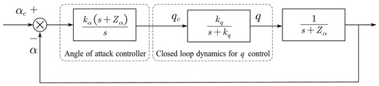
Figure 16. Diagram of the angle of attack controller.

The controller gain, k_α, can be calculated using the desired bandwidth and damping ratio of the closed-loop system. In this case, the damping ratio is selected to be 0.8, and then k_α can be calculated using the following formula:

$$k_{\alpha }=k_q/{1.6}^2$$

(40)

4.4. Sink Rate and Velocity Control

According to the analysis in Section 3, the 3BSD’s nozzle pitch angle is utilized to control the UAV’s velocity, and its sink rate is controlled by using the turbojet engine throttle. For velocity control, a simple proportional-integral (PI) controller is applied to obtain the desired tangential acceleration, as the following equation:

$$k_{vi}{\displaystyle {\int }_0^t\left(V_c-V\right)dt}-k_{vp}V={\dot{V}}_{des}$$

(41)

where we have the following:

$$\begin{array}{l}{k}_{vp}=2{\zeta }_T{\omega }_T\\ k_{vi}={\omega }_T^2\end{array}$$

(42)

where ω_T is the closed-loop bandwidth, and ${\mathsf{\zeta }}_T$ is the damping ratio which is set to 0.8 to reduce overshoot. The command value of the nozzle pitch angle is achieved using the following equation:

$${\delta }_{vqc}=\max \left(\min \left(\frac{-m\left({\dot{V}}_{des}-g\sin \gamma \right)}{{\delta }_{vTc}{T}_{v\max }\cos {\delta }_{vqb}}{\delta }_{vqb},{\delta }_{vq\max }-{\delta }_{vqb}\right),-{\delta }_{vqb}\right)$$

(43)

where ${\delta }_{vTc}$ is the throttle command value, ${\delta }_{vqb}$ is the baseline nozzle pitch angle given by the setting at the beginning of short landing, and ${\delta }_{vq\max }$ is the maximum nozzle pitch angle. The output command of the nozzle pitch angle is equal to the sum of ${\delta }_{vqc}$ and ${\delta }_{vqb}$.

For sink rate control, two controllers are used for different short-landing stages. The first uses the pitch angle to control the sink rate [22], and the controller is activated in the deceleration period. The closed-loop dynamics of the pitch angle are regarded as a first-order low-pass filter, as shown in Figure 17a. The closed-loop transfer function from γ_c to γ is as follows:

$$\frac{\gamma \left(s\right)}{{\gamma }_c\left(s\right)}=\frac{k_{\theta }{k}_{\gamma }{Z}_{\alpha }}{s^2+k_{\theta }s+k_{\theta }{k}_{\gamma }{Z}_{\alpha }}$$

(44)

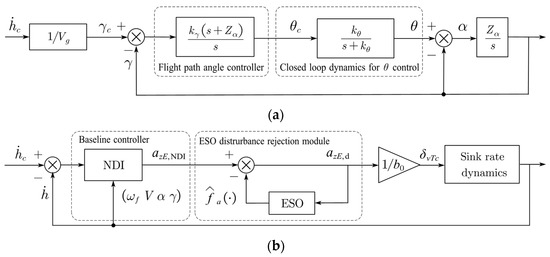
Figure 17. Sink rate control diagram: (a) control sink rate obtained using pitch attitude angle and (b) control sink rate obtained using the throttle.

To reduce overshoot, the damping ratio of the second-order system in Equation (44) is selected to be 0.8. The controller gain, k_γ, can then be calculated through pole placement:

$$k_{\gamma }=k_{\theta }/\left({1.6}^2{Z}_{\alpha }\right)$$

(45)

The other sink rate controller uses the throttle to control the sink rate and is activated during the approach stage, as depicted in Figure 17b.

For sink rate control in the approach stage, the vertical dynamics of the UAV are given by the following equation:

$$-{\dot{V}}_{gz}/\cos \gamma =Z_{\alpha }\alpha V\cos \alpha -g\cos \gamma +\frac{1/2\rho V^{2}S{C}_D\sin \alpha }{m}+\frac{{\delta }_{vT}{T}_{v\max }\sin {\delta }_{vq}}{m}+\frac{n\rho C_t{\omega }_f{}^2{D}_f^4}{m}$$

(46)

where we have the following:

$${\dot{V}}_{gz}=-\dot{h}$$

(47)

Equation (46) can be rewritten as follows:

$${\dot{V}}_{gz}=\underset{A_1}{\underbrace{-Z_{\alpha }\alpha V+g\cos \gamma -\frac{n\rho C_t{D}_f^4}{m}{\omega }_{fcb}{}^2}}\underset{b_0}{\underbrace{-\frac{T_{v\max }\sin {\delta }_{vq}}{m}}}{\delta }_{vTc}+f_a\left(\cdot \right)$$

(48)

where A₁ is the known part of the sink rate control, b₀ is the control effectiveness parameter for the throttle, and f_a(·) is the lumped disturbance, which includes the unmodeled dynamics and external disturbances. An NDI controller is designed as a baseline sink rate controller, as shown in Figure 17b. The output of the baseline controller is formulated as follows:

$$a_{zE,NDI}=-k_{sr}\left({\dot{h}}_c-\dot{h}\right)-A_1$$

(49)

where k_sr is the designed sink rate control bandwidth. Similar to the approach in Section 4.1, to improve the tracking performance, a second-order ESO is designed to estimate the disturbance, f_a(·), as follows:

$$\left\{\begin{array}{l}{\dot{z}}_{1,sr}={\beta }_{01,sr}\left(y-z_{1,sr}\right)+z_{2,sr}+a_{zE,d}\hfill \\ {\dot{z}}_{2,sr}={\beta }_{02,sr}\left(y-z_{1,sr}\right)\hfill \end{array}\right.$$

(50)

where z_1,sr and z_2,sr are the estimation results of the sink rate and disturbance, and β_01,sr and β_02,sr are the ESO’s observation gain, which can be determined as follows [35]:

$${\beta }_{01,sr}=2{\omega }_{o,sr},{\beta }_{02,sr}={\omega }_{o,sr}{}^2$$

(51)

where ω_o,sr is the ESO’s observation bandwidth. In Equation (50), a_zE,d is the desired vertical acceleration and can be expressed as follows:

$$a_{zE,d}=a_{zE,NDI}-z_{2,sr}$$

(52)

Finally, the output throttle command is as follows:

$${\delta }_{vTc}=\frac{a_{zE,d}}{b_0}$$

(53)

4.5. Overall Control Structure

The overall control structure of the flying wing UAV, which includes the inner rotational controller and outer translational controller, is depicted in Figure 18. The methods for cross-track error (CTE) control and vertical offset control are further discussed in Section 5.

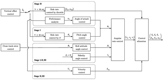
Figure 18. Overall control structure for short landing.

5. Short-Landing-Strategy Design

5.1. Short-Landing Procedures

The four-stage short-landing process of the flying wing UAV, shown in Figure 19, is designed based on the analyses presented earlier. The process commences at Point A, where the UAV is at a height of 50 m and a speed of around 64 m/s, with a non-zero sink rate. The stages of the process are as follows:

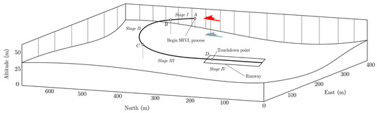
Figure 19. Short-landing process.

Stage I: The UAV reduces its nozzle pitch angle at a rate of 15 °/s, with the throttle fixed at the current value. The bank angle is adjusted to minimize the cross-track error by using the zero sideslip angle command, and the sink rate is controlled by the pitch attitude angle, as discussed in Section 4.4. The sink rate command is based on the distance to the target touchdown point, as explained in Section 5.2. When the nozzle pitch angle reaches 45 degrees, the short landing proceeds to the next stage.

Stage II: In this stage, the lateral and sink rate controls are the same as those in Stage I. The nozzle pitch angle is utilized to control the velocity, and the velocity command is set to 35 m/s to prevent the inefficiency of the elevator under low dynamic pressure. The short landing advances to Stage III when the velocity decreases to below 36 m/s or the deceleration process lasts more than 20 s.

Stage III: In this stage, the angle of attack is set to 6 degrees based on the analysis presented in Section 3, and the sink rate is regulated by the throttle, which is different from the scenarios in Stages I and II. The lateral control remains the same as in Stage II. Additionally, the maximum bank angle command is restricted to 5 degrees below 2 m above the ground to avoid wing strike. The UAV maintains its speed by nozzle pitch angle deflection until it touches down.

Stage IV: Upon touchdown, the longitudinal control mode switches to pitch angular rate control, and the command is set to zero. The objective of this stage is to slow down the UAV by turning off the engine and braking while keeping it on the runway via front-wheel steering.

5.2. Lateral and Vertical Guidance

The lateral control’s objective is to eliminate the CTE error by using the bank angle control. The bank angle command is calculated as follows:

$${\varphi }_c=\arctan \left({\dot{\psi }}_{des}{V}_g/g\right)$$

(54)

where we have the following:

$$\begin{array}{l}{\dot{\psi }}_{des}={\omega }_{as}\Delta \psi \\ \Delta \psi =\left[\left({\psi }_{des}-{\psi }_t+\pi \right)\mathrm{mod}2\pi \right]-\pi \\ {\psi }_{des}=\arcsin \left({\omega }_y\Delta Y/V_g\right)\end{array}$$

(55)

where ΔY is the CTE, V_g is the ground velocity, ${\psi }_t$ is the heading angle, and ω_y is the CTE control bandwidth. The course angle error, Δψ, is limited between −π and π and is fed to a controller with proportional gain, ω_as, whose output is the desired rate of change of course angle.

To improve the accuracy of the touchdown point, the sink rate command is adjusted online based on the distance from the landing point. The sink rate command is given by the following equation:

$${\dot{h}}_c=-\left[V_g\cos \left(\left|{\psi }_{rw}-{\psi }_t\right|\right)\right]\arctan \left(H/X_{des}\right)$$

(56)

In Figure 20, the projection of the line of sight (LOS) in the direction of the runway is denoted as X_des, the direction angle of the runway is ψ_rw, and H is the altitude above ground level (AGL). It is important to note that when X_des approaches zero, the sink rate command tends to infinity according to Equation (56). In order to ensure the landing gear’s strength, the sink rate command is limited to a range of −2 to 0 m/s, and when X_des is less than 5 m, the sink rate command remains constant.

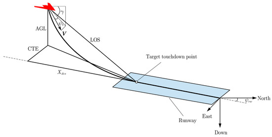
Figure 20. Sink rate and bank angle command calculation.

6. Simulation Verification and Discussion

6.1. Effectiveness of the Short-Landing Strategy

The proposed method’s effectiveness was evaluated through numerical simulations, which only considered events up to the touchdown, and the simulations stopped once the UAV’s landing gear was compressed. Table 4 provides a summary of the control parameters, while Figure 21 displays the three-dimensional (3D) trajectory of a short landing.

Table 4. Inner and outer loop control parameters.

Parameter	Explanation	Value	Parameter	Explanation	Value
kp	p control bandwidth	6	kθ	Pitch angle control gain	1.2
kq	q control bandwidth	10	kβ	Side slip angle control gain	0.8
kr	r control bandwidth	6	ksr	Sink rate control gain	0.4
ωo,p	p observation bandwidth	7	ωo,sr	Sink rate observation bandwidth	1
ωo,q	q observation bandwidth	5	ωT	Velocity control bandwidth	0.25
ωo,r	r observation bandwidth	10	ωy	CTE control bandwidth	0.15
kϕ	Roll angle control gain	1.2	ωas	Course angle control gain	0.5

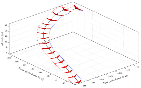
Figure 21. Three-dimensional trajectory of short landing.

The use of thrust vector control in the short-landing process allows for a reduction in touchdown speed, which, in turn, reduces the required length of the runway. Without the thrust vector and lift fans, the touchdown speed of the UAV can be calculated [27] by using the lift coefficient in Figure 6b, resulting in a speed of approximately 46 m/s. However, with the thrust vector control, the touchdown speed can be reduced to 35 m/s, which is 24% lower than the classic speed. This reduction in touchdown speed results in a corresponding 24% reduction in the length of the runway, as determined by the integral relationship between velocity and position. As a result, for a given runway, the short-landing technique allows for the recovery of more payload with the same landing speed as the classic landing process.

The simulation results are presented in Figure 22, which demonstrates the effectiveness of the ESO-based angular rate control loops during the short-landing process. Specifically, the three-axis decoupled control achieved a side slip angle under 1.2 degrees, resulting in a coordinated turn in Figure 22d,h. The sink rate during the switch to short-landing mode was approximately −1 m/s, as shown in Figure 22e. During Stage I, the nozzle pitch angle was increased to 45 degrees, and the throttle command was set to 0.45, as depicted in Figure 22l,n. As the nozzle angle decreased, the rotation speed increased to 8000 rpm to balance the moment produced by the vectored thrust. In Stage II, which began when the nozzle angle reached 45 degrees, the throttle was fixed, and the nozzle pitch angle was adjusted to reduce the speed. Figure 22l shows that the nozzle pitch angle was increased to 90 degrees in Stage II to reduce the speed from 60 m/s to 35 m/s. During both Stage I and Stage II, the pitch attitude angle controlled the sink rate, but the sink rate was still affected by changes in the bank angle, as shown in Figure 22g,e.

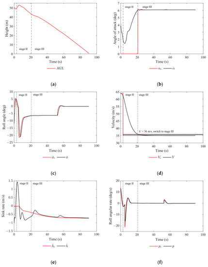
Figure 22. Nominal simulation results of short landing: (a) AGL (Above Ground Level)response, (b) angle-of-attack response, (c) velocity response, (d) roll-angle response, (e) sink-rate response, (f) roll-angular-rate response, (g) pitch-angle response, (h) side-slip-angle response, (i) pitch-angle-rate response, (j) Yaw-angle-rate response, (k) actuator response, (l) nozzle-pitch-angle response, (m) lift-fan-rotation-speed response, and (n) throttle response.

Next, the short-landing process entered Stage III, where the nozzle-pitch angle was used to maintain a constant velocity, the throttle was used to control the sink rate, and a combination of the elevator and the lift fan controlled the angle of attack. The baseline angle-of-attack command value was 6 degrees, and Figure 22b shows that there was no steady-state error in tracking. When the sink-rate control mode was switched to the ESO-based control in Stage III, the sink-rate controller performed well in terms of its tracking performance. At around 58 s, a disturbance in the roll angular rate occurred, but it quickly decayed, as shown in Figure 22e, ultimately improving the landing accuracy. The maximum deflection of the elevator was approximately −18 degrees, which corresponds to approximately 60% of its maximum value, as illustrated in Figure 22k.

6.2. Flight Boundary Protection with the Additional Angle-of-Attack Command

The findings from the short-landing performance study in Section 3 indicate that setting the angle-of-attack command at 6 degrees can achieve good results. However, when certain parameters are perturbed, such as lift coefficient, mass properties, and lift fan force, the sink rate may become uncontrollable. In the first scenario, if the lift coefficient is less than the estimated value or the UAV’s weight exceeds the pre-calculated value, the nominal reference angle of attack may not generate enough lift force to maintain the sink-rate command. This is demonstrated in Case 2 in Figure 23a, where the UAV cannot sustain its sink rate and falls to the ground before reaching the target point. In the second scenario, if the lift coefficient is greater than the CFD calculation results, the UAV moves up and down in response to the velocity command, as observed in Case 1. Both of these scenarios should be avoided to ensure short-landing precision and safety.

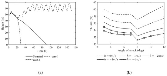
Figure 23. Simulation and analysis for the angle-of-attack control: (a) fixed angle-of-attack command simulation results, with Case 1 as −20% perturbation of the nominal lift coefficient and Case 2 as +20% perturbation of the nominal lift coefficient; and (b) trim results for different angles of attack and sink rates (at 80 percent of lift fan’s maximum rotation speed).

During short landing, the throttle is used to compensate for the aerodynamic lift force, while a portion of the lift fan’s control power is used to balance the pitch moment produced by the vectored thrust. In order to ensure that there is enough pitch controllable margin to meet the extra pitch control moment requirement, 20% of the lift fan’s control power is allocated to pitch angular rate control. The trim results, using 80% of the lift fan’s control power, are presented in Figure 23b.

To prevent the throttle command value from exceeding the lift fan’s trim boundary, an additional angle-of-attack command is calculated and added to the baseline value. This additional command can be expressed as follows:

$$\Delta {\alpha }_c\left(t\right)=\min \left(\max \left(\frac{\left({\delta }_{vTc}-{\delta }_{vTs}\right)T_{v\max }\sin {\delta }_{vq}}{Z_{\alpha }mV},-\Delta {\alpha }_c\left(t-\Delta T\right)\right),{\alpha }_{c\max }-{\alpha }_c\left(t\right)\right)$$

(57)

where ${\Delta \alpha }_c\left(t\right)$ and ${\Delta \alpha }_c\left(t-\Delta T\right)$ are the current and previous additional angle-of-attack command values, respectively; ${\alpha }_{c\max }$ is the maximum angle of attack command value, which is set at 10 degrees; and ${\delta }_{vTs}$ is the threshold of the throttle, which is set to 0.6 based on the trim results in Figure 23b. In Stage III, the current angle-of-attack value is used to determine the angle-of-attack command value, and the additional angle-of-attack command value is added to compensate for the perturbations in lift coefficient, mass properties, and lift fan force, ensuring precise and safe short landings:

$${\alpha }_c\left(t\right)=\alpha \left(t\right)+\Delta {\alpha }_c\left(t\right)$$

(58)

6.3. Sink-Rate Control under Wind Gust

To evaluate the performance of the ESO-based sink-rate control proposed in Section 4.4, the implicit NDI controller was chosen for comparison, using the same control bandwidth. Referring to Equation (41), the control law for sink rate control can be expressed as follows:

$$-a_{zE,d}=k_i{\displaystyle {\int }_0^t\left({\dot{h}}_c-\dot{h}\right)dt}-k_p\dot{h}+A_1$$

(59)

where k_p and k_i are the control parameters, which can be determined by referring to Equations (41) and (42). The wind-gust model is described as follows:

$$\left\{\begin{array}{cc}{u}_g=\frac{u_m}{2}\left(1-\cos \left(\frac{\pi x}{d_x}\right)\right)& 0\le x\le d_x\\ w_g=\frac{w_m}{2}\left(1-\cos \left(\frac{\pi x}{d_z}\right)\right)& 0\le x\le d_z\end{array}\right.$$

(60)

where u_g is the gust in the u-axis; w_g is the gust in the w-axis; x is the integration of velocity; d_x = 120 m and d_z = 80 m is the gust length; u_m = 3.5 m/s; and w_m = 3 m/s is the gust amplitude [40]. As shown in Figure 24, it can be observed that there is no significant difference in the sink-rate response when there is no wind. However, when the wind is introduced at 32 s, the ESO-based sink-rate controller exhibits a better disturbance rejection capability with rapid convergence, while the NDI controller continues to oscillate and shows a trend of divergence. Therefore, it can be concluded that the ESO-based sink-rate controller performs better when faced with external disturbances.

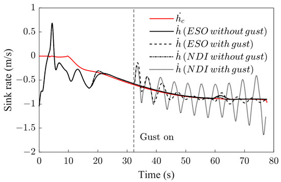
Figure 24. Sink rate control under the wind gust.

6.4. Robustness against Model Mismatch

The proposed short-landing technique must consider various uncertainties and modeling errors to ensure flight safety. Examples of these uncertainties include thrust-induced uncertainties [41], ground-effect uncertainties [25], uncertainties due to the interaction between lift fans and wings, inertial parameter uncertainties, and uncertainties in thrust loss induced by the increase in nozzle pitch angle [42]. To test the robustness of the proposed technique, an MC simulation was conducted with 500 simulations, where model parameters were perturbed in the nonlinear model, as shown in Table 5.

Table 5. Model parameters bias.

Parameter	Explanation	Bias Range
M	Mass	±1 kg
cgx, cgy, cgz	Centre of gravity	±5%
qbar	Dynamic pressure	±15%
CLα	Lift coefficient derivative	±20%
Clβ	Roll moment coefficient derivative	±20%
Clδa, Cmδe, Cnδr	Roll, pitch, and yaw control derivatives	±20%
T	Engine thrust	−20~0%
Tf	Lift fan force	−20~0%
Ixx, Iyy, Izz	Moment of inertia	±20%
Clp, Cmq	Damping moment coefficient derivatives	±50%
CD0	Drag coefficient	0~20%

During the MC simulation, it was observed that, although the angle-of-attack command value was set to 6 degrees, the steady-state angle-of-attack response was between 3 and 9 degrees. This shows that the flight boundary protection method proposed in Section 6.2 is effective in protecting the flight boundary. Figure 25a illustrates the steady-state angle-of-attack response for the 500 simulations conducted during the MC simulation.

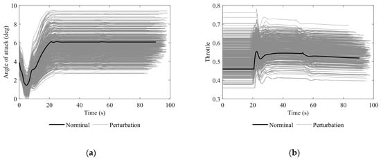
Figure 25. States response of the MC simulation: (a) angle-of-attack response and (b) throttle response.

To prevent the throttle command value from going beyond its trim boundary, an additional angle-of-attack command is generated by the flight boundary protection method when the throttle command value exceeds 0.6, as shown in Figure 25b.

To assess the effect of the additional angle-of-attack command on the success rate of short landings, 500 MC simulations were performed without flight envelope protection and using the perturbation range of parameters from Table 5. A landing was considered unsuccessful if the distance error between the touchdown point and the intended touchdown point exceeded 5 m, or if the aircraft failed to land. Among the 500 simulations, 127 short landings failed due to early touchdown or excessive pitch oscillations during the approach, as illustrated in Figure 23. The success rate of short landings was found to be 74.6%, and Figure 26 illustrates the angle-of-attack response of successful landings.

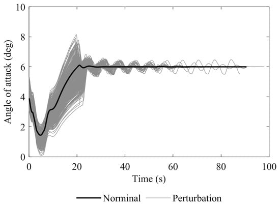
Figure 26. Angle-of-attack response of successful landing without the flight boundary protection.

The flight trajectories of the MC simulation with the flight boundary protection based on the additional angle-of-attack command are shown in Figure 27. The UAV follows a curved trajectory and achieves a short landing, even with parameter uncertainties. In addition, there is no oscillation or divergence in the landing trajectory during the MC simulation, thus demonstrating the robustness of the proposed control strategy. Moreover, the distance errors in all cases were less than 4 m, as shown in Figure 28b. This improvement enhances the likelihood of successful landings. To evaluate the landing accuracy, the circular error probability (CEP) is introduced. The calculated result of the CEP is 0.94 m, as depicted in Figure 28a. The mean and variance of the landing distance error are 0.947 and 0.512, respectively, as shown in Figure 28b. According to the flying quality requirement in Reference [43], high-precision landing was achieved.

Figure 27. Monte Carlo simulation trajectory.

Figure 28. Landing error diagram: (a) CEP error and (b) histogram with a distribution fit for CEP.

7. Conclusions

In summary, this study investigated the short-landing technology, and the proposed control strategy effectively addressed the short-landing problem for a flying-wing UAV. The research results are as follows:

(1)

The paper proposes a complete control strategy to solve the short-landing problem for a flying-wing UAV, using 3BSD thrust-vector control. The frequency-domain-based approach is used to allocate the lift fans, thrust vectors, and aerodynamic control surfaces, resulting in a practical and computationally efficient solution.

(2)

The equilibrium points for the velocity and angle of attack are determined through trim analysis based on the maximum linear and angular acceleration analysis to establish the command values for velocity and angle of attack.

(3)

Different flight modes were considered, and the study designed an ESO-based angular rate controller and sink rate controller. The three-axis decoupling control is realized via a SISO design technique, and the ESO-based sink rate controller shows better disturbance rejection capability when considering gusts of wind.

(4)

A flight boundary protection method utilizing an additional angle of attack command is introduced, which enhances both the precision and safety of landings. Monte Carlo simulations were conducted to validate the effectiveness of the proposed method.

8. Future Works

One important research area in short-landing technology is the optimization of the transition stage when the pitch nozzle begins to increase. This includes exploring methods such as changing the throttle value when the nozzle pitch angle increases, rather than keeping a fixed value. In addition, for the potential future application of short-landing technology to carrier landings, the effects of deck motion and sea state need to be considered to ensure safe and effective landings.

References

- Francis, M.S. Air Vehicle Management with Integrated Thrust-Vector Control. AIAA J. 2018, 56, 4741–4751. [Google Scholar] [CrossRef]
- Shanks, G.; Fielding, C.; Andrews, S.; Hyde, R. Flight Control and Handling Research with the VAAC Harrier Aircraft. Int. J. Control 1994, 59, 291–319. [Google Scholar] [CrossRef]
- Postlethwaite, I.; Bates, D.G. Robust Integrated Flight and Propulsion Controller for the Harrier Aircraft. J. Guid. Control. Dyn. 1999, 22, 286–290. [Google Scholar] [CrossRef]
- Liang, J.; Bai, J.; Sun, Z.; Liu, S. The Application of Thrust-Vector Control to Damaged Asymmetric Aircraft. In Advances in Guidance, Navigation and Control; Yan, L., Duan, H., Yu, X., Eds.; Springer: Singapore, 2022; Volume 644, pp. 715–728. ISBN 9789811581540. [Google Scholar]
- Wiegand, C. F-35 Air Vehicle Technology Overview. In Proceedings of the 2018 Aviation Technology, Integration, and Operations Conference, Atlanta, GA, USA, 25–29 June 2018. [Google Scholar]
- Cook, R.; Atkinson, D.; Milla, R.; Revill, N.; Wilson, P. Development of the Shipborne Rolling Vertical Landing (SRVL) Manoeuvre for the F-35B Aircraft. In Proceedings of the International Powered Lift Conference, Philadelphia, PA, USA, 5–7 October 2010; pp. 5–7. [Google Scholar]
- Atkinson, D.C.; Brown, R.; Potts, R.; Bennett, D.; Ward, J.E.; Trott, E. Integration of the F-35 Joint Strike Fighter with the UK QUEEN ELIZABETH Class Aircraft Carrier. In Proceedings of the 2013 International Powered Lift Conference, Los Angeles, CA, USA, 12–14 August 2013. [Google Scholar]
- F-35 Pilot Makes History with Revolutionary Method of Landing Jets on HMS Queen Elizabeth. Available online: https://www.royalnavy.mod.uk/news-and-latest-activity/news (accessed on 8 December 2021).
- Cheng, Z.; Zhu, J.; Yuan, X. Design of optimal trajectory transition controller for thrust-vectored V/STOL aircraft. Sci. China Inf. Sci. 2021, 64, 139201. [Google Scholar] [CrossRef]
- Gong, Z.; Mao, S.; Wang, Z.; Zhou, Z.; Yang, C.; Li, Z. Control Optimization of Small-Scale Thrust-Vectoring Vertical/Short Take-Off and Landing Vehicles in Transition Phase. Drones 2022, 6, 129. [Google Scholar] [CrossRef]
- Lungu, R.; Lungu, M. Automatic Landing System Using Neural Networks and Radio-Technical Subsystems. Chin. J. Aeronaut. 2017, 30, 399–411. [Google Scholar] [CrossRef]
- Theis, J.; Ossmann, D.; Thielecke, F.; Pfifer, H. Robust Autopilot Design for Landing a Large Civil Aircraft in Crosswind. Control. Eng. Pract. 2018, 76, 54–64. [Google Scholar] [CrossRef]
- Sedlmair, N.; Theis, J.; Thielecke, F. Flight Testing Automatic Landing Control for Unmanned Aircraft Including Curved Approaches. J. Guid. Control. Dyn. 2022, 45, 726–739. [Google Scholar] [CrossRef]
- Ningjun, L.; Zhihao, C.; Yingxun, W.; Jiang, Z. Fast Level-Flight to Hover Mode Transition and Altitude Control in Tiltrotor’s Landing Operation. Chin. J. Aeronaut. 2021, 34, 181–193. [Google Scholar]
- Jiang, J.; Zhong, B.; Fu, S. Influence of Overall Configuration Parameters on Aerodynamic Characteristics of a Blended-Wing-Body Aircraft. Acta Aeronaut. Astronaut. Sin. 2016, 37, 278. [Google Scholar]
- Zhu, Y.; Chen, X.; Li, C. A Moving Frame Trajectory Tracking Method of a Flying-Wing UAV Using the Differential Geometry. Int. J. Aerosp. Eng. 2016, 2016, 1–9. [Google Scholar] [CrossRef]
- Lixin, W.; Zhang, N.; Ting, Y.; Hailiang, L.; Jianghui, Z.; Xiaopeng, J. Three-Axis Coupled Flight Control Law Design for Flying Wing Aircraft Using Eigenstructure Assignment Method. Chin. J. Aeronaut. 2020, 33, 2510–2526. [Google Scholar]
- Walker, G.; Allen, D. X-35B STOVL Flight Control Law Design and Flying Qualities. In Proceedings of the 2002 Biennial International Powered Lift Conference and Exhibit, Williamsburg, VA, USA, 5–7 November 2002; pp. 1–13. [Google Scholar]
- Rui, W.; Zhou, Z.; Yanhang, S. Robust Landing Control and Simulation for Flying Wing UAV. In Proceedings of the 2007 Chinese Control Conference, Zhangjiajie, China, 26–31 July 2007; pp. 600–604. [Google Scholar]
- Zhang, S.; Meng, Q. An Anti-Windup INDI Fault-Tolerant Control Scheme for Flying Wing Aircraft with Actuator Faults. ISA Trans. 2019, 93, 172–179. [Google Scholar] [CrossRef]
- Yin, M.; Chu, Q.P.; Zhang, Y.; Niestroy, M.A.; de Visser, C.C. Probabilistic Flight Envelope Estimation with Application to Unstable Overactuated Aircraft. J. Guid. Control. Dyn. 2019, 42, 2650–2663. [Google Scholar] [CrossRef]
- Lu, K.; Liu, C. Adaptive Control Scheme for UAV Carrier Landing Using Nonlinear Dynamic Inversion. Int. J. Aerosp. Eng. 2019, 2019, 6917393. [Google Scholar] [CrossRef]
- Han, J. Active disturbance rejection controller and its applications. Control. Decis. 1998, 13, 19–23. [Google Scholar]
- Gao, Z. Active Disturbance Rejection Control: From an Enduring Idea to an Emerging Technology. In Proceedings of the 2015 10th International Workshop on Robot Motion and Control (RoMoCo), Poznań, Poland, 6–8 July 2015; pp. 269–282. [Google Scholar]
- Franklin, J.A. Dynamics, Control, and Flying Qualities of V/STOL Aircraft; American Institute of Aeronautics and Astronautics: Reston, VA, USA, 2002; ISBN 978-1-56347-575-7. [Google Scholar]
- Di Francesco, G.; Mattei, M. Modeling and Incremental Nonlinear Dynamic Inversion Control of a Novel Unmanned Tiltrotor. J. Aircr. 2016, 53, 73–86. [Google Scholar] [CrossRef]
- Stevens, B.L.; Lewis, F.L.; Johnson, E.N. Aircraft Control and Simulation: Dynamics, Controls Design, and Autonomous Systems; John Wiley & Sons: Hoboken, NJ, USA, 2015. [Google Scholar]
- Wang, L.; Wang, L.; Jia, Z. Control Features and Application Characteristics of Split Drag Rudder Utilized by Flying Wing. Acta Aeronaut. Astronaut. Sin. 2011, 32, 1392–1399. [Google Scholar]
- Qu, X.; Zhang, W.; Shi, J.; Lyu, Y. A Novel Yaw Control Method for Flying-Wing Aircraft in Low Speed Regime. Aerosp. Sci. Technol. 2017, 69, 636–649. [Google Scholar] [CrossRef]
- Franklin, J.A.; Anderson, S.B. V/STOL Maneuverability and Control; National Aeronautics and Space Administration: Washington, DC, USA, 1984; p. 56. [Google Scholar]
- Goman, M.G.; Khramtsovsky, A.V.; Kolesnikov, E.N. Evaluation of Aircraft Performance and Maneuverability by Computation of Attainable Equilibrium Sets. J. Guid. Control. Dyn. 2008, 31, 329–339. [Google Scholar] [CrossRef]
- Durham, W.; Bordignon, K.A.; Beck, R. Aircraft Control Allocation; John Wiley & Sons: Hoboken, NJ, USA, 2017. [Google Scholar]
- Li, S.; Yang, J.; Chen, W.-H.; Chen, X. Generalized Extended State Observer Based Control for Systems with Mismatched Uncertainties. IEEE Trans. Ind. Electron. 2011, 59, 4792–4802. [Google Scholar] [CrossRef]
- Zheng, Q.; Gao, Z. Active Disturbance Rejection Control: Between the Formulation in Time and the Understanding in Frequency. Control. Theory Technol. 2016, 14, 250–259. [Google Scholar] [CrossRef]
- Gao, Z. Scaling and Bandwidth-Parameterization Based Controller Tuning. In Proceedings of the 2003 American Control Conference, Denver, CO, USA, 4–6 June 2003; pp. 4989–4996. [Google Scholar]
- Cakiroglu, C.; Van Kampen, E.-J.; Chu, Q.P. Robust Incremental Nonlinear Dynamic Inversion Control Using Angular Accelerometer Feedback. In Proceedings of the 2018 AIAA Guidance, Navigation, and Control Conference, Kissimmee, FL, USA, 8–12 January 2018; p. 1128. [Google Scholar]
- Kawaguchi, J.; Miyazawa, Y.; Ninomiya, T. Flight Control Law Design with Hierarchy-Structured Dynamic Inversion Approach. In Proceedings of the AIAA Guidance, Navigation and Control Conference and Exhibit, Honolulu, HI, USA, 18–21 August 2008; p. 6959. [Google Scholar]
- Sieberling, S.; Chu, Q.; Mulder, J. Robust Flight Control Using Incremental Nonlinear Dynamic Inversion and Angular Acceleration Prediction. J. Guid. Control. Dyn. 2010, 33, 1732–1742. [Google Scholar] [CrossRef]
- Lombaerts, T.; Kaneshige, J.; Schuet, S.; Aponso, B.L.; Shish, K.H.; Hardy, G. Dynamic Inversion Based Full Envelope Flight Control for an EVTOL Vehicle Using a Unified Framework. In Proceedings of the AIAA Scitech 2020 Forum, Orlando, FL, USA, 6–10 January 2020; p. 1619. [Google Scholar]
- Lu, Z.; Holzapfel, F. Stability and Performance Analysis for SISO Incremental Flight Control. arXiv 2020, arXiv:2012.00129. [Google Scholar]
- Siclari, M.; Migdal, D.; Luzzi Jr, T.; Barche, J.; Palcza, J. Development of Theoretical Models for Jet-Induced Effects on V/STOL Aircraft. J. Aircr. 1976, 13, 938–944. [Google Scholar] [CrossRef]
- Akturk, A.; Camci, C. Double-Ducted Fan as an Effective Lip Separation Control Concept for Vertical-Takeoff-and-Landing Vehicles. J. Aircr. 2021, 59, 1–20. [Google Scholar] [CrossRef]
- Denison, N.A. Automated Carrier Landing of an Unmanned Combat Aerial Vehicle Using Dynamic Inversion. Master’s Thesis, Department of the Air Force Air University, Wright-Patterson Air Force Base, Dayton, OH, USA, June 2007; p. 119. [Google Scholar]
Disclaimer/Publisher’s Note: The statements, opinions and data contained in all publications are solely those of the individual author(s) and contributor(s) and not of MDPI and/or the editor(s). MDPI and/or the editor(s) disclaim responsibility for any injury to people or property resulting from any ideas, methods, instructions or products referred to in the content. |
© 2023 by the authors. Licensee MDPI, Basel, Switzerland. This article is an open access article distributed under the terms and conditions of the Creative Commons Attribution (CC BY) license (https://creativecommons.org/licenses/by/4.0/).