Reinforcement Learning-Based Path Following Control with Dynamics Randomization for Parametric Uncertainties in Autonomous Driving

Abstract

Reinforcement learning-based controllers for safety-critical applications, such as autonomous driving, are typically trained in simulation, where a vehicle model is provided during the learning process. However, an inaccurate parameterization of the vehicle model used for training heavily influences the performance of the reinforcement learning agent during execution. This inaccuracy is either caused by changes due to environmental influences or by falsely estimated vehicle parameters. In this work, we present our approach of combining dynamics randomization with reinforcement learning to overcome this issue for a path-following control task of an autonomous and over-actuated robotic vehicle. We train three independent agents, where each agent experiences randomization for a different vehicle dynamics parameter, i.e., the mass, the yaw inertia, and the road-tire friction. We randomize the parameters uniformly within predefined ranges to enable the agents to learn an equally robust control behavior for all possible parameter values. Finally, in a simulation study, we compare the performance of the agents trained with dynamics randomization to the performance of an agent trained with the nominal parameter values. Simulation results demonstrate that the former agents obtain a higher level of robustness against model uncertainties and varying environmental conditions than the latter agent trained with nominal vehicle parameter values.

1. Introduction

Artificial intelligence has accelerated the development of autonomous vehicles, notably over the past decade [1,2]. It has successfully been applied for several autonomous driving tasks, including motion planning [3,4] and motion control [5]. Especially the application of reinforcement learning for motion control has gained increasing interest, where so-called agents are trained to approximate optimal control policies [6,7]. Agents for safety-critical applications, such as autonomous driving, are often trained in simulation, where a learning model of the system needs to be provided. This allows a safe training of agents without risking dangerous accidents involving humans or the destruction of the real-world system, which is especially important since the agents explore different and possibly unsafe actions during training in order to find an optimal control policy. Additionally, training in simulation is fast and scalable. After the training process is successfully completed, agents are then transferred to and executed on the real-world system. However, agents often show poor results during execution if specific dynamics parameters of the learning model are uncertain at training time or if they differ from the actual values of the system due to an inaccurate system identification process [8]. Furthermore, parameter values might change and vary over time due to environmental influence. In the case of autonomous vehicles, these issues often occur since it is not possible to determine the values of specific dynamics parameters beforehand that will be valid for every driving scenario. For example, an agent can be trained with the nominal vehicle mass and perform well in this particular use case. However, the performance of the agent might decrease drastically if humans or a heavy load are onboard, since this additional load changes the dynamical behavior of the system. Similarly, the tire-road friction depends on the current weather condition and frequently changes over time. On a sunny day, the road-tire friction will be higher than on a snowy one. These uncertainties need to be considered in the learning model to enable the training of robust agents for the application of motion control tasks for autonomous driving.

In the field of robotics, dynamics randomization [8,9,10] is being applied to circumvent this issue of parameter uncertainty during the reinforcement learning training process. Here, the values of certain dynamics parameters are randomized within a predefined range at the start of each training episode. This forces the agents to learn robust control behavior for all values within the given range. In [8], the authors leverage dynamics randomization to learn robust reinforcement learning policies for the locomotion of a quadruped robot. They randomize dynamics such as mass, motor friction, and inertia. Similarly, the authors of [9] successfully apply dynamics randomization for an object pushing task, where both the dynamics of the robotic arm as well as the dynamics of the moved object are randomized. In [10], robust control policies are learned for a robot pivoting task. In all three cases, robust policies are successfully generated for the respective target application. However, the control problem addressed in our work is significantly different since neither a robotic arm nor a walking robot is being trained but rather an autonomous and over-actuated robotic vehicle. The effect of uncertain dynamics parameters on the performance of reinforcement learning agents for vehicle motion control still needs to be investigated.

In [11], the authors apply dynamics randomization in the context of autonomous driving and randomize certain elements of the vehicle, such as the steering response and the latency of the system. Nevertheless, randomization was not applied to important dynamics parameters of the vehicle model, such as the mass and the road-tire friction. These values play an important role and have a major impact on the overall dynamical behavior of vehicles. Therefore, it is still necessary to examine the influence that the aforementioned dynamics parameters might have on agents for vehicle motion control if they are uncertain.

1.1. Contribution of This Paper

The contribution of this paper is threefold. First, we enable the training of agents for motion control tasks in autonomous driving with increased robustness against parametric uncertainties and varying parameter values. This is done by applying dynamics randomization to a reinforcement learning-based path following control (PFC) problem for the over-actuated and robotic vehicle ROboMObil [12,13] at the German Aerospace Center.

Secondly, we train several reinforcement learning agents where each agent experiences randomization for a different parameter of the vehicle dynamics. The first agent encounters randomization in the mass in order to examine the effect of different vehicle loads on the agent’s control performance. The second agent undergoes randomization of the inertia value since the inertia value is difficult to measure and is therefore often only roughly estimated. The third agent is trained with a randomized tire-road friction coefficient, since this value frequently changes based on the current weather.

Lastly, we perform a detailed sim-to-sim study and extensively compare the performance and robustness of the agents trained with dynamics randomization to the performance of an agent trained with fixed nominal parameters. We additionally give insight on the influence particular dynamics parameters might have on agents for the control task at hand. This sim-to-sim study provides valuable information for a substantiated preparation for robust applications on the real-world vehicle.

1.2. Paper Overview

The remainder of this work is organized as follows. In Section 2, the problem addressed in this work is stated. Section 3 presents the reinforcement learning framework for the path-following control problem and introduces the dynamics randomization scheme applied to the agents. Section 4 describes the training setup. In Section 5, we assess the robustness and performance of the trained agents. Lastly, in Section 6, we conclude this work and give an outlook.

1.3. Notation

Several reference coordinate systems are considered for the path-following control problem. More specifically, a path frame, a vehicle frame, and an inertial frame are utilized, which are represented by the superscripts $\mathrm{P}$, $\mathrm{C}$ and $\mathrm{I}$, respectively. Furthermore, the subscripts $\mathrm{P}$ and $\mathrm{C}$ denote whether a value within the control problem denotes a property of the path or the vehicle.

2. Problem Statement

Figure 1 shows the action loop for the path following control task considered in this work. First, suitable sensors should detect the path boundaries, and the planned path should be closely followed. Afterwards, the path is forwarded to the reinforcement learning-based path-following controller, which is trained in simulation with the vehicle model of the target vehicle.

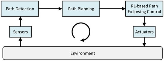
Figure 1. The action loop for the considered path following control task.

Reinforcement learning agents in simulation-based environments are usually trained with fixed model parameter values. In autonomous driving, however, some vehicle dynamics parameters might be uncertain or might change over time due to environmental influence. This might negatively affect the agents’ performance during their execution if the parameters cannot be determined beforehand or change after training. Figure 2 qualitatively shows this for a path-following motion control task. Let $\xi$ represent the dynamics parameter of the vehicle model. Furthermore, assume that ${\xi }_{\mathrm{train}}$ is a fixed value for $\xi$ that is applied to the vehicle learning model during training. On the left side of Figure 2, it can be seen that the agent performs well after training and during execution if the actual parameter ${\xi }_1$ of the vehicle equals the parameter ${\xi }_{\mathrm{train}}$. However, on the right side, the agent is not able to provide a satisfying control performance during execution and drives off the road since the true parameter ${\xi }_2$ of the vehicle differs from the fixed value ${\xi }_{\mathrm{train}}$ used during training. The possibility of such an unrobust control behavior poses a major security risk.

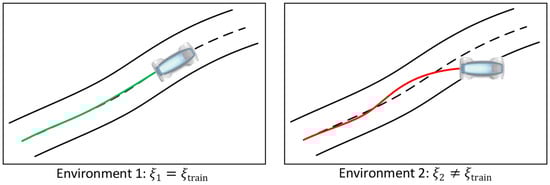
Figure 2. The performance of agents during execution for different values of a representative dynamics parameter $\xi$. (Left): The true parameter ${\xi }_1$ of the vehicle in the first environment equals the value ${\xi }_{\mathrm{train}}$ applied during the simulation-based training and the agent shows a satisfying path following control performance. (Right): The actual vehicle parameter ${\xi }_2$ in the second environment differs from ${\xi }_{\mathrm{train}}$ and the agent shows a poor path following control performance.

To overcome this issue and train robust agents for a path-following control task in the presence of uncertain and changing dynamics parameters, we apply dynamics randomization during the reinforcement learning process in this work. The underlying path following control problem considered in this paper is based on our previous work in [14] and is introduced in detail in Appendix A. We assume that the path boundaries can be detected in each time step and that a path planning module, such as in [15], is given. Furthermore, the learning model of the controlled vehicle is based on the extended non-linear single-track model of the ROboMObil [12] (c.f. Appendix B). We assume that a nonlinear observer, such as in [16], estimates the necessary states for the reinforcement learning controller.

3. Learning-Based Path following Control with Parametric Uncertainties

In deep reinforcement learning [17], a neural network represents the agent and interacts with an environment, receiving a reward in each time step. Here, the reward encodes the control goal. Based on the observed state of the environment, the agent applies an action and obtains a reward. The agent learns to solve a predefined control task by maximizing the expected sum of rewards in the environment. For the interested reader, the fundamentals of deep reinforcement learning are introduced in more detail in Appendix C. In this section, we introduce the observation space of the environment, the action space of the agent, and the reward function design for the path following control task at hand. Furthermore, the dynamics randomization scheme is presented.

3.1. Oberservation Space of the Path following Control Environment

The agents trained for the path following control task should minimize certain errors between the ROboMObil and the path, which is assumed to be provided by the ROboMObil’s path planning module [15,18]. More specifically, the agents should minimize the vehicle’s lateral position error $e_y^{\mathrm{P}}$ and orientation error $e_{\psi }$ to the path. Furthermore, the agents should closely track the demanded velocity in the tangential direction of the path, i.e., minimize the velocity error $e_{v_x}^{\mathrm{P}}$ (cf. Appendix A).

To successfully minimize these errors and learn the control task, the agents require a suitable observation space during training that contains all the necessary information regarding the environment. In this work, the observation vector $s_k$, also called the state, is chosen based on our previous work in [14]. Here, the aforementioned errors $e_y^{\mathrm{P}}, e_{\psi }$ and $e_{v_x}^{\mathrm{P}}$ as well as the velocity error $e_{v_y}^{\mathrm{P}}$ in the lateral direction of the path (cf. Appendix A), are provided for the observation vector. Furthermore, the path curvature ${\kappa }_{\mathrm{P}}$ and the front and rear steering angles ${\delta }^{\mathrm{f}}$ and ${\delta }^{\mathrm{r}}$ of the ROboMObil are incorporated into the observation vector $s_k$. Lastly, the observation vector $s_k$ in the time step $k$ is extended with the observation ${\sigma }_{k-1}$ of the aforementioned values from the previous time step $k-1$, which incorporates beneficial rate information into the learning process. This leads to the observation vector $s_k$ being

$${\mathbf{s}}_k=\left[e_{y,k}^{\mathrm{P}},e_{v_x,k}^{\mathrm{P}},e_{v_y,k}^{\mathrm{P}},e_{\psi ,k},{\kappa }_{\mathrm{P},k},{\delta }_k^{\mathrm{f}},{\delta }_k^{\mathrm{r}}, {\mathbf{\sigma }}_{k-1}\right]$$

(1)

with

$${\mathbf{\sigma }}_{k-1}=\left[e_{y,k-1}^{\mathrm{P}},e_{v_x,k-1}^{\mathrm{P}},e_{v_y,k-1}^{\mathrm{P}},e_{\psi ,k-1},{\kappa }_{\mathrm{P},k-1},{\delta }_{k-1}^{\mathrm{f}},{\delta }_{k-1}^{\mathrm{r}}\right].$$

(2)

3.2. Action Space of the Agents

The control inputs the agent can apply to the extended non-linear single-track model of the ROboMObil [12] are the front and rear axle steering rates ${\dot{\delta }}_{\mathrm{f}}$ and ${\dot{\delta }}_{\mathrm{r}}$ and the front and rear in-wheel torques ${\tau }_{\mathrm{f}}$ and ${\tau }_{\mathrm{r}}$, respectively. Both steering rates ${\dot{\delta }}_{\mathrm{f}}$ and ${\dot{\delta }}_{\mathrm{r}}$ are limited by the maximal steering rate ${\dot{\delta }}_{\max }$:

$$-{\dot{\delta }}_{\max }\le {\dot{\delta }}_i\le {\dot{\delta }}_{\max } \forall i \mathrm{in} \left\{\mathrm{f},\mathrm{r}\right\}.$$

(3)

Besides providing the steering rates to the vehicle, the agent also commands the front and rear in-wheel torques ${\tau }_{\mathrm{f}}$ and ${\tau }_{\mathrm{r}}$. The torques are limited by the maximum torque ${\tau }_{\max }$:

$$-{\tau }_{\max }\le {\tau }_i\le {\tau }_{\max } \forall i \mathrm{in} \left\{\mathrm{f},\mathrm{r}\right\}.$$

(4)

3.3. Design of the Reward Function

The design of the reward function provides a crucial degree of freedom in reinforcement learning. As mentioned above, the agent should be rewarded positively when it approaches the control goal, i.e., when it has small or no errors to the path. For the path-following control task, the agent should learn to control the vehicle such that the lateral offset $e_y^{\mathrm{P}}$, the orientation error $e_{\psi }$ and the velocity errors $e_{v_x}^{\mathrm{P}}$ are minimized. However, as mentioned in [14], the agent’s primary control goal should be to minimize the lateral position error $e_y^{\mathrm{P}}$, since a large lateral offset could negatively influence safety and possibly cause collisions. After minimizing the lateral position error, the agent should learn to control the vehicle such that it achieves the commanded orientations and velocities and both $e_{\psi }^{\mathrm{P}}$ and $e_{v_x}^{\mathrm{P}}$ approach zero. Furthermore, smooth steering behavior should be favored. Therefore, a hierarchical structure for the reward function is chosen, as in [14]. More specifically, the reward function is set to

$$r_{\mathrm{PFC}}\left(e_y^{\mathrm{P}},e_{\psi }^{\mathrm{P}},e_{v_x}^{\mathrm{P}},\mathsf{\Delta }{\delta }_{\mathrm{f}},\mathsf{\Delta }{\delta }_{\mathrm{r}}\right)=g_{{\mathbf{\theta }}_y}\left(e_y^{\mathrm{P}}\right)\left(1+r_e\left(e_{\psi }^{\mathrm{P}},e_{v_x}^{\mathrm{P}}\right)\left(1+r_{\mathsf{\Delta }\mathsf{\delta }}\left(\mathsf{\Delta }{\delta }_{\mathrm{f}},\mathsf{\Delta }{\delta }_{\mathrm{r}}\right)\right)\right)$$

(5)

with $r_e\left(e_{\psi }^{\mathrm{P}},e_{v_x}^{\mathrm{P}}\right)$ being

$$r_e\left(e_{\psi }^{\mathrm{P}},e_{v_x}^{\mathrm{P}}\right)=g_{{\mathbf{\theta }}_{\psi }}\left(e_{\psi }^{\mathrm{P}}\right)+g_{{\theta }_{v_x}}\left(e_{v_x}^{\mathrm{P}}\right)$$

(6)

and $r_{\mathsf{\Delta }\mathsf{\delta }}\left(\mathsf{\Delta }{\delta }_{\mathrm{f}},\mathsf{\Delta }{\delta }_{\mathrm{r}}\right)$ being

$$r_{\mathsf{\Delta }\mathsf{\delta }}\left(\mathsf{\Delta }{\delta }_{\mathrm{f}},\mathsf{\Delta }{\delta }_{\mathrm{r}}\right)=\frac{1}{1+c_{\mathrm{f}}\left|\mathsf{\Delta }{\delta }_{\mathrm{f}}\right|+c_{\mathrm{r}}\left|\mathsf{\Delta }{\delta }_{\mathrm{r}}\right|}.$$

(7)

Here, the expressions $\mathsf{\Delta }{\delta }_{\mathrm{f}}$ and $\mathsf{\Delta }{\delta }_{\mathrm{r}}$ denote the changes of the front and rear steering angles between the two subsequent time steps $k$ and $k-1$ which are given by

$$\begin{array}{c}\mathsf{\Delta }{\delta }_{\mathrm{f}}={\delta }_{\mathrm{f},k}-{\delta }_{\mathrm{f},k-1} \\ \mathsf{\Delta }{\delta }_{\mathrm{r}}={\delta }_{\mathrm{r},k}-{\delta }_{\mathrm{r},k-1}.\end{array}$$

(8)

Furthermore, $c_{\mathrm{f}}$ and $c_{\mathrm{r}}$ represent their weighting parameters in (7) and are set manually.

In Equations (5) and (6), the functions $g_{\mathbf{\theta }}\left(x\right)$ are Gaussian-like functions

$$g_{\mathbf{\theta }}\left(x\right)={\theta }_1{e}^{\frac{-x^2}{2{\theta }_2}}$$

(9)

with the properties

$$0<g_{\mathbf{\theta }}\left(x\right)\le {\theta }_1,\forall x\in ℝ,\forall \mathbf{\theta }=\left[{\theta }_1,{\theta }_2\right]\in {ℝ}_{+}^2.$$

(10)

For the reward $r_{\mathrm{PFC}}\left(e_y^{\mathrm{P}},e_{\psi }^{\mathrm{P}},e_{v_x}^{\mathrm{P}},\mathsf{\Delta }{\delta }_{\mathrm{f}},\mathsf{\Delta }{\delta }_{\mathrm{r}}\right)$ in Equation (5), the function $g_{{\mathbf{\theta }}_y}\left(e_y^{\mathrm{P}}\right)$ approaches zero for large lateral position errors $e_y^{\mathrm{P}}$ and approaches ${\theta }_{y,1}>0$ for small $e_y^{\mathrm{P}}$. Hence, the agent is rewarded for small lateral position errors. This term dominates the overall reward, since it is the only term multiplied by one (cf. Equation (5)), which is in-line with the hierarchical reward structure of prioritizing the minimization of the lateral position error first [14]. Furthermore, the value of $g_{{\mathbf{\theta }}_y}\left(e_y^{\mathrm{P}}\right)$ is multiplied by the reward term $r_e\left(e_{\psi }^{\mathrm{P}},e_{v_x}^{\mathrm{P}}\right)$ consisting of the Gaussian-like functions $g_{{\mathbf{\theta }}_{\psi }}\left(e_{\psi }^{\mathrm{P}}\right)$ and $g_{{\mathbf{\theta }}_{v_x}}\left(e_{v_x}^{\mathrm{P}}\right)$ (cf. Equation (6)) for the orientation and velocity errors $e_{\psi }^{\mathrm{P}}$ and $e_{v_x}^{\mathrm{P}}$ in Equation (5), which can further increase the overall reward $r_{\mathrm{PFC}}\left(e_y^{\mathrm{P}},e_{\psi }^{\mathrm{P}},e_{v_x}^{\mathrm{P}},\mathsf{\Delta }{\delta }_{\mathrm{f}},\mathsf{\Delta }{\delta }_{\mathrm{r}}\right)$ once the agent has successfully learned to minimize $e_y^{\mathrm{P}}$, i.e., maximize the function $g_{{\mathbf{\theta }}_y}\left(e_y^{\mathrm{P}}\right)$. Finally, after minimizing the lateral position error $e_y^{\mathrm{P}}$, the orientation error $e_{\psi }^{\mathrm{P}}$, and the velocity error $e_{v_x}^{\mathrm{P}}$, the agent receives a further reward determined by $r_{\mathsf{\Delta }\mathsf{\delta }}\left(\mathsf{\Delta }{\delta }_{\mathrm{f}},\mathsf{\Delta }{\delta }_{\mathrm{r}}\right)$ if it controls the vehicle such that there is a small steering rate between two subsequent time steps to favor smooth control of the vehicle.

3.4. Learning with Dynamics Randomization

Dynamics randomization [8,9,10] allows robust policies to be trained in cases where dynamics parameters are uncertain, difficult to measure, or frequently change over time. When dynamics randomization is applied, the dynamics parameters are sampled from a specific distribution at the beginning of each training episode. Figure 3 depicts this for a representative parameter $\xi$. Often, a uniform distribution $\mathcal{U}\left(a, b\right)$ within a predefined parameter range between the values $a$ and $b$ is chosen [8]. This enables the agent to learn a successful control performance for the entire uniformly distributed parameter range without favoring specific parameter values. In [8] it was shown that dynamics randomization can be interpreted as a trade-off between optimality and robustness. Therefore, the ranges in which the parameters are randomized need to be thoughtfully chosen to prevent the agents from learning overly conservative control behaviors.

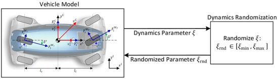
Figure 3. Dynamics randomization scheme at the beginning of each training episode for a representative dynamics parameter $\xi$. First, the parameter $\xi$ which should be randomized is selected and forwarded to the dynamics randomization module (top arrow). Afterwards, the randomized value ${\xi }_{\mathrm{rnd}}$ of the parameter $\xi$ is returned to the vehicle model (bottom arrow).

In this work, three agents are trained, whereby each agent experiences randomization for a different parameter of the vehicle model. More specifically, the parameters that are being randomized are the vehicle mass $m$, the yaw inertia $J_z^{\mathrm{C}}$ of the vehicle, and the tire-road friction coefficient $\mu$ (cf. Appendix B), which are often randomized in such setups [8,9]. More specifically, in this work, these particular randomizations are considered for the path-following control task based on the following reasons: the overall system mass changes every time a different load is placed inside the vehicle and also depends on whether a passenger is onboard. The inertia value is often difficult to measure and can be only estimated roughly. Furthermore, the tire-road friction frequently changes depending on the current weather.

Besides training the three agents experiencing dynamics randomization, an agent with the nominal vehicle dynamics parameters is also trained for the same PFC task, which serves as a benchmark. To allow a straightforward comparison, the agents experiencing randomization are set to have the same reward as well as the same action and observation spaces as the nominal agent experiencing no randomization. The different ranges of the uniform distributions $\mathcal{U}\left(a,b\right)$ in which the vehicle mass $m$, the yaw inertia $J_z^{\mathrm{C}}$ and the tire friction $\mu$ are randomized are introduced in the following.

3.4.1. Mass Randomization

The first agent being trained with dynamics randomization experiences randomization for the vehicle mass. The ROboMObil’s nominal mass is $m_{\mathrm{ROMO}}=1013 \mathrm{kg}$. The ROboMObil can either transport no passengers, a maximum of one passenger, or a certain amount of load, leading to an unknown external load that might be placed in the vehicle after training. Therefore, an external mass $m_{\mathrm{ext}}$ from a uniform distribution that covers all three application cases is sampled and added to the ROboMObil’s mass, which enables the agent to learn an equally successful control performance for the entire parameter range. This leads to the randomized training mass $m_{\mathrm{rnd}}$ being

$$m_{\mathrm{rnd}}=m_{\mathrm{ROMO}}+m_{\mathrm{ext}}.$$

(11)

At the beginning of each episode, after sampling $m_{\mathrm{ext}}$ and adding it to $m_{\mathrm{ROMO}}$, the randomized training mass $m_{\mathrm{rnd}}$ substitutes the vehicle model’s nominal mass $m_{\mathrm{ROMO}}$. In this work, the uniformly sampled external mass $m_{\mathrm{ext}}$ takes a value within the range

$$0 \mathrm{kg}\le m_{\mathrm{ext}}\le 300 \mathrm{kg}$$

(12)

3.4.2. Inertia Randomization

The second agent experiences randomization in the yaw inertia. The nominal yaw inertia value for the ROboMObil is $J_{z,\mathrm{nom}}^{\mathrm{C}}=1130 {\mathrm{kgm}}^2$. Since this is an estimated value, we assume that it has a significant amount of uncertainty within a $\pm 20 \%$ range of the nominal inertia value. Therefore, a randomized inertia value $J_{z,\mathrm{rnd}}^{\mathrm{C}}$ within the interval

$$\left(1-0.2\right)J_{z,\mathrm{nom}}^{\mathrm{C}}\le J_{z,\mathrm{rnd}}^{\mathrm{C}}\le \left(1+0.2\right)J_{z,\mathrm{nom}}^{\mathrm{C}}$$

(13)

is sampled beginning with every training episode to enable the agent to learn a successful control performance for the entire range of possible inertia values.

3.4.3. Friction Randomization

The third agent being trained with dynamics randomization experiences randomization for the road-tire friction. By varying the friction during training, the agent has the opportunity to learn how to control the vehicle robustly in various street conditions, such as on a dry surface, a wet surface, or a surface covered in snow. The friction has a proportional influence on the front and rear side wheel forces (cf. Equation (A14) of Pacejka’s Magic Formula (MF) [19] for the side wheel forces in Appendix B). The influence of different friction values on the side wheel forces is demonstrated in Figure 4. Here, the friction coefficient $\mu =1.0$ represents a dry, $\mu =0.8$ a wet, and $\mu =0.6$ a snowy road. It can be seen that, with decreasing friction $\mu$, the maximal lateral tire forces also decrease. This drastically influences the vehicle’s dynamic behavior and, consequently, affects the control performance.

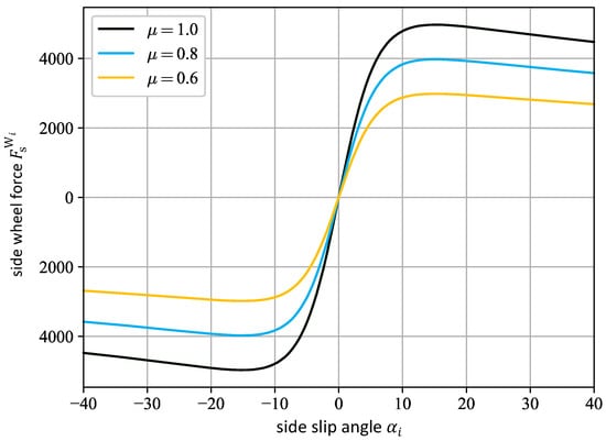
Figure 4. The side wheel forces $F_{\mathrm{s}}^{{\mathrm{W}}_i}$ over the side slip angle ${\alpha }_i$ for different values of $\mu$ with $i\in \left\{\mathrm{f},\mathrm{r}\right\}$ denoting the front or rear wheels, respectively, according to Pajecka’s MF [18] in Equation (A14).

To enable the agent to learn an equally robust and successful vehicle control strategy for different street conditions, a uniformly sampled friction value ${\mu }_{\mathrm{rnd}}$ within the range

$$0.6\le {\mu }_{\mathrm{rnd}}\le 1$$

(14)

is selected at the beginning of each episode. This friction value is afterwards used in the vehicle model during a training episode.

4. Training Setup

In this section, the simulation framework of the training setup, including the dynamics randomization process, is introduced. Furthermore, the training procedure for the agents is presented.

4.1. Simulation Framework

The software architecture applied to train the different agents with dynamics randomization is extended from our previous work in [14] and shown in Figure 5.

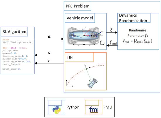
Figure 5. Training setup of the PFC task including dynamics randomization extended from [14].

Here, the reinforcement learning environment for the PFC problem is implemented using the Python-based OpenAI Gym framework [20]. This framework offers a standardized interface with several reinforcement learning libraries, such as the Stable-Baselines 2 library [21], used in this work. The vehicle model is written in Python as a system of ordinary differential equations (ODEs) and solved by the odeint-function from the Scipy library [22]. Furthermore, time independent path interpolation (TIPI) [12,23] is applied to determine the closest point on the reference path for each time step, which is then used by the agent to learn how to steer the vehicle towards the path. The implementation details of the TIPI are shown in Appendix A. The TIPI is implemented in Modelica [24] and exported by Dymola as a Functional Mock-up Unit (FMU) [25], which contains the compiled code of the TIPI algorithm. This FMU is then incorporated into the Python-based reinforcement learning framework.

4.2. Training Procedure

The agents are trained on the path depicted in Figure 6, which represents a federal highway called “Kesselberg”, located in the German Alps, and is parameterized by the arc length $s$. The corresponding desired velocity profile $v_{\mathrm{P}}^{\mathrm{I}}\left(s\right)$ is shown in Figure 7, calculated by taking the path curvature and the vehicle’s acceleration limits into account [26]. This particular path is chosen for training since it consists of road sections with different characteristics, which are beneficial for learning the RL-based PFC. In Figure 6 and Figure 7, for example, it can be seen that the path demands tight turns between the arc lengths $s=300 \mathrm{m}$ and $s=600 \mathrm{m}$ (cf. Figure 6) with a rather slow velocity around $v_{\mathrm{P}}^{\mathrm{I}}\left(s\right)=10 \raisebox{1ex}{$\mathrm{m}$}\!\left/ \!\raisebox{-1ex}{$\mathrm{s}$}\right.$ (cf. Figure 7). On the other hand, the path section between $s=900 \mathrm{m}$ and $s=1200 \mathrm{m}$ represents an almost straight road, where the vehicle needs to accelerate quickly to successfully track the velocity demanded. All agents are trained for a total of $300.000$ time steps with a step size of $\Delta t=0.05 \mathrm{s}$, and the reward function introduced in Equation (5). In this work, an episode consists of $300$ time steps. During training, we apply the state-of-the-art Soft Actor-Critic (SAC) [27] learning algorithm from the Stable-Baselines 2 library [21]. The SAC algorithm is briefly discussed in Appendix C. The training with the SAC method is conducted with the hyperparameters given in Appendix D. The parameters of the reward function introduced in Equation (5) are set to:

$${\mathbf{\theta }}_y=\left[1, 0.05\right],{\mathbf{\theta }}_{\psi }=\left[1, \sqrt{0.005}\right], {\mathbf{\theta }}_v=\left[1, \sqrt{0.1}\right].$$

(15)

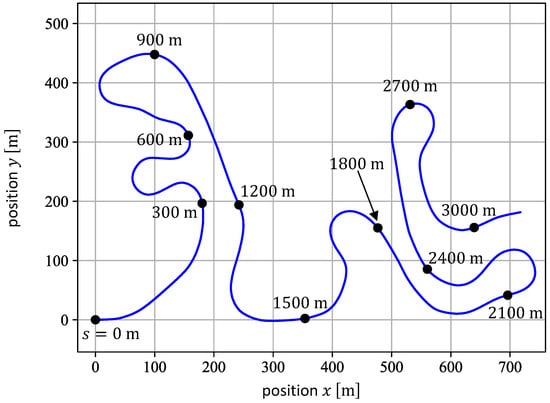
Figure 6. Top view of the training path (blue line), which represents a federal highway located in the German Alps. The black dots depict different path position at certain arc lengths $s$ [14].

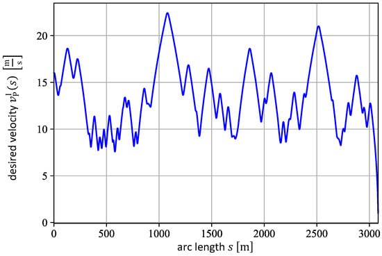
Figure 7. Velocity profile $v_{\mathrm{P}}^{\mathrm{I}}\left(s\right)$ of the training path, parameterized by the arc length $s$ [14].

Furthermore, the weighting parameters $c_{\mathrm{f}}$ and $c_{\mathrm{r}}$ in Equation (7) are both set to $1$ to equally penalize large changes in both the front and rear steering angles.

As introduced in [14], it is beneficial to randomly initialize the system with an offset to the path at the beginning of each training episode. This supports the exploration of the observation space since the agents must repeatedly try to successfully follow the path starting from different initial configurations. More specifically, the offset is applied to the initial position error $e_{y,\mathrm{start}}^{\mathrm{P}}$, the initial orientation error $e_{\psi ,\mathrm{start}}$, and the initial longitudinal velocity error $e_{v_x,\mathrm{start}}^{\mathrm{P}}$. At the beginning of each episode, these initial errors to the path are randomly sampled from three different uniform distributions within the following bounds:

$$\begin{array}{c}-0.8 \mathrm{m}\le e_{y,\mathrm{start}}^{\mathrm{P}}\le 0.8 \mathrm{m} \\ -8.6°\le e_{\psi ,\mathrm{start}}\le 8.6°\\ -1.0 \frac{\mathrm{m}}{\mathrm{s}}\le e_{v,\mathrm{start}}^{\mathrm{P}}\le 1.0 \frac{\mathrm{m}}{\mathrm{s}}.\end{array}$$

(16)

To further encourage the agents to only explore important parts of the observation space, several training abortion criteria are introduced, as described in [14]. If one or more of these errors do not remain within their respective pre-defined thresholds, then the training episode is terminated early. In this work, a termination is triggered in the following cases:

$$\left|e_y^{\mathrm{P}}\right|>2 \mathrm{m},\left|e_{\psi }\right|>70°, \left|e_{v_x}^{\mathrm{P}}\right|>5 \frac{\mathrm{m}}{\mathrm{s}}, \left|e_{v_y}^{\mathrm{P}}\right|>5 \frac{\mathrm{m}}{\mathrm{s}}.$$

(17)

Every time an episode is terminated, the negative terminal reward $r_{\mathrm{T}}=-10$ is provoked. Therefore, the agents need to learn to stay within these error thresholds, since a negative reward contradicts the primary reinforcement learning goal of maximizing the expected sum of rewards, also called the return $G$ (cf. Equation (A17) in Appendix C). When a new episode starts, the vehicle is reinitialized where the previous episode ended, with an initial offset according to Equation (16).

5. Tests and Performance Comparison

The agent trained with fixed nominal values (nomRL-PFC) is compared separately to the three agents trained with dynamics randomization. The agents are compared based on the returns they are able to achieve while facing changes in specific dynamics parameters during several executions on the path introduced in Figure 6. The return enables the direct comparison of the agents with respect to the control goal, since all agents had to learn how to maximize the same reward function during training. First, the nomRL-PFC is compared with the agent trained with randomized mass ($m$-randRL-PFC), followed by a comparison with the agent trained with randomized inertia ($J$-randRL-PFC). Lastly, the nomRL-PFC is compared with the agent trained with a randomized friction coefficient ($\mu$-randRL-PFC).

5.1. Tests and Comparison of the nomRL-PFC and the $m$-randRL-PFC

To evaluate the robustness and compare the performance of the nomRL-PFC and the $m$-randRL-PFC, both agents are executed several times on the path in Figure 6, where each time a different external mass $m_{\mathrm{ext}}$ is chosen within the interval $m_{\mathrm{ext}}\in \left[0 \mathrm{kg}, 300 \mathrm{kg}\right]$, i.e., the interval on which the agent with dynamics randomization was trained. The returns both agents obtained during these executions are shown in Figure 8. Here, the dark blue dot represents the return of the nomRL-PFC for the external mass $m_{\mathrm{ext}}=0 \mathrm{kg}$. The light-blue dashed line with the crosses represents the nominal agent’s returns for executions on the path that were aborted due to early termination (cf. Inequalities (17)). The orange line shows the return of the $m$-randRL-PFC for all external masses $m_{\mathrm{ext}}$.

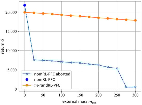
Figure 8. Return of the normRL-PFC (blue line) and $m$-randRL-PFC (orange line) after executions on the path for different external mass values $m_{\mathrm{ext}}$.

In Figure 8, it can be seen that the nomRL-PFC achieves a $9 \%$ higher return than the $m$-randRL-PFC for $m_{\mathrm{ext}}=0 \mathrm{kg}$, which is the value for which the nomRL-PFC was trained. However, the $m$-randRL-PFC outperforms the nominal agent for cases in which $m_{\mathrm{ext}}\ge 25 \mathrm{kg}$. In all cases with an additional mass, the execution of the nominal agent on the path is aborted early because it triggers one or more of the safety-critical termination conditions introduced in Equation (17). In the case of $m_{\mathrm{ext}}=300 \mathrm{kg}$, for example, the execution of the nomRL-PFC is aborted because the position error exceeds the respective pre-defined threshold, i.e., $\left|e_y^{\mathrm{P}}\right|>2 \mathrm{m}$ (cf. Inequalities (17)). This is illustrated in Figure 9. Here, the pathway of the nominal agent is depicted in blue, while the pathway of the $m$-randRL-PFC is depicted in orange. The reference path is presented by the dashed black line. The solid black lines represent the path boundaries. It can be observed that the nomRL-PFC starts to slightly deviate from the reference path until the agent eventually leaves the road. However, the $m$-randRL-PFC continues to successfully follow the path closely. Furthermore, for the complete interval of the values considered for $m_{\mathrm{ext}}$, the returns of the $m$-randRL-PFC remain at a relatively high level compared with the nomRL-PFC’s returns, which decrease continually. This underlines the robustness of the $m$-randRL-PFC against varying mass values.

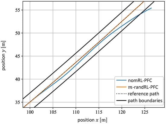
Figure 9. The pathways of the nomRL-PFC (blue line) and the m-randRL-PFC (orange line) for $m_{\mathrm{ext}}=300 \mathrm{kg}$. The reference path is depicted by the dashed black line, whereas the road boundaries are represented by the solid black lines.

Table 1 shows the root mean square error (RMS) of the lateral position, velocity, and orientation errors $e_y^{\mathrm{P}}$, $e_{v_x}^{\mathrm{P}}$, and $e_{\psi }^{\mathrm{P}}$ of the nomRL-PFC and the 𝑚-randRL-PFC during their execution along the entire path with $\Delta k=0.05 \mathrm{s}$. More specifically, we consider the cases $m_{\mathrm{ext}}=0 \mathrm{kg}$ and $m_{\mathrm{ext}}=300 \mathrm{kg}$, which represent both ends of the randomization interval. The errors of the nomRL-PFC are not provided for $m_{\mathrm{ext}}=300 \mathrm{kg}$ since the agent on the path failed to completely execute due to the early termination criteria described above. For $m_{\mathrm{ext}}=0 \mathrm{kg}$, the lateral position error $e_y^{\mathrm{P}}$-RMS of the nomRL-PFC is higher than that of the 𝑚-randRL-PFC. However, the nominal agent achieves a smaller RMS for both the velocity error $e_{v_x}^{\mathrm{P}}$ and the orientation error $e_{\psi }^{\mathrm{P}}$. In summary, the nomRL-PFC is able to achieve a higher overall return for $m_{\mathrm{ext}}=0 \mathrm{kg}$, as shown in Figure 8, resulting from the lower RMS of the velocity and orientation errors throughout the entire execution on the path. For $m_{\mathrm{ext}}=300 \mathrm{kg}$, the 𝑚-randRL-PFC’s returns decrease slightly compared with the case with $m_{\mathrm{ext}}=0 \mathrm{kg}$ because the RMS of all errors increases. This is the reason the return in Figure 8 also slightly decreases with higher values of $m_{\mathrm{ext}}$. Nevertheless, the 𝑚-randRL-PFC is able to achieve a high return for all values considered for the external mass $m_{\mathrm{ext}}$.

Table 1. The root mean square (RMS) errors of the nomRL-PFC and the $m$-randRL-PFC after executing the agents on the path for $m_{\mathrm{ext}}=0 \mathrm{kg}$ and $m_{\mathrm{ext}}=300 \mathrm{kg}$. The best metric for each $m_{\mathrm{ext}}$ value is marked green.

External Mass	${\mathit{m}}_{\mathbf{ext}}=0 \mathbf{kg}$		${\mathit{m}}_{\mathbf{ext}}=300 \mathbf{kg}$
Agent	nomRL-PFC	$\mathit{m}$-randRL-PFC	nomRL-PFC	$\mathit{m}$-randRL-PFC
$e_y^{\mathrm{P}} \left[\mathrm{m}\right]$ (RMS)	0.013	0.009	-	0.013
$e_{v_x}^{\mathrm{P}} \left[\raisebox{1ex}{$\mathrm{m}$}\!\left/ \!\raisebox{-1ex}{$\mathrm{s}$}\right.\right]$ (RMS)	0.106	0.149	-	0.594
$e_{\psi }^{\mathrm{P}} \left[\mathrm{rad}\right]$ (RMS)	0.020	0.032	-	0.033

Observing the results above, we can state that the 𝑚-randRL-PFC shows robustness against mass variations. This agent shows satisfying performances for the complete interval of $m_{\mathrm{ext}}$ ∈ [0 kg, 300 kg]. The performance of the nomRL-PFC, however, decreases drastically when the vehicle carries an external mass. This demonstrates that the nomRL-PFC agent is not robust against additional vehicle loads. Therefore, it fails to generalize to other parameter values that impose different dynamic behavior on the vehicle. Here, applying dynamics randomization to the mass during training solves this problem and enables the 𝑚-randRL-PFC to generalize successfully.

5.2. Tests and Comparison of the nomRL-PFC and the 𝐽-randRL-PFC

To examine the robustness of the nomRL-PFC and the 𝐽-randRL-PFC against variations in the yaw inertia, both agents are executed on the training path several times, where each time a different value for $J_{z,\mathrm{rnd}}^{\mathrm{C}}$ is chosen according to the inequalities (13). The returns of both agents are shown in Figure 10, which are evaluated at $80\%,85\%,\dots , 120\%$ of the nominal inertia value $J_{z,\mathrm{nom}}^{\mathrm{C}}$ of the ROboMObil. The blue line represents the returns of the nomRL-PFC, whereas the orange line depicts the returns of the 𝐽-randRL-PFC.

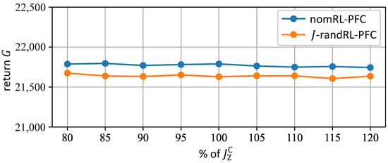
Figure 10. Return of the nomRL-PFC (blue line) and the 𝐽-randRL-PFC (orange line) for the inertia values considered during the training of the agent with dynamics randomization.

In Figure 10, it can be observed that the returns of the nomRL-PFC and the 𝐽-randRL-PFC both stay at a relatively constant level for all considered inertia values. The reason for this can be explained with the help of Table 2. It shows the RMS errors of the nomRL-PFC and the 𝐽-randRL-PFC for the inertia values $80\%\cdot J_{z,\mathrm{nom}}^{\mathrm{C}}$, $J_{z,\mathrm{nom}}^{\mathrm{C}}$ and $120\%\cdot J_{z,\mathrm{nom}}^{\mathrm{C}}$. The nomRL-PFC and the 𝐽-randRL-PFC each provide constant RMS errors for all three considered inertia values. Therefore, the returns of the agents do not vary notably. A possible explanation for this might be that the inertia does not have an overall major influence on the dynamics of the system for the considered motion control task, which is why the agents are able to perform equally well for all considered inertia values. Furthermore, both agents achieve similar RMS values for the position and orientation errors, with the nomRL-PFC providing slightly higher ones for both errors. For these errors, both agents receive similar overall rewards. Nevertheless, the nomRL-PFC is able to achieve higher overall returns in Figure 10 mainly due to the smaller RMS for the velocity error, which is rewarded higher due to the choice of ${\theta }_{v,2}$ in Equation (15).

Table 2. The root mean square (RMS) errors of the nomRL-PFC and the $J$-randRL-PFC after executing the agents on the path for different inertia values. The best metric for each inertia value is marked green.

Agent	nomRL-PFC			$\mathit{J}$-randRL-PFC
$\%\mathbf{of}\mathbf{Inertia}{\mathit{J}}_{\mathit{z},\mathbf{nom}}^{\mathbf{C}}$	$80\mathit{\%}$	$100\mathit{\%}$	$120\mathit{\%}$	$80\mathit{\%}$	$100\mathit{\%}$	$120\mathit{\%}$
$e_y^{\mathrm{P}} \left[\mathrm{m}\right]$ (RMS)	0.013	0.013	0.013	0.010	0.010	0.010
$e_{v_x}^{\mathrm{P}} \left[\raisebox{1ex}{$\mathrm{m}$}\!\left/ \!\raisebox{-1ex}{$\mathrm{s}$}\right.\right]$ (RMS)	0.106	0.106	0.106	0.144	0.144	0.144
$e_{\psi }^{\mathrm{P}} \left[\mathrm{rad}\right]$ (RMS)	0.020	0.020	0.020	0.013	0.014	0.014

With these observations, it can be stated that alternating the values of the yaw inertia does not affect the control performances of the agents. The RMS errors of both agents remain at a constant level, which indicates their robustness against different inertia values. More specifically, this shows that the nominal agent can still perform well even under uncertain inertia values and that the randomization of the yaw inertia during training does not provide any advantages.

5.3. Tests and Comparison of the nomRL-PFC and the $\mu$-randRL-PFC

To evaluate and compare the performance of nomRL-PFC and $\mu$-randRL-PFC for varying friction values, the agents both control the ROboMObil over the training path from start to finish multiple times, where each time a different tire-road friction coefficient $\mu$ is chosen. The performance of the agents is analyzed for friction values from the interval on which the $\mu$-randRL-PFC was trained; see Equation (14). The returns of both the nomRL-PFC and the $\mu$-randRL-PFC are shown in Figure 11 for several different friction values. The blue line represents the return of the nomRL-PFC, whereas the orange line depicts the return of the $\mu$-randRL-PFC. It can be seen that the nomRLPFC is able to obtain a higher return for friction values close to $\mu =1.0$, which is the friction value for which it was trained. However, for $\mu \le 0.925$, the nominal agent is outperformed by the $\mu$-randRL-PFC. Furthermore, the return of the nominal agent decreases significantly for smaller friction values, whereas the return of the agent trained with friction randomization is able to keep the return at a high level for all considered values of $\mu$, showing robust behavior on varying road conditions.

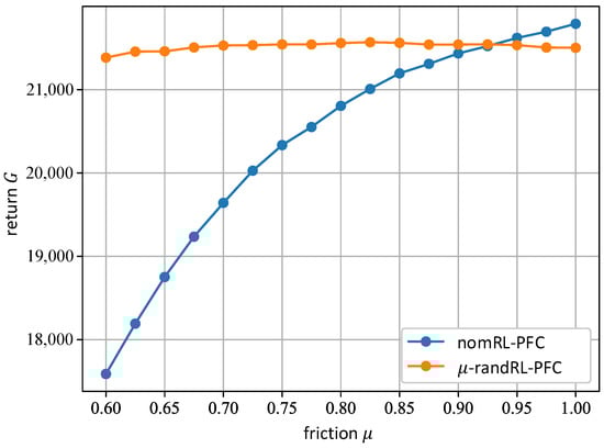
Figure 11. Return of the nomRL-PFC (blue line) and $\mu$-randRL-PFC (orange line) for the friction values considered during the training of the agent with dynamics randomization.

Table 3 summarizes the RMS errors of the nomRL-PFC and the $\mu$-randRL-PFC on the path for the friction values $\mu =0.6$ and $\mu =1.0$. It can be stated that both agents achieve a similar RMS for the lateral position error $e_y^{\mathrm{P}}$ on a dry road surface, i.e., $\mu =1.0$, with the nomRL-PFC providing lower errors for both velocity and orientation tracking. In the case of a snowy road with $\mu =0.6$, however, the path-following performance of the nomRL-PFC declines, which increases its RMS for $e_y^{\mathrm{P}}$ throughout the path. This is illustrated in Figure 12, which shows the road section around the arc length $s=493 \mathrm{m}$ for $\mu =0.6$, with the blue line depicting the pathway of the nomRL-PFC and the orange one illustrating the pathway of the $\mu$-randRL-PFC. It can be observed that both agents are able to successfully follow the reference path, while the $\mu$-randRL-PFC is able to achieve smaller lateral position errors to the reference path. This is the main reason why the overall return of the nomRL-PFC also decreases in Figure 11 for small friction values. The lateral position error $e_y^{\mathrm{P}}$ determines the value of the Gaussian-like function $g_{{\mathbf{\theta }}_y}\left(e_y^{\mathrm{P}}\right)$ in Equation (5), which is multiplied with the remainder of the reward function as part of the hierarchical design of the reward function. With increasing lateral position errors $e_y^{\mathrm{P}}$, the value of the function $g_{{\mathbf{\theta }}_y}\left(e_y^{\mathrm{P}}\right)$ decreases. Consequently, this leads to a smaller overall return during the execution on the path. The $\mu$-randRL-PFC, on the other hand, is able to obtain a similar $e_y^{\mathrm{P}}$-RMS for both road conditions (cf. Table 3), which further underlines its robustness against different friction values.

Table 3. The RMS errors of nomRL-PFC and $\mu$-randRL-PFC during the evaluation on the training path for the friction values $\mu =0.6$ and $\mu =1.0$. The best metric is highlighted green.

Friction Value	$\mathit{\mu }=0.6$		$\mathit{\mu }=1.0$
Agent	nomRL-PFC	$\mathit{\mu }$-randRL-PFC	nomRL-PFC	$\mathit{\mu }$-randRL-PFC
$e_y^{\mathrm{P}} \left[\mathrm{m}\right]$ (RMS)	0.033	0.011	0.013	0.013
$e_{v_x}^{\mathrm{P}} \left[\raisebox{1ex}{$\mathrm{m}$}\!\left/ \!\raisebox{-1ex}{$\mathrm{s}$}\right.\right]$ (RMS)	0.114	0.171	0.106	0.150
$e_{\psi }^{\mathrm{P}} \left[\mathrm{rad}\right]$ (RMS)	0.022	0.020	0.020	0.022

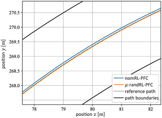
Figure 12. Pathways of the nomRL-PFC (blue lines) and the $\mu$-randRL-PFC (orange line) on the road section around the arc length $s=493 \mathrm{m}$ with the friction value $\mu =0.6$. The reference path is represented by the black dashed line, whereas the path boundaries are depicted by the black solid lines.

The performance comparison of the nomRL-PFC and the $\mu$-randRL-PFC at rather challenging road sections further demonstrates the robustness of the latter agent. The tight road turns between the arc lengths $s=300 \mathrm{m}$ and $s=600 \mathrm{m}$ of the path shown in Figure 6 represent such sections. The lateral position errors $e_y^{\mathrm{P}}$ induced by executing both agents in this particular part of the path are shown in Figure 13 for the friction value $\mu =1.0$, with the blue line representing the nomRL-PFC and the orange line representing the $\mu$-randRL-PFC. Here, it can be seen that both agents achieve a reasonable performance with the nomRL-PFC offering a slightly better one since it tracks the reference path more closely with $\left|e_y^{\mathrm{P}}\right|<0.024 \mathrm{m}$ in this section. However, the path-following performance of the nomRL-PFC in this part of the path decreases significantly for $\mu =0.6$, which can be seen in Figure 14. Here, it can be observed that the nomRL-PFC now makes greater position errors up to $\left|e_y^{\mathrm{P}}\right|\approx 0.06 \mathrm{m}$ and that it does not follow the path as closely as it did under dry road conditions ($\mu =1.0$). Furthermore, the $\mu$-randRL-PFC offers good position tracking performance with $\left|e_y^{\mathrm{P}}\right|<0.02 \mathrm{m}$ for $\mu =0.6$ (cf. Figure 14).

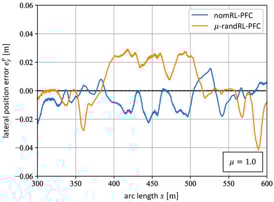
Figure 13. The position error $e_y^{\mathrm{P}}$ of the nomRL-PFC (blue line) and the $\mu$-randRL-PFC (orange line) on the road section between the arc lengths $s=300$ and $s=600$ for the friction value $\mu =1.0$.

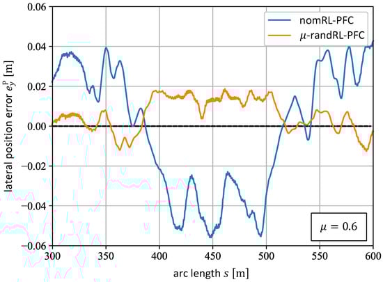
Figure 14. The position error $e_y^{\mathrm{P}}$ of the nomRL-PFC (blue line) and the $\mu$-randRL-PFC (orange line) on the road section between the arc lengths $s=300$ and $s=600$ for the friction value $\mu =0.6$.

Furthermore, in Table 3, it can be seen that the nomRL-PFC outperforms the $\mu$-randRL-PFC in terms of tracking the demanded velocity. For both friction values, the $\mu$-randRL-PFC generates a higher RMS of $e_{v_x}^{\mathrm{P}}$ over the entire path. This can be explained by the hierarchical design of the reward function. It prioritizes the minimization of the position error before rewarding small velocity errors. This prioritization motivates the $\mu$-randRL-PFC to apply a rather conservative velocity tracking performance for all friction values as a trade-off for good position tracking. Therefore, the agent trained with friction randomization applies a slower velocity for the different friction values in order to track the position more successfully for any given friction value $\mu \in \left[0.6, 1.0\right]$.

It can be stated that the randomization of the road-tire friction during training increases the robustness of the agent. The performance of the $\mu$-randRL-PFC stays at a high level, whereas the performance of the nomRL-PFC steadily decreases for smaller $\mu$.

6. Conclusions and Outlook

In this work, the reinforcement learning-based path-following control of the ROboMObil has been extended such that dynamics randomization can be applied during training, which enables the learning of robust agents. More specifically, the dynamics randomization method was applied to three different dynamics parameters of the ROboMObil, namely the vehicle mass, the yaw inertia, and the tire-road friction coefficient. In the case of mass randomization, the agent trained with uniformly distributed mass values showed superior performance for the entire range of additional loads, which underlines its robustness against variations in this particular vehicle parameter. In contrast, the nominal agent failed to complete the path-following control task with an additional vehicle load, which further displays the increased robustness of the former agent. Furthermore, the agent trained with randomized friction values performed impressively over all considered friction values, whereas the performance of the nominal agent declines continually under more slippery road conditions. This shows that randomizing the friction during training enables robust control performance for various road conditions. However, the nominal agent showed robustness against uncertainties in the yaw inertia, which reveals that the randomization of the inertia does not provide additional benefits. In summary, the results allow the conclusion that dynamics randomization for certain parameters that have a major impact on the vehicle dynamics, such as the mass and the friction, significantly increases the agents’ robustness against parametric uncertainties. In future work, an agent for the considered path-following control problem should be trained that experiences randomization in multiple parameters simultaneously. Furthermore, the performance of the agents should be validated experimentally in a real-world setup. However, appropriate safety measures need to be guaranteed first to ensure the safety of the system and the environment.

References

- Arnold, E.; Al-Jarrah, O.Y.; Dianati, M.; Fallah, S.; Oxtoby, D.; Mouzakitis, A. A Survey on 3D Object Detection Methods for Autonomous Driving Applications. IEEE Trans. Intell. Transp. Syst. 2019, 20, 3782–3795. [Google Scholar] [CrossRef]
- Yurtsever, E.; Lambert, J.; Carballo, A.; Takeda, K. A Survey of Autonomous Driving: Common Practices and Emerging Technologies. IEEE Access 2020, 8, 58443–58469. [Google Scholar] [CrossRef]
- Krasowski, H.; Wang, X.; Althoff, M. Safe Reinforcement Learning for Autonomous Lane Changing Using Set-Based Prediction. In Proceedings of the 2020 IEEE 23rd International Conference on Intelligent Transportation Systems (ITSC), Rhodes, Greece, 20–23 September 2020. [Google Scholar] [CrossRef]
- Wang, X.; Krasowski, H.; Althoff, M. CommonRoad-RL: A Configurable Reinforcement Learning Environment for Motion Planning of Autonomous Vehicles. In Proceedings of the 2021 IEEE International Intelligent Transportation Systems Conference (ITSC), Indianapolis, IN, USA, 19–22 September 2021. [Google Scholar] [CrossRef]
- Di, X.; Shi, R. A survey on autonomous vehicle control in the era of mixed-autonomy: From physics-based to AI-guided driving policy learning. Transp. Res. Part C Emerg. Technol. 2021, 125, 103008. [Google Scholar] [CrossRef]
- Kiran, B.R.; Sobh, I.; Talpaert, V.; Mannion, P.; Al Sallab, A.A.; Yogamani, S.; Perez, P. Deep Reinforcement Learning for Autonomous Driving: A Survey. IEEE Trans. Intell. Transp. Syst. 2022, 23, 4909–4926. [Google Scholar] [CrossRef]
- Pérez-Gil, Ó.; Barea, R.; López-Guillén, E.; Bergasa, L.M.; Gómez-Huélamo, C.; Gutiérrez, R.; Díaz-Díaz, A. Deep reinforcement learning based control for Autonomous Vehicles in CARLA. Multimed. Tools Appl. 2022, 81, 3553–3576. [Google Scholar] [CrossRef]
- Tan, J.; Zhang, T.; Coumans, E.; Iscen, A.; Bai, Y.; Hafner, D.; Bohez, S.; Vanhoucke, V. Sim-to-Real: Learning Agile Locomotion for Quadruped Robots. In Proceedings of the Robotics: Science and Systems XIV Conference, Pennsylvania, PA, USA, 26–30 June 2018; p. 10. [Google Scholar] [CrossRef]
- Bin Peng, X.; Andrychowicz, M.; Zaremba, W.; Abbeel, P. Sim-to-Real Transfer of Robotic Control with Dynamics Randomization. In Proceedings of the 2018 IEEE International Conference on Robotics and Automation (ICRA), Brisbane, Australia, 21–25 May 2018. [Google Scholar] [CrossRef]
- Antonova, R.; Cruciani, S.; Smith, C.; Kragic, D. Reinforcement Learning for Pivoting Task. arXiv 2017, arXiv:1703.00472. [Google Scholar] [CrossRef]
- Osinski, B.; Jakubowski, A.; Ziecina, P.; Milos, P.; Galias, C.; Homoceanu, S.; Michalewski, H. Simulation-Based Reinforcement Learning for Real-World Autonomous Driving. In Proceedings of the 2020 IEEE International Conference on Robotics and Automation (ICRA), Paris, France, 31 May–31 August 2020. [Google Scholar] [CrossRef]
- Brembeck, J. Model Based Energy Management and State Estimation for the Robotic Electric Vehicle ROboMObil. Dissertation Thesis, Technical University of Munich, Munich, Germany, 2018. [Google Scholar]
- Brembeck, J.; Ho, L.; Schaub, A.; Satzger, C.; Tobolar, J.; Bals, J.; Hirzinger, G. ROMO—The Robotic Electric Vehicle. In Proceedings of the 22nd IAVSD International Symposium on Dynamics of Vehicle on Roads and Tracks, Manchester, UK, 11–14 August 2011. [Google Scholar]
- Ultsch, J.; Brembeck, J.; De Castro, R. Learning-Based Path Following Control for an Over-Actuated Robotic Vehicle. In Autoreg 2019; VDI Verlag: Düsseldorf, Germany, 2019; pp. 25–46. [Google Scholar] [CrossRef]
- Winter, C.; Ritzer, P.; Brembeck, J. Experimental investigation of online path planning for electric vehicles. In Proceedings of the 2016 IEEE 19th International Conference on Intelligent Transportation Systems (ITSC), Rio de Janeiro, Brazil, 1–4 November 2016. [Google Scholar] [CrossRef]
- Brembeck, J. Nonlinear Constrained Moving Horizon Estimation Applied to Vehicle Position Estimation. Sensors 2019, 19, 2276. [Google Scholar] [CrossRef] [PubMed]
- Arulkumaran, K.; Deisenroth, M.P.; Brundage, M.; Bharath, A.A. Deep Reinforcement Learning: A Brief Survey. IEEE Signal Process. Mag. 2017, 34, 26–38. [Google Scholar] [CrossRef]
- Brembeck, J.; Winter, C. Real-time capable path planning for energy management systems in future vehicle architectures. In Proceedings of the 2014 IEEE Intelligent Vehicles Symposium, Dearborn, MI, USA, 8–11 June 2014. [Google Scholar] [CrossRef]
- Pacejka, H. Tire and Vehicle Dynamics, 3rd ed.; Butterworth-Heinemann: Oxford, UK, 2012. [Google Scholar]
- Brockman, G.; Cheung, V.; Pettersson, L.; Schneider, J.; Schulman, J.; Tang, J.; Zaremba, W. OpenAI Gym. arXiv 2016, arXiv:1606.01540. [Google Scholar]
- Hill, A.; Raffin, A.; Ernestus, M.; Gleave, A.; Kanervisto, A.; Traore, R.; Dhariwal, P.; Hesse, C.; Klimov, O.; Nichol, A.; et al. Stable Baselines. Available online: https://github.com/hill-a/stable-baselines (accessed on 15 December 2022).
- Virtanen, P.; Gommers, R.; Oliphant, T.; Haberland, M.; Reddy, T.; Cournapeau, D.; Burovski, E.; Peterson, P.; Weckesser, W.; Bright, J.; et al. SciPy 1.0 Contributors. SciPy 1.0 Fundamental Algorithms for Scientific Computing in Python. Nat. Methods 2020, 17, 261–272. [Google Scholar] [CrossRef] [PubMed]
- Ritzer, P.; Winter, C.; Brembeck, J. Advanced path following control of an overactuated robotic vehicle. In Proceedings of the 2015 IEEE Intelligent Vehicles Symposium (IV), Seoul, Republic of Korea, 28 June–1 July 2015. [Google Scholar] [CrossRef]
- Modelica Association. Modelica—A Unified Object-Oriented Language for Systems Modeling. Available online: https://modelica.org/documents/MLS.pdf (accessed on 13 January 2023).
- Modelica Association. Functional Mock-Up Interface. Available online: https://fmi-standard.org/ (accessed on 4 January 2023).
- Bünte, T.; Chrisofakis, E. A Driver Model for Virtual Drivetrain Endurance Testing. In Proceedings of the 8th International Modelica Conference, Dresden, Germany, 20–22 March 2011. [Google Scholar] [CrossRef]
- Haarnoja, T.; Zhou, A.; Abbeel, P.; Levine, S. Soft Actor-Critic: Off-Policy Maximum Entropy Deep Reinforcement Learning with a Stochastic Actor. In Proceedings of the 35th International Conference on Machine Learning, Stockholm, Sweden, 10–15 July 2018. [Google Scholar]
- Sutton, R.; Barto, A. Reinforcement Learning: An Introduction; A Bradford Book: Cambridge, MA, USA, 2018. [Google Scholar]
- Ziebart, B. Modeling Purposeful Adaptive Behavior with the Principle of Maximum Causal Entropy. Dissertation Thesis, Carnegie Mellon University, Pittsburgh, PA, USA, 2010. [Google Scholar]
Disclaimer/Publisher’s Note: The statements, opinions and data contained in all publications are solely those of the individual author(s) and contributor(s) and not of MDPI and/or the editor(s). MDPI and/or the editor(s) disclaim responsibility for any injury to people or property resulting from any ideas, methods, instructions or products referred to in the content. |
© 2023 by the authors. Licensee MDPI, Basel, Switzerland. This article is an open access article distributed under the terms and conditions of the Creative Commons Attribution (CC BY) license (https://creativecommons.org/licenses/by/4.0/).