HWACOA Scheduler: Hybrid Weighted Ant Colony Optimization Algorithm for Task Scheduling in Cloud Computing

Abstract

With the advancement of technology and time, people have always sought to solve problems in the most efficient and quickest way possible. Since the introduction of the cloud computing environment along with many different sub-substructures such as task schedulers, resource allocators, resource monitors, and others, various algorithms have been proposed to improve the performance of the individual unit or structure used in the cloud environment. The cloud is a vast virtual environment with the capability to solve any task provided by the user. Therefore, new algorithms are introduced with the aim to improve the process and consume less time to evaluate the process. One of the most important sections of cloud computing is that of the task scheduler, which is responsible for scheduling tasks to each of the virtual machines in such a way that the time taken to execute the process is less and the efficiency of the execution is high. Thus, this paper plans to propose an ideal and optimal task scheduling algorithm that is tested and compared with other existing algorithms in terms of efficiency, makespan, and cost parameters, that is, this paper tries to explain and solves the scheduling problem using an improved meta-heuristic algorithm called the Hybrid Weighted Ant Colony Optimization (HWACO) algorithm, which is an advanced form of the already present Ant Colony Optimization Algorithm. The outcomes found by using the proposed HWACO has more benefits, that is, the objective for reaching the convergence in a short period of time was accomplished; thus, the projected model outdid the other orthodox algorithms such as Ant Colony Optimization (ACO), Quantum-Based Avian Navigation Optimizer Algorithm (QANA), Modified-Transfer-Function-Based Binary Particle Swarm Optimization (MTF-BPSO), MIN-MIN Algorithm (MM), and First-Come-First-Serve (FCFS), making the proposed algorithm an optimal task scheduling algorithm.

1. Introduction

Since the time that cloud computing was introduced, almost all the data and tasks were handled by the cloud and, to assign each task to a particular virtual machine, a processor called the task scheduler was introduced, which, up to today, new algorithms have been proposed in order to enhance the performance of the task scheduler and also enhance the parameters involved. The main reason why we focus on the task scheduling component compared to other components is that task scheduling is one of the most essential and crucial parts, as it is responsible for assigning each of the virtual machines present in the cloud with the task requested by the user and returning the completed task back to the user. As mentioned before, various parameters and hyperparameters have been considered to establish a more enhanced task scheduler, some of which include the total cost of task execution, completion time, tolerance of faults, resource usage, and energy consumption. The procedure of scheduling tasks appears to be an NP complete problem, as the difficulty of the problem depends on the expanse of time taken to determine the solution, which may differ in different situations [1,2,3].

The main objective of the algorithm is to reduce the cost and time taken to execute the task while, at the same time, improving the performance of the task schedulers. The algorithm used for scheduling the task plays an important role in cloud computing, as it proficiently searches and makes decisions actively to determine the exact and apt virtual machine to execute each task. In order to arrive at an ideal and fine algorithm, various hyperparameters and parameters are used, such as makespan, time of response, utilization of the system, and network-based measures, which include the expenditure of the network communication, round trip, traffic volume, and many more. The method of finding the tasks available in the cloud can be characterized as a hybrid, heuristic, and meta-heuristic scheduling of task methods. There are algorithms where hybrid scheduling is used, and then there are some methods where a combination of heuristic and meta-heuristics approaches is used. In the algorithm where heuristic task scheduling is used, assigning the task is easy and often the quickest way to return the required outcome, but the ideal result is not guaranteed. When only taking into mind the time required for computation, algorithms using the meta-heuristic approach are better, as they attain a huge probing space to find the required result, thus decreasing the time required for computation. The area of concern now is the task scheduler, which is an important part, as it impacts the operation of cloud computing. Users such as creators and programmers, use common possessions due to the help of the cloud and, depending on the user’s needs and specifications, several different dedicated algorithms are recorded to aid the users in attaining the essential outcome [4,5].

Thus, a robust and efficient task scheduler algorithm is required that offers an ideal solution set. There is no problem seen while executing it on a simple system, but when executing it on a complex system, it should be able to handle enormous data and be able to complete the process. Nevertheless, during this process, there may be some problems encountered. Therefore, an efficient algorithm will be required to handle and process the data to obtain the required results.

Moreover, enumeration is needed to build a scheduler that is optimal, and, for this to happen, a process of building all task scheduling systems is required, that is, it mainly focuses on building a task structure from the already available set of tasks to get the related result set and cross check with each other to get an ideal set of solutions that can be used in the cloud environment for assigning each task to the correct virtual machine to improve the performance by minimizing the time consumed for handling a huge number of tasks. An algorithm tries to solve the scheduling-of-tasks problem by utilizing either a meta-heuristic or heuristic-based algorithm. The optimal result set that is considered ideal can be obtained by making use of a heuristic-based approach, as these approaches utilize some already defined rules, and results obtained by these programs vary based on the size of the problem and the underlying rules.

In addition to this, the meta-heuristic approach is used to solve extremely complex problems, as this approach generally makes use of a set of solutions to obtain the required solution space, which is completely different in terms of operation when compared to the functions used in the mathematical approach or the heuristic method, where only one candidate result space is used. Therefore, meta-heuristic-based algorithms perform better in comparison to the mathematical function and heuristic-based methods. Some of the famous algorithms used to solve the scheduling of task problem are the Quantum-Based Avian Navigation Optimizer Algorithm (QANA), the Modified-Transfer-Function-Based Binary Particle Swarm Optimization (MTF-BPSO), the Ant Colony Optimization (ACO), the MIN-MIN Optimization Algorithm (MM), and the First-Come-First-Serve Algorithm (FCFS).

In this paper, a new algorithm called the Hybrid Weighted Ant Colony Optimization Algorithm (HWACOA) is introduced that optimizes the process of task scheduling. The main objective of this program or method is to reduce the time taken for execution and the cost of operation. To summarize this paper:

o

In order to understand the problems faced by other task scheduling techniques and algorithms and to analyze how this affects the performance of the cloud, many various works have been reviewed.

o

Based on the understanding from the various works, this paper introduces a new innovative hybrid algorithm called the Hybrid Weighted Ant Colony Optimization Algorithm (HWACOA), which enhances the shortcomings and problems encountered by various different algorithms and, thus, improves the performance of scheduling the task.

o

Last but not the least, comparison between the results obtained by the introduced algorithm with many other algorithms has been conducted, and this was done by comparing extensive experimental simulation results obtained by various different algorithms using paired t-tests.

2. Related Works

All the resource allocation for the clients was done by the cloud service providers who first obtained the resources required for computing. In order to obtain efficient utilization of the resources, ideal task schedulers play an important role. In this work, RADL (Resource and Deadline Aware Dynamic Load balancer) for task scheduling in the cloud was introduced. The introduced task scheduler method evenly distributes the arriving work, which is considered to be computer-intensive and has a run time independent task. Moreover, the RADL algorithm has the ability to adjust the new incoming task effectively, and the task rejection is reduced. Experimental results obtained display that the introduced method attained up to 259.2%, 303.57%, 67.74%, 259.14%, 405.06% and 146.13% improvement for meeting task execution cost, tasks deadlines, meeting tasks deadlines, average resource utilization, penalty cost, and task response time, respectively, in comparison to the state-of-the-art heuristic scheduling of tasks using the benchmark datasets [6].

A huge volume of data means a large amount of data processing is required, and, due to this fact, the execution of the algorithm in the cloud environment becomes costly and consumes considerable energy. Many different algorithms have been introduced that try to search for the optimal result for scheduling workflow on the cloud, but there are some drawbacks in most of them. In this work, an EViMA (Energy Efficient Virtual Machine Mapping Algorithm) was introduced in order to enhance the management of the resources in the environment and to accomplish efficient task scheduling, which would reduce the data consuming energy, execution time, and cost. This algorithm is designed in such a way that it will meet all the necessities of the cloud user, and, at the same time, the quality of service is increased. In the introduced algorithm, the heterogenous properties of the scheduler from both workflow application user and cloud user were considered. By conducting experimental analysis on the real dataset, the introduced EViMA can give improved results for cloud providers and users by decreasing the makespan, cost, and consumption of energy [7].

As cloud computing offers various advantageous benefits, it attracts many entrepreneurs and IT leaders of various levels to use the cloud environment. Cloud computing makes use of many different technologies, such as mobile computing, the Internet of Things, and many more, out of which the task scheduler is one of the most important parts and is a challenging issue itself due to its NP-hard nature. Various methods have been introduced for ideal task scheduling that aim to improve the quality of service as well. This work tries to introduce a new Sailfish Optimization-based task Scheduling Algorithm (SOSA). SOSA was applied on two datasets, which showed a result of 7.81% and 13.71% which is an average improvement of performance in terms of makespan in comparison to Particle Swarm Optimization (PSO) and Genetic Algorithm (GA), respectively, and 30.78% and 11.30% of average improvement in terms of cost of execution in comparison to PSO and GA, respectively [8].

Due to the versatile nature of the cloud environment, which includes features such as fast and high accessibility, cheaper cost of operation, availability, and elasticity, the cloud computing environment has been utilized by researchers for the implementation of huge-scale task processing. Moreover, a pay-per-use charge is applied to each end user and, due to this factor, the efficiency is improved. The process of scheduling the work is difficult, as the processor in charge of executing this procedure needs to consider the dependence of the work in the environment along with the QoS (quality of service) demands. When there are many quality of service demands, the issue becomes more challenging. A lot of algorithms have been proposed in order to reduce the cost of execution and makespan under budget and deadline constraints. This paper introduces an algorithm for workflow scheduling which is based on java to reduce the makespan and execution cost to return a result in accordance with the weights provided by the end user. The introduced algorithm is compared with various other algorithms such as Round-Robin, MIN-MIN, Heterogenous Earliest Finish Time First, MAX-MIN, Dynamic Heterogenous Earliest Finish Time First, First-Come-First-Serve, and Minimum Completion Time in WorkFlowSim. The experimental results are compared based on both time and cost. The results obtained suggest that the introduced algorithm performs better when compared to other algorithms [9].

Edge computing is new method, which is closely related to the idea of the IoT (Internet of Things), as this method considers only those resources for computing that are essential in order to fulfil the user/consumer demand—that is, making use of the edge resourcing during computation, due to less bandwidth of the network being used and less time taken to respond, and, in order to achieve these goals, workflow scheduling must be taken into consideration. In this work, an improved version of the Firefly Algorithm, which is used to tackle the workflow scheduling challenge in the edge-based cloud environment, is introduced. The introduced algorithm overcame the deficiencies seen in the traditional meta-heuristic Firefly Algorithm by incorporating quasi-reflection-based learning methods and genetic operators. First, we checked the introduced method on 10 standard benchmark illustrations and made comparison of its performance with the traditional and other improved algorithms. Then, we performed experiments to generate a set of results for the scheduling of the workflow issue with two goals, which were the makespan and the cost. The algorithm introduced in this paper displayed vital improvement in comparison with the traditional Firefly Algorithm and meta-heuristic algorithms in terms of quality and speed of convergences [10].

The field of computing has seen a boost in its usage after the introduction of cloud computing, which has the capability of handling internet traffic and the various tasks requested by the end user. The cloud is made up of many different components, such as the resources manager, task manager, scheduler, and many more. In order to enhance the performance of the cloud, the performance of various components present in the cloud must be improved; as a result, many scholars have introduced various algorithms. Scheduler algorithms, to be more specific, have been introduced, as they provide a near optimal solution. This paper tries to introduce a new updated Sun Flower Optimization Algorithm to improve the task scheduler in terms of makespan and execution cost. The algorithm comprises two steps—movement and pollination—that suggest an ideal firmness among exploitation and exploration searches. The experimental stimulation obtained from the introduced algorithm was compared with various well-known algorithms, and it was seen that the introduced algorithm performed better in terms of makespan and cost of execution [11].

In this work, the proposed task scheduler algorithm—LPMSA (The Local Pollination-based Moth Search Algorithm)—is based on the hybridization of the Flower Pollination Algorithm (FPA) along with the Moth Search Algorithm (MSA). The introduced algorithm selects an ideal result for the correct scheduling of tasks in the cloud environment. In addition, the capacity of exploitation of the MSA is enhanced by making use of the local search technique as seen in the FPA algorithm. In this paper, a two-fold experimental simulation technique was used. The introduced algorithm LPMSA for scheduling of the task performance was evaluated based on the high and low heterogeneous machine with both non-uniformity and uniformity parameters. The experimental analysis showed that the introduced algorithm LPMSA had better performance in terms of consumption of energy and makespan [12].

One of the best features of the cloud computing environment is its ability to perform dynamic resource allocation; however, it experiences a major issue in terms of the quality of the service, consumption of energy, and fault tolerance. Hence, it was necessary to find an efficient algorithm which could effectively address these vital problems and improve the performance of the cloud. This paper introduces a dynamic-based resource allocator algorithm which could meet the user demands in terms of resources with a faster and improved responsiveness. It also presents a multi-object algorithm for searching called S-MOAL (Spacing Multi-Objective Antlion Algorithm) to reduce both the cost of usage of the VM (virtual machine) and the makespan. Moreover, its impact on the consumption of energy and tolerance to fault was also studied. The experimental result shows that the introduced algorithm performed better than DCLCA, PBACO, MOGA, DSOS and PBACO algorithms, especially in terms of makespan [13].

Herein, a study was conducted on the resource provisioning and scheduling of tasks in the cloud environment, and a conclusion was reached that stated that there was a prominent issue in the cloud environment due to its heterogeneity as well as the dispersion of the resources in the cloud environment. Due to the high demand for computation power, the cloud service providers are trying to build more data centers, but it is a threat to the environment in terms of the consumption of energy. To overcome these problems, a more effective meta-heuristic method is required that assigns application among the VMs (virtual machines) fairly, optimizes the QoS (quality of service), and meets the requirements of the end user. BPSO (Binary Particle Swarm Optimization) has been used to resolve real-world distinct optimization issues, but the BPSO doesn’t provide the ideal solution due to its inappropriate behavior of the transfer function. In order to overcome this issue, a modification in the transfer function of the BPSO was done in order to improve the exploitation and exploration capabilities while, at the same time, enhancing various quality of service parameters such as the consumption of energy, the cost for execution, and the makespan time. The experimental results obtained show that the modified transfer-based function of the BPSO algorithm was more effective and was better in comparison to other baseline algorithms over many different synthetic datasets [14].

With an increase in the demand for cloud computing, various methods have been introduced in order to maximize the cloud performance. One of the major issues faced by the cloud computing environment is the task scheduling algorithm. Most of the previous task scheduler methods utilize VM (virtual machine) instances, which take up a large amount of time to start up and need a full resource for performing its tasks. The introduced process utilizes the ANFIS (Adaptive Neuro Fuzzy Inference System) and the BWO (Black Widow Optimization) techniques for allocating the correct VM for every task. Resource scheduling is considered to be a vital goal for the ideal utilization of resources in the environment. The Black Widow Optimization method is considered to get the best result from the ANFIS method. The introduced method uses the virtual machines present on the servers of the cloud environment to complete the user-requested task, and each of these user-requested tasks is assigned a virtual machine using the optimal scheduling method. The key objective of the introduced method is to reduce the time taken for computation, the cost of computation, and the consumption of energy. From the simulated results, the introduced method performed well compared to other existing, traditional methods in terms of performance parameters such as the makespan, resource utilization, computational time and cost, and consumption of energy [15].

For solving complex problems such as task scheduling problems in cloud computing, some algorithms such as the Differential Evolution Algorithm have been proposed, but this approach does not return the exact optimal solution; rather, it returns a near optimal solution. Thus, a new algorithm called the DMDE (Diversity-Maintained Multi-Trial Vector Differential Evolution Algorithm for Non-Decomposition Large-Scale Global Optimization) Algorithm has been introduced, which uses a six phase strategy to return an optimal solution. This algorithm uses an effective method to alleviate the risk of damage to population density and early convergence, and it mainly focuses on the N-LSGO (Non-Decomposition Large-Scale Global Optimization). The introduced algorithm was evaluated using the benchmark functions such as the CEC-2018, with sizes of values of 30, 50 and 100, and the CEC-2013, with a size of 1000, for the LSGO problem. Furthermore, the introduced algorithm’s performance was analysed statistically using the Friedman test, ANOVA, and Wilcoxon-signed-rank sum, and the algorithm was measured by solving the seven well-known real-world difficulties [16,17,18,19,20,21,22,23,24,25].

Mapping a large number of tasks onto cloud resources is called workflow scheduling, and this is done in order to enhance the scheduling process. This area, in particular, has attracted the interest of many research scholars who have introduced different algorithms and programs to enhance the scheduling performance in cloud computing, but, due to the huge size of the tasks, the execution of these tasks is expensive and consumes a lot of time. Thus, to address this problem, an extension of the already existing work “COHA (Cost Optimised Heuristic Algorithm)” was performed, and a new algorithm proposed to improve the workflow scheduling called MOWOS (Multi-Objective Workflow Optimization Strategy), which decreases the makespan and execution cost. The introduced algorithm is designed in such a way that it makes use of the task splitting technique in order to break larger tasks into smaller sub-tasks, thus resulting in decreased scheduling length. The simulation results obtained suggest that the introduced algorithm can efficiently be used in allocating virtual machines and their deployment, and it is capable of handling the arriving streaming tasks with a random arriving rate. The proposed algorithm was able to reduce makespan by 10%, decrease cost by 8%, and enhance the resource utilization by 53% while allowing all the tasks to meet their deadlines [26].

Large-scale scientific issues are easily designated for execution in the cloud environment due to the ongoing development of cloud computing. The scientific workflow is designed in such a way that it requires the effective utilization of resources present in the cloud environment to satisfy the user demands and requirements, but the process of scheduling these scientific workflows is a challenge in the cloud. This particular problem is considered an NP-hard problem. Certain restrictions, such as the quality of service, dependencies between tasks, user deadlines, and heterogeneous environments, make it hard for the workflow scheduler to completely utilize the resources available in the cloud. Thus, this paper presents a new multi-objective scheduling algorithm for scientific workflow scheduling in the cloud environment. The introduced algorithm is based on a genetic algorithm that targets cost, makespan, and load-balancing. The algorithm is designed in such a way that it first finds the best result for each of the parameters and, based on those results, the algorithm finds the super best result for all the parameters. The introduced algorithm was compared with standard genetic algorithms such as the PSO (Particle Swarm Optimization) Algorithm, the GA (Genetic Algorithm), and the GA-PSO (a combination of both the Genetic Algorithm and the Particle Swarm Optimization Algorithm). The experimental results obtained suggest the fact that the introduced algorithm outperformed other algorithms by minimizing the makespan and cost while, at the same time, maintaining a well-load-balanced system [27]. Herein, the time of execution refers to the summation of the time taken by the virtual machines to execute the task assigned to them, whereas makespan refers to the summation of the time taken by the entire algorithm to execute that particular task, which involves not only the execution time but also time of waiting, submission time of a task to a virtual machine, and many other factors, which are represented in Equation (1).

From the study conducted and the Table 1, we can conclude that all the task scheduling algorithms have one thing in common, that is, their main objective is to increase the performance of the cloud computing environment, and, in order to do so, various parameters are considered. However, when it comes to selecting certain parameters, such as the makespan and cost, there are several algorithms available, and each one of the algorithms is designed in such a way that it has a better performance compared to others. However, upon comparison and a deep literature survey, it was found that only a few modern day state-of-the-art algorithms have enhanced the performance of the task scheduler present in the cloud environment. This is due to the presence of time factors, and such algorithms are classified as deadline-sensitive task schedulers; in other words, the requested task must be executed in an expected time period. For such deadline-sensitive task scheduling, there are multiple algorithms that can perform the required process, but they have complex search space mechanisms that consume a lot of time to discover the optimal result set. Therefore, a new algorithm is proposed which tries to return the same optimal result set while consuming less time and, at the same time, outperforming other algorithms. The introduced enhanced task scheduling algorithm efficaciously accounts for the minimization of makespan and cost with respect to many different viewpoints, such as ecological and economic considerations. The Hybrid Weighted Ant Colony Optimization Algorithm (HWACOA) considers the makespan and cost for optimizing the scheduling of the task and the utilization of resources activity among the cloud environment’s virtual machine. The introduced algorithm makes use of the already existing algorithm called the ACO (Ant Colony Optimization) Algorithm and the weighted optimization algorithm in order to reduce the time constraint and fulfil the objective goal. Thus, the introduced algorithm is called the Hybrid Weighted Ant Colony Optimization algorithm.

Table 1. Comparative table for literatures review.

Authors	Algorithm	QoS Parameter	Demerits	Tools Used
[6]	Resource and Deadline Aware Dynamic Load-balancer (RADL)	Tasks deadlines, lower makespan, task response time, penalty cost, and task execution cost	Takes more time for execution.	Cloudsim
[7]	Energy Efficient Virtual Machine Mapping Algorithm (EViMA)	Energy consumption, execution makespan, and execution cost	Microservices environment not addressed.	WorkflowSim
[8]	Sailfish Optimization-Based Scheduling Algorithm (SOAS)	Energy consumption and cost	VM allocation and placement lacking increase the time of execution.	Cloudsim
[9]	Workflow scheduling algorithm based on Jaya	Makespan and cost	Suffers from the deadline violation rate, as the time taken for exploring the search space is more.	WorkflowSim
[10]	Improved Firefly Algorithm	Makespan and Cost	This algorithm suffers from service level agreement violation.	WorkflowSim
[11]	Opposition-Based Sunflower Optimization (OSFO) Algorithm	Cost, energy, and makespan.	Taking more time for execution.	Cloudsim
[12]	Local Pollination-Based Moth Search Algorithm (LPMSA)	Makespan and energy	The algorithm performs better when the number of tasks is low, but as the number increases, the performance of the algorithm decreases.	Cloudsim
[13]	Spacing Multi-Objective Antlion Algorithm (S-MOAL)	Energy, cost, and makespan	More time for task selection and virtual machine tuning in order to execute the assigned task.	Cloudsim
[14]	Binary Particle Swarm Optimization (BPSO)	Makespan time, energy consumption, and execution cost	This algorithm suffers from reliability and service level agreement violation.	Cloudsim
[15]	Adaptive Neuro-Fuzzy Inference System (ANFIS)-Black Widow Optimization (BWO) (ANFIS-BWO)	Computational time, makespan, energy consumption, computational cost, and resource utilization.	Lower number of tasks is only considered; moreover, the performance gets affected when the number of tasks is increased.	Cloudsim
[16]	Diversity-Maintained Multi-Trial Vector Differential Evolution Algorithm for Non-Decomposition Large-Scale Global Optimization (DMDE)	Enhanced exploitation and exploration ability; improvement of task scheduler in terms of makespan and energy consumption.	This algorithm suffers from local optimization, thus not giving an optimal solution in all the cases.	MATLAB
[26]	Multi-objective scheduling algorithm for scheduling scientific workflows	Makespan and cost	Focuses only on workflow scheduling, and the time taken for internal calculation is more, making it expensive in terms of time-of-execution and memory overhead.	Cloudsim
[27]	Multi-Objective Workflow Optimization Strategy (MOWOS)	Makespan, cost, and resource utilization	This algorithm suffers from load imbalance due to which the performance of the proposed algorithm gets affected.	Cloudsim

The rest of this work is organized as follows: The theoretical formulation of the introduced HWACO algorithm for enhancing the scheduling of task method is discussed in the Section 3. Solutions and their consequent examination have been listed in Section 4. Conclusions and future work considerations have been listed in the Section 5.

3. Problem with Solution Framework

The service providers for the cloud have designed the cloud environment in such a way that the cloud comprises virtual machines (VMs) and physical machines (PMs), and it also provides an interface for the public to access it. The users who want to execute some tasks submit their respective task to the cloud through the interface, after which the resource manager will aggregate and effectively manage all the tasks as it monitors and keeps all the updates of the available records of the resources present in the cloud, which include CPU, memory, and storage. Following this, the scheduler effectively does task scheduling such that the resultant fitness function is minimized, and the tasks are given to the respective virtual machine in accordance with the performance of the process involved in scheduling. Scheduling of a task is done only after the scheduler receives all the data from both the request manager and resource monitor. Thus, upon receiving all the required data, a decision concerning the assignment of the tasks to the apt virtual machine is done. The process of assigning the task to the respective virtual machine can be improved after knowing the exact location details of the available virtual machines along with the list of the requested tasks. This data will help reduce a lot of parameters, such as migration cost, total time, load utilization, and cost.

Let T = {t₁, t₂, …, t_m} represent a list of tasks that must be executed and V = {v₁, v₂, …, v_n} represents a list of VMs (virtual machines), where each virtual machine is capable of processing and executing the task assigned to it. Thus, the process of task scheduling can be represented by F: T→VM. The main objective is to build a new task scheduler algorithm which has a low makespan while, at the same time, having a low cost.

$$Objective function={\displaystyle \sum }_{i=1}^m{T}_i\left(\begin{array}{c}\alpha ·Makespan+\\ \beta · Cost\end{array} \right)$$

(1)

From the above equation, variable T_i represents a task selected from the list T and the value of i ranges from [1–m] (m represents the number of available tasks); α represents the makespan constant whose value is between the range [0–1]; and β represents a cost constant whose value is also between the range [0–1].

Makespan Formula:

$$M_{ij}=\left(S_{ij}+W_{t_{ij}}+EC{t}_{ij}\right)$$

(2a)

$$Makespan=Min\left[{\displaystyle \sum }_{j=1}^n{\displaystyle \sum }_{i=1}^m\left(M_{ij}\right)\right]$$

(2b)

where, S_ij is the time taken for submission of the ith task to the jth virtual machine, Wt_ij denotes the time of waiting for the ith task on the virtual machine, and ECt_ij represents the time of execution for the ith task by the jth virtual machine.

Cost calculation Formula:

$$\begin{gathered} cost=datacentrehost.costPerStorage\ast vm.size \\ \hspace{1em}\hspace{1em}\hspace{1em}\hspace{1em}\hspace{1em}\hspace{1em}\hspace{1em}\hspace{1em}+datacentrehost.costPerRam\ast vm.ram \\ \hspace{1em}\hspace{1em}\hspace{1em}\hspace{1em}\hspace{1em}\hspace{1em}\hspace{1em}+datacentrehost.costPerBw\ast vm.bw \\ \hspace{1em}\hspace{1em}\hspace{1em}\hspace{1em}\hspace{0.17em}+datacentrehost.costPerMips \\ \hspace{1em}\hspace{1em}\hspace{1em}\hspace{1em}\hspace{1em}\hspace{0.17em}\hspace{0.17em}\ast \left(vm.mips\ast vm.numberOfPes\right). \end{gathered}$$

(3)

In the above-mentioned formula, the variable $datacentrehost$ represents the capacity or the number of hosts present, $costPerStorage$ is the time taken to access the right storage unit, $vm.size$ refers to the size of the virtual machine, $costPerRam$ is the cost of using the ram, $vm.ram$ represents the ram capacity present in the virtual machine, $costPerBw$ represents the bandwidth size, $vm.bw$ is the bandwidth of the virtual machine, $costPerMips$ is the virtual machine’s capacity to process a million instructions per second, and $vm.numberOfPes$ represents the number of prefetch evaluation systems available in each of the virtual machines.

As discussed before, in a cloud computing environment, when any users send a particular task to the cloud and expects some result, certain processes and methods are followed so that the job performed by the cloud is done in an effective and efficient manner. There is a division of work seen in the cloud environment to handle different task so that the performance and through output are maximized. Whenever the users (end users) send their respective task to the cloud environment, the task manager is responsible for monitoring and storing all the tasks received from different users, after which the task scheduler algorithm is applied to schedule the task. Here, the introduced new algorithm named HWACO algorithm is applied and certain parameters, such as cost and makespan, are considered for the evaluation of the performance of the algorithm. After this, the process/control is passed to the cloud service provider, which contains different multiple processes, such as resource management, resource monitoring, and other processes. After this, each task will be sent to the data center, which contains a set of virtual machines (VMs), where each of the tasks will be executed by the correct virtual machine that was assigned by the task scheduler. Thus, the cloud will be able to receive different tasks from the users and assign correct VMs to each of the tasks using the introduced task scheduler. The architectural diagram of the cloud using the HWACO task scheduling algorithm is depicted in the Figure 1 below.

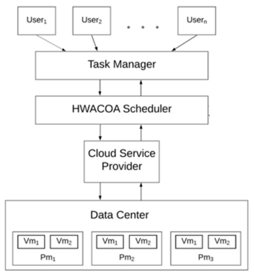
Figure 1. Architectural diagram of the task scheduler in cloud environment.

3.1. Task Scheduling Process Using HWACO Algorithm

The ACO (Ant Colony Optimization) algorithm, as the term suggests, tries to copy the behavior and movements of the ant toward a particular food source and back to its colony [19]. The algorithm comprises two major steps: the Construct_ANT solution and the Update_Pheromone function. In the Construct_ANT solution function, a set of artificial ants are constructed in order to find results from the finite set of available answer components, and, in the Update_Pheromone function, the pheromone level related to the solution set is maximized in order to arrive at an ideal solution-set from the available possible solution sets, that is, by maximizing the pheromone level related to a particular solution set, more importance is given to that particular solution set compared to other solution sets; therefore, selection of the ideal solution set occurs. Efficient discovery of the shortest path is important. At the same time, optimization is also one of the most vital factors in order to obtain and enhance the functioning of the task scheduler in the cloud environment. The Ant Colony Optimization algorithm and some other similar type of algorithms provide a near ideal solution with some drawbacks in certain cases; thus, an enhanced version of the ACO has been introduced, that is, the HWACO algorithm. The HWACO is equipped with improved construct ANT solution and Update Pheromone methods that make use of the weight concept, which provides the required consistency among the capabilities, such as exploitation and exploration. In this work, the HWACO algorithm was defined and executed in the task scheduling process using the following notation:

• S is the exploration space with a finite set of distinct choice variables generated for each variable Ti;
• Ω represents the set of restraints;
• f:S→R is the main function which must be reduced.

The definition of the exploration space $S$ is as follows. A distinct variable set $X_i$, where the value of i ranges from [1, m] (where m is the number of available tasks) with the variable’s value present in the set, is defined as $v_{ij}\in D_i$, and $D_i=⟨v1j,\dots , v_{\left|D_i\right|j}⟩$, where i represents a particular selected variable in the set $S$, and $D_i$ stands for the search variable for finding the correct virtual machine; therefore, $X_i$ represents the set of the available virtual machine for executing the required tasks. Each element of the set $S$ is defined properly, that is, every element variable $X_i$ has a value $v_{ij}$ allocated from its field $S$. A new set $S\Omega$ is defined, which contains the achievable results that satisfy all the constraints specified on the set $\Omega$ and set $X_i$. The constraints present in the set$\Omega$ are usually pre-fed beforehand to include various rules and constraints, such as checking the value of the elements from the different sets such as $S, T \mathrm{and} V,$ in order to make sure that these values are inside the acceptable range of values, and no negative numbers are present. The rule for forming various sets such as $X_i, D_i$, and others will eventually lead to finding the required objective solution set by setting up the fitness function and the selection of values based on the fitness function, and certain rules, such the maximum number of the available virtual machines to be considered, that is, the j value, the acceptable range of values for the constants such as $\alpha$, $\beta$, and many more depend on the user’s needs.

A result set S* that belongs to the set S_Ω is known as a global optimal solution set if it satisfies the below equation:

$$f\left(S^{\ast }\right)\le f\left(S\Omega \right) , \forall S\Omega \in S$$

(4)

In order to obtain the best optimal path with the shortest distance, the following processes are followed:

o

Construct_ANT solution.

o

Update_Pheromone.

3.2. Construct ANT Solution Process

A group of m artificial ants try to create the solution set by combining elements from the available finite set of existing solution mechanisms $S$, and the new set $C$, which is a subset of $X_i$ union $\Omega$ (here set $C$ and $S\Omega$ are the same), which is represented by the set $C\to \left[c_{ij}\right]$, where j = 1, …, |$D_i$| and i = 1, …, m. For an appropriate optimization process, the function begins with a null partial result, which is represented by $S^p=\varnothing$. After this, all of the present partial solution $S^p$ is then protracted at every construction step-by-step by adding a feasible solution component from the set of feasible neighbours $N(S^p) \subseteq C$, that is, in order to get to the solution component, the set of feasible neighbours $N(S^p)$ is used, and this set is calculated from the previously calculated solution component $S^p$, where the values of the ith task and the selected jth virtual machine are left, and, for assigning the (i+1)th task, the range of virtual machines to look for will be designed in such a way that it gives less priority to the already assigned virtual machines and gives more priority to the available virtual machines. The process of developing solutions can be thought of as a path on the construction graph $GC\left(V,E\right)$. The solution construction mechanism, which defines the set $N(S^p)$with respect to a partial solution $S^p$, implicitly defines the allowed paths in the $GC$. At each construction step, a remedy element from $N(S^p)$is chosen probabilistically. Thus, for assigning one task to the correct virtual machine, multiple comparison will be done based on the range of virtual machines, when the value of the element $c_{ij}$ obtained (ith task assigned to the jth virtual machine) matches with other elements from the $S^p$ set, that is, $c_{ij}=c_{il}$ and so on. Then, the Equation (5a) is used to calculate the best possible pair, but when the set has different values, Equation (5b) is used to calculate the best possible pair by using the weight concept. The main reason to use weights in the second case is because, when the value of the elements in set is different, this formula helps to determine the best pair of the task-to-virtual machine match, but, most of the time, it just acts like a cross-checker to be sure that the selection is optimal, and the selection eventually results in the required solution set that is optimal. The calculation of weights is done based on the first and second best values of the elements from the $S^p$ set, where $c_{ij}$ refers to the first highest value, and $c_{il}$ refers to the second highest value. The precise rules for the stochastic selection of solution components differ based on the cases mentioned below.

Case 1—when $c_{ij}=c_{il}$

$$p\left(\left.c_{i\left.j\right|k}\right|S^p\right)=\frac{T_{\mathrm{i}j}^{\alpha }\ast {\eta }_{\mathrm{i}j}^{\beta }}{{{\displaystyle \sum }}_{C_{il}\in N\left(s^p\right)}\left(T_{il}^{\alpha }\right)\ast \left({\eta }_{\mathrm{i}l}^{\beta }\right)}\forall c_{ij}{c}_{il}\in N\left(S^{\rho }\right)$$

(5a)

Case 2—when $c_{ij}\ne c_{il}$

$$p\left(\left.c_{i\left.j\right|k}\right|S^p\right)=\max \left[\left(\frac{T_{\mathrm{i}j}^{\alpha }\ast {\eta }_{\mathrm{i}j}^{\beta }}{{{\displaystyle \sum }}_{C_{il}\in N\left(s^p\right)}\left(T_{il}^{\alpha }\right)\ast \left({\eta }_{\mathrm{i}l}^{\beta }\right)}\ast w1\right) ,\left(\frac{T_{\mathrm{i}j}^{\alpha }\ast {\eta }_{\mathrm{i}j}^{\beta }}{{{\displaystyle \sum }}_{C_{il}\in N\left(s^p\right)}\left(T_{il}^{\alpha }\right)\ast \left({\eta }_{\mathrm{i}l}^{\beta }\right)}\ast \left(1-w1\right)\right)\right]\forall c_{ij}{c}_{il}\in N\left(S^{\rho }\right)$$

(5b)

The weights are calculated using the below-mentioned formula:

$$w1=\frac{p(j|l)\ast {\eta }_{ij}}{p(j|l)\ast {\eta }_{ij}+p(l|j)\ast {\eta }_{il}}$$

(5c)

where the current ith task can be assigned to a virtual machine from the range [j, k]. Here, the value of j initially starts from one, and, as the number of iterations increases, the value of j also increases, and the value of k is equivalent to the value of $D_i$ for that particular task; thus, $p\left(\left.c_{i\left.j\right|k}\right|S^p\right)$ represents the probabilistic value of selecting each virtual machine from the above range for processing the ith task. Variables, ${\eta }_{ij}$ and ${\tau }_{ij}$ are correspondingly the heuristic value and pheromone value, respectively, connected with the component $c_{ij}$. The variable ${\eta }_{ij}$ is a constant value for any value of i, j, which is fixed beforehand, and the variable ${\tau }_{ij}$ is calculated using the Update_Pheromone update function. The constant variables such as $\alpha$ and $\beta$ are the makespan and cost constant variables, respectively, whose values are similar to the makespan and cost constants values used in the objective function in Equation (1).

3.3. Update_Pheromone Process

The pheromones update step aims to maximizes the pheromone values related to the result set while decreasing those related with corrupt result sets. Typically, this is accomplished by (i) reducing all pheromone values via evaporation of the pheromones and (ii) maximizing the levels of pheromones related with a selected set of good results S*:

$$\tau ij=\left(1-p\right)\tau ij+\mathrm{\Delta }{T}_{ij}^{\ast }$$

(6a)

$$\mathrm{\Delta }{T}_{ij}^{\ast }=p\cdot {\displaystyle \sum }_{sϵSupd | cij ϵ S }F\left(s\right)$$

(6b)

where S* represents the solution set that is used in the updating process, and p is based on the previously calculated value of the term $p\left(\left.c_{i\left.j\right|k}\right|S^p\right)$. This constraint is called the evaporation rate. F is defined as the function of the the equation that follows:

$$f\left(s\right)<f\left(s^{\prime }\right)=>F\left(s\right)\ge F\left(s^{\prime }\right), \forall s\ne s^{\prime }\in S$$

(7)

Here, $f\left(s\right)$ represents the fitness function of an element (s) from the set such that, when compared with other elements (suppose s’), the fitness function of $f\left(s\right)$ is low compared to other elements present in the set, and, at the same time, the $F\left(s\right)$ value should be high. Here, $F\left(s\right)$ stands for the performance in of that element in comparison to other elements in the set. The performance test will be calculated based on the fitness function $f\left(s\right)$ and $f\left(s^{\prime }\right)$, and the average mean to get the performance in terms of percentage value and this value should be higher. The reason to select the average mean method is because this formula will be used multiple times, and conducting a dedicated parameterized test, such as a t-test, will increase the makespan of the algorithm. Thus, a simple test is selected to measure the performance metrics of the selected task-to-virtual machine pairs and obtain an optimal solution set.

Pheromone evaporation is a beneficial way of overlooking that encourages the search for new ranges in the exploration space. Various ACO programs and methods, such as the Ant Colony System (ACS), Ant Colony Optimization (ACO), and many others try to increase the performance of the cloud environment by using this method, but they have certain drawbacks, due to which the objective of improving the performance is not seen in such algorithms, yet the performance of the introduced HWACO algorithm is theoretically high, due to the concept of weight and other functionalities used in the algorithm. Current knowledge, including substantive findings of the above-mentioned update rule, are obtained through various conditions of the S_upd, which is often considered a subset of S_iter ∪ {S_bs}, where S_iter is the solution set constructed in the current iteration, and S_bs is the best-so-far solution, that is, the best answer discovered since the first algorithm iteration is another mechanism that boosts the performance of the introduced algorithm.

$$S*\leftarrow Siter U Sbs$$

(8)

3.4. Algorithm

From the below HWACO Algorithm 1, it is clear that the introduced algorithm makes use of weight, and this is reflected in Equations (5a) and (5b) based on the conditions, whereas the normal ACO algorithm will use just one equation that is similar to Equation (5a). Thus, the search space will be more compared to the HWACO, and the updating process is more static in nature, as it assumes the p evaporation rate to be constant, thus making the process more static in nature. In contrast, in the HWACO, the evaporation rate is determined based on the past values, thus making it more dynamic in nature. Therefore, all the formulas and explanation point to the fact that the introduced algorithm is better compared to the ACO algorithm.

Algorithm 1: HWACO Scheduler.

Input: Inputs considered: Number of tasks—$T_1, T_2, \dots , T_m$ (m refers to number of tasks) Number of virtual machines—$v_1, v_2, \dots , v_n$ (n refers to number of virtual machine) Maximum iteration—$Ma{x}^t$ Number of host machines—$k$ Output: Mapping (Ti -> Vj) for all the available tasks for the set of virtual machines, which may be present in the same host machine or distributed over multiple virtual machines. Proposed HWACO Scheduler: BEGIN Initialize the population and number of generations of ants and other parameters WHILE t < Maxt Compute the path of the ant by Equation (5); Perform the Update_Pheromone update process by using Equation (6); IF (The fitness function is evaluated using the Equation (7)) Evaluate the best solution of that iteration using Equations (2) and (3); Compute the objective function using Equation (1); IF (objective_function_value < S* check the condition in Equation (4)) update S* using Equation (8) END IF END IF Increment the value of t by 1; END WHILE Return the S*, which contains the best solution END

4. Results and Discussion

All the finds and experiments were conducted in a simulated environment with initial setup details mentioned in Table 2 and Table 3 using the Java (JDK 1.6)-based Cloudsim tool. All the experiments were conducted by varying the task inputs from 100–400 units [20,24]. The performance of the introduced Hybrid Weighted Ant Colony Optimized algorithm was compared with various other algorithms, such as the MTF-BPSO [14],QANA [25], ACO [28], MIN-MIN [29], FCFS [30], with respect to their time taken for execution (makespan) and cost parameters. The main reason to select the ACO algorithm is due to the fact that the introduced algorithm is based on ACO, and, thus, the first algorithm used for comparison was the ACO algorithm, while the other algorithm used for comparison could have been any recently proposed or a traditional one, but out of all the algorithms, FCFS and MIN-MIN were selected due to various reasons. Both of them are the most basic and traditional algorithms which were initially utilized in almost all cloud computing and the fact that most of the algorithms that we know of today are related to these algorithms in some or the other way. These were mainly the task scheduling algorithms which consider makespan and cost as their parameters for evaluation of their performance. Thus, these two algorithms acted as a stepping stone to decide whether the introduced algorithm would be able to optimize the result and achieve the objective goals. The selection for QANA is based on the fact that QANA is one of the state-of-the-art algorithms introduced for solving global optimization problems, that is, QANA is better in terms of performances for returning ideal optimization solutions when compared to other modern algorithms like the MWOA (Modified Whale Optimization Algorithm), EEGWO (Exploration-Enhanced Grey Wolf Optimizer), and many more. Thus, the introduced algorithm was compared with ideal algorithms, such as FCFS and MIN-MIN. At the same time, it was also compared with modern algorithms such as QANA and MTF-BPSO in terms of performance. Finally, MTF-BPSO was selected because MTF-BPSO is one of the recently proposed algorithms which aims to improve the performance task scheduling and quality of service in cloud computing and for the fact that MTF-BPSO outperforms many task scheduling algorithms such as the Sailfish Optimization Algorithm, Opposition-Based Sunflower Optimization Algorithm, and many other algorithms.

There were numerous parameters utilized for the input, which are as follows:

Table 2. Simulation setup.

S/No	Entity Type	Parameter	Value
1	User	Number of users	50
2	Task	Size	400
		Number of tasks	100–400
3	Host	Host memory (RAM)	2048BM
		Host bandwidth	10,000
		Host storage	100,000
4	Virtual Machine (VM)	Type of policy	Time-Shared
		Number of VMs	40
		VM RAM	512BM
		VMM	Xen
		OS	Windows
		Number of CPUs	1 on each
5	Datacentre	Number of datasets	4
		Number of hosts	2

Table 2. Simulation setup.

S/No	Entity Type	Parameter	Value
1	User	Number of users	50
2	Task	Size	400
		Number of tasks	100–400
3	Host	Host memory (RAM)	2048BM
		Host bandwidth	10,000
		Host storage	100,000
4	Virtual Machine (VM)	Type of policy	Time-Shared
		Number of VMs	40
		VM RAM	512BM
		VMM	Xen
		OS	Windows
		Number of CPUs	1 on each
5	Datacentre	Number of datasets	4
		Number of hosts	2

The values used for initializing the parameters and hyperparameters in all the six algorithms are present in Table 3 and Table 4. Parameters are generally values which are calculated during the process of finding the solution set, that is, they are variables that help determine the final optimal solution set. On the other hand, hyperparameters are fixed values which help determine the parametric values during each iteration.

Table 3. Parameter initialization.

S/No.	Scheduling Algorithms	Parameters	Values
1	HWACO	Number of ants in colony	1000
		Makespan constant (α)	0.3
		Cost constant (β)	0.6
		Heuristic constant (n)	0.498
2	ACO	Number of ants in colony	1000
		Evaporation factor (p)	0.398
		Pheromone tracking weight (α)	0.3
		Heuristic information weight (β)	0.6
		Pheromone updating constant (q)	10
3	MIN-MIN	Makespan constant (α)	0.3
		Cost constant (β)	0.6
		Population size	1000
4	FCFS	Makespan constant (α)	0.3
		Cost constant (β)	0.6
		Population size	1000
5	QANA	The number of flocks (k)	10
		Memory size (K’)	8
		Short-term memory with memory size (Ҡ”)	48
6	MTF-BPSO	Decision variable £	1 or 0 depending on task size
		Social learning factor c1	0.5
		Personal learning factor c2	2.4
		Inertia factor	0.7

Table 3. Parameter initialization.

S/No.	Scheduling Algorithms	Parameters	Values
1	HWACO	Number of ants in colony	1000
		Makespan constant (α)	0.3
		Cost constant (β)	0.6
		Heuristic constant (n)	0.498
2	ACO	Number of ants in colony	1000
		Evaporation factor (p)	0.398
		Pheromone tracking weight (α)	0.3
		Heuristic information weight (β)	0.6
		Pheromone updating constant (q)	10
3	MIN-MIN	Makespan constant (α)	0.3
		Cost constant (β)	0.6
		Population size	1000
4	FCFS	Makespan constant (α)	0.3
		Cost constant (β)	0.6
		Population size	1000
5	QANA	The number of flocks (k)	10
		Memory size (K’)	8
		Short-term memory with memory size (Ҡ”)	48
6	MTF-BPSO	Decision variable £	1 or 0 depending on task size
		Social learning factor c1	0.5
		Personal learning factor c2	2.4
		Inertia factor	0.7

4.1. Makespan Valuation

In this unit, the performance of the presented algorithm in terms of the time taken for the execution of the task was assessed. To evaluate performance, 100 to 400 tasks were considered, and these tasks were executed with onset rates ranging between 10 and 40. Here the onset rate represents the time duration (in microseconds) after which each task is given to the algorithm, that is, the algorithm will become overwhelmed with handling a large number of tasks when assigned immediately. Thus, to prevent this from happening and maintain a low bandwidth in the communication bus, the onset rate was used with different values. The results of the proposed method were compared among those of the HWACO, QANA, MTF-BPSO, ACO, MIN-MIN, and FCFS. Figure 1 and Figure 2 show the results of the simulation.

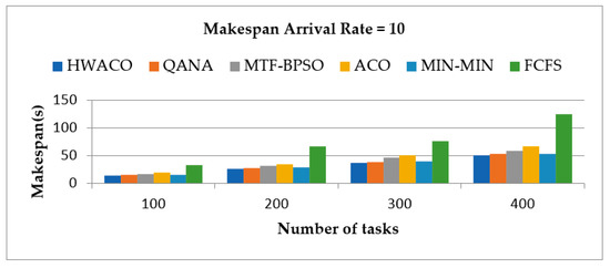
Figure 2. Execution time for the tasks with onset rate of 10.

4.1.1. Makespan, Onset Rate = 10

In this unit, we measured the time taken to execute the tasks with 10 as the onset rate. The time taken for time, in microseconds, for various algorithms such as HWACO, QANA, MTF-BPSO, ACO, MIN-MIN and FCFS was 13.78, 15.01, 16.21, 18.8, 15.73, and 32.32, respectively. When the number of tasks was changed to 200, the time taken for the execution for the HWACO, QANA, MTF-BPSO, ACO, MIN-MIN, and FCFS was 25.9, 27.23, 31.09, 34.61, 29.05, and 67, respectively. When the number of tasks was changed to 300, the time taken for the execution for HWACO, QANA, MTF-BPSO, ACO, MIN-MIN, and FCFS was 36.56, 38.31, 46.31, 50.31, 40.02, and 75.5, respectively. Finally, when the number of tasks was changed to 400, the time taken for the execution for HWACO, QANA, MTF-BPSO, ACO, MIN-MIN, and FCFS was 50.4, 52.3, 58.42, 66, 53.1, and 124, respectively. Figure 2 shows the execution time for the tasks by different algorithms when the onset rate = 10.

4.1.2. Makespan, Onset Rate = 40

In this unit, we considered the time taken to execute the tasks with 40 as the onset rate. The time taken for execution for HWACO, QANA, MTF-BPSO, ACO, MIN-MIN, and FCFS was 16.98, 17.01, 19.67, 22.68, 18.786, and 38.784, respectively. When the number of tasks was increased to 200, the time taken for the execution for HWACO, QANA, MTF-BPSO, ACO, MIN-MIN, and FCFS was 30.76, 32.36, 38.12, 41.53, 34.86, and 80.4, respectively. When the number of tasks was changed to 300, the time taken for the execution for HWACO, QANA, MTF-BPSO, ACO, MIN-MIN, and FCFS was 45.13, 46.12, 55.41, 60.37, 48.02, and 90.6, respectively. Finally, when the number of tasks was changed to 400, the time taken for the execution for HWACO, QANA, MTF-BPSO, ACO, MIN-MIN, and FCFS was 60.8, 62.3, 71.01, 79.2, 63.98, and 148.8, respectively. Figure 3 shows the execution time for the tasks by different algorithms when the onset rate = 40.

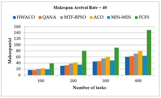
Figure 3. Execution time for the tasks with onset rate of 40.

Figure 4 shows the convergence plot when the makespan of 200 tasks was considered. The results of the proposed method were compared among the HWACO, QANA, MTF-BPSO, ACO, MIN-MIN, and FCFS.

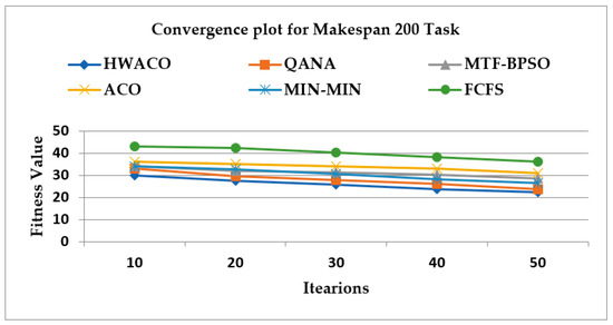
Figure 4. The convergence plot for makespan of 200 tasks.

Figure 5 shows the convergence plot when the makespan of 400 tasks was considered. The results of the proposed method were compared among the HWACO, QANA, MTF-BPSO, ACO, MIN-MIN, and FCFS.

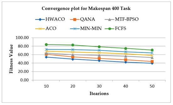
Figure 5. The convergence plot for makespan of 400 tasks.

4.2. Cost Assessment

The cost assessment was evaluated in this section. In this virtual simulation process, 200 and 400 tasks with varying deadlines were considered. The iteration was between 10 to 50. Figure 6 and Figure 7 show the results that were obtained. Figure 6 considers 200 task cost values, while Figure 7 considers 400 task cost values. Cost assessment of the proposed algorithm HWACO was compared with other algorithms, including QANA, MTF-BPSO, ACO, MIN-MIN, and FCFS. From the experimental results obtained, they suggest that the introduced algorithm HWACO achieved a low cost for both cases when number of tasks were 200 and 400.

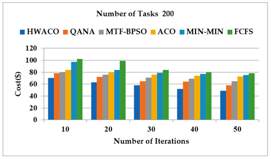
Figure 6. The task cost values of 200.

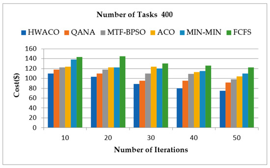
Figure 7. The task cost values of 400.

4.3. Statistical Analysis Using t-Test

Table 4, Table 5, Table 6, Table 7, Table 8, Table 9, Table 10, Table 11, Table 12 and Table 13 contain the outcomes of a paired t-test that was carried out to assess whether there are substantial changes between the makespan and cost obtained from the proposed algorithm—HWACO—and other algorithms, namely, QANA, MTF-BPSO, ACO, MIN-MIN, and FCFS, using comparable stopping standards for all task instances. The satisfactory p-value must be less than alpha α < 0.5. As shown in the tables below, almost all of the datasets had p-values that were less than this alpha value, which shows a substantial enhancement in the proposed HWACO algorithm compared to the other algorithms used for comparison. Thus, it can be inferred that the HWACO outperforms other task scheduling algorithm in terms of makespan and cost.

Table 4. t-Test for makespan between HWACO and QANA.

Makespan	Task Size	HWACO	QANA	Improvement	t-Test Value	p-Value
Onset rate 10	100	13.78	15.01	8.194536975	3.4534	7.430 × 10−3
	200	25.9	27.23	4.884318766	2.4533	4.405 × 10−2
	300	36.56	38.31	4.567997912	3.3093	6.351 × 10−2
	400	50.4	52.3	3.632887189	2.4534	9.984 × 10−2
Onset rate 40	100	16.98	17.01	0.176366843	1.9093	1.308 × 10−2
	200	30.76	32.26	4.649721017	2.4532	4.304 × 10−4
	300	45.13	46.12	2.146574154	2.0984	6.094 × 10−2
	400	60.8	62.3	2.407704655	2.3221	5.534 × 10−3

Table 4. t-Test for makespan between HWACO and QANA.

Makespan	Task Size	HWACO	QANA	Improvement	t-Test Value	p-Value
Onset rate 10	100	13.78	15.01	8.194536975	3.4534	7.430 × 10−3
	200	25.9	27.23	4.884318766	2.4533	4.405 × 10−2
	300	36.56	38.31	4.567997912	3.3093	6.351 × 10−2
	400	50.4	52.3	3.632887189	2.4534	9.984 × 10−2
Onset rate 40	100	16.98	17.01	0.176366843	1.9093	1.308 × 10−2
	200	30.76	32.26	4.649721017	2.4532	4.304 × 10−4
	300	45.13	46.12	2.146574154	2.0984	6.094 × 10−2
	400	60.8	62.3	2.407704655	2.3221	5.534 × 10−3

Table 5. t-Test for makespan between HWACO and MFT-BPSO.

Makespan	Task Size	HWACO	MFT-BPSO	Improvement	t-Test Value	p-Value
Onset rate 10	100	13.78	16.21	14.99074645	2.3498	5.394 × 10−3
	200	25.9	31.09	16.69347057	2.4085	6.048 × 10−4
	300	36.56	46.31	21.05376808	3.2083	3.308 × 10−5
	400	50.4	58.42	13.72817528	2.1083	8.073 × 10−3
Onset rate 40	100	16.98	19.67	13.6756482	2.8992	1.937 × 10−3
	200	30.76	38.12	19.30745016	3.4913	4.497 × 10−4
	300	45.13	55.41	18.55260783	2.8934	1.003 × 10−4
	400	60.8	71.01	14.37825658	2.5085	4.999 × 10−3

Table 6. t-Test for makespan between HWACO and ACO.

Makespan	Task Size	HWACO	ACO	Improvement	t-Test Value	p-Value
Onset rate 10	100	13.78	18.9	27.08994709	5.4535	5.563 × 10−4
	200	25.9	34.61	25.16613695	5.2434	8.456 × 10−3
	300	36.56	50.31	27.33055059	4.9305	2.344 × 10−4
	400	50.4	66	23.63636364	5.8497	1.084 × 10−2
Onset rate 40	100	16.98	22.68	25.13227513	4.2433	9.083 × 10−3
	200	30.76	41.53	25.93306044	4.9085	4.304 × 10−5
	300	45.13	60.37	25.24432665	5.2324	7.305 × 10−4
	400	60.8	79.2	23.23232323	3.5345	3.405 × 10−3

Table 7. t-Test for makespan between HWACO and MIN-MIN.

Makespan	Task Size	HWACO	MIN-MIN	Improvement	t-Test Value	p-Value
Onset rate 10	100	13.78	15.73	12.39669421	3.5673	6.451 × 10−3
	200	25.9	29.05	10.84337349	3.2324	4.454 × 10−3
	300	36.56	40.02	8.645677161	2.9038	3.408 × 10−2
	400	50.4	53.1	5.084745763	3.0485	2.532 × 10−2
Onset rate 40	100	16.98	18.786	9.613541999	3.8058	5.403 × 10−3
	200	30.76	34.86	11.76133104	4.0835	6.358 × 10−3
	300	45.13	48.02	6.018325698	2.0805	4.456 × 10−2
	400	60.8	63.98	4.97030322	4.3034	9.308 × 10−2

Table 8. t-Test for makespan between HWACO and FCFS.

Makespan	Task Size	HWACO	FCFS	Improvement	t-Test Value	p-Value
Onset rate 10	100	13.78	32.32	57.36386139	4.3533	8.354 × 10−5
	200	25.9	67	61.34328358	3.0835	6.038 × 10−7
	300	36.56	75.5	51.57615894	4.5089	6.305 × 10−5
	400	50.4	124	59.35483871	5.3508	9.312 × 10−6
Onset rate 40	100	16.98	38.784	56.21905941	4.9248	8.038 × 10−5
	200	30.76	80.4	61.74129353	3.3083	9.352 × 10−7
	300	45.13	90.6	50.18763797	4.1244	6.353 × 10−5
	400	60.8	148.8	59.13978495	5.0493	5.354 × 10−6

Table 9. t-Test for cost between HWACO and QANA.

Cost	Iteration	HWACO	QANA	Improvement	t-Test Value	p-Value
Number of Task 200	10	70	78	10.25641026	4.3534	5.342 × 10−2
	20	63	72	12.5	5.3503	6.405 × 10−2
	30	58	65	10.76923077	3.4533	3.035 × 10−2
	40	52	64	18.75	4.3422	8.308 × 10−3
	50	49	58	15.51724138	3.4508	7.083 × 10−3
Number of Task 400	10	110	118	6.779661017	5.3058	9.304 × 10−2
	20	103	110	6.363636364	3.3058	5.204 × 10−2
	30	89	95	6.315789474	4.2398	3.038 × 10−2
	40	80	95	15.78947368	3.0583	5.035 × 10−3
	50	75	92	18.47826087	4.3583	9.083 × 10−3

Table 10. t-Test for cost between HWACO and MTF-BPSO.

Cost	Iteration	HWACO	MTF-BPSO	Improvement	t-Test Value	p-Value
Number of Task 200	10	70	80	12.5	4.0834	5.038 × 10−2
	20	63	76	17.10526316	3.3508	6.043 × 10−3
	30	58	71	18.30985915	3.9553	1.301 × 10−3
	40	52	69	24.63768116	4.2316	9.085 × 10−4
	50	49	65	24.61538462	3.9358	7.032 × 10−4
Number of Task 400	10	110	122	9.836065574	3.1239	5.034 × 10−2
	20	103	118	12.71186441	3.9835	8.342 × 10−2
	30	89	110	19.09090909	4.0023	4.497 × 10−3
	40	80	109	26.60550459	3.8947	1.242 × 10−4
	50	75	98	23.46938776	5.2948	5.099 × 10−4

Table 11. t-Test for cost between HWACO and ACO.

Cost	Iteration	HWACO	ACO	Improvement	t-Test Value	p-Value
Number of Task 200	10	70	84	16.66666667	3.3048	4.534 × 10−3
	20	63	80	21.25	2.5034	3.395 × 10−4
	30	58	76	23.68421053	3.0485	8.035 × 10−4
	40	52	74	29.72972973	3.9853	7.357 × 10−4
	50	49	73	32.87671233	3.4532	4.048 × 10−4
Number of Task 400	10	110	124	11.29032258	2.3934	9.825 × 10−2
	20	103	122	15.57377049	3.0385	4.397 × 10−3
	30	89	124	28.22580645	4.2311	7.092 × 10−4
	40	80	113	29.20353982	4.3244	2.139 × 10−4
	50	75	104	27.88461538	4.1333	1.082 × 10−4

Table 12. t-Test for cost between HWACO and MIN-MIN.

Cost	Iteration	HWACO	MIN-MIN	Improvement	t-Test Value	p-Value
Number of Task 200	10	70	97	27.83505155	4.5654	4.455 × 10−4
	20	63	84	25	5.4213	6.048 × 10−4
	30	58	79	26.58227848	4.2324	4.484 × 10−4
	40	52	77	32.46753247	5.2342	2.304 × 10−5
	50	49	75	34.66666667	4.3297	1.398 × 10−5
Number of Task 400	10	110	138	20.28985507	3.2497	9.038 × 10−3
	20	103	122	15.57377049	2.2491	5.038 × 10−3
	30	89	120	25.83333333	2.3423	3.395 × 10−3
	40	80	115	30.43478261	3.0382	7.458 × 10−4
	50	75	110	31.81818182	4.3948	9.344 × 10−4

Table 13. t-Test for cost between HWACO and FCFS.

Cost	Iteration	HWACO	FCFS	Improvement	t-Test Value	p-Value
Number of Task 200	10	70	102	31.37254902	4.3422	5.056 × 10−4
	20	63	99	36.36363636	3.3508	7.058 × 10−5
	30	58	84	30.95238095	3.2443	9.956 × 10−4
	40	52	80	35	2.9457	8.947 × 10−5
	50	49	78	37.17948718	4.2498	3.305 × 10−5
Number of Task 400	10	110	143	23.07692308	3.9375	1.084 × 10−4
	20	103	145	28.96551724	2.0948	2.009 × 10−4
	30	89	130	31.53846154	3.0358	5.045 × 10−4
	40	80	126	36.50793651	2.3957	6.084 × 10−5
	50	75	122	38.52459016	3.0358	9.083 × 10−6

5. Conclusions

Given that the scheduling of the task process is one of the most vital issues encountered by the cloud environment, this paper proposed a new algorithm called the HWACO algorithm that improves the basic functions of the ACO algorithm in order to efficiently search through the solution space and return the best optimal solution. This was achieved by using two main functions, which are the Construct_ANT solution function and Update_Pheromone function, respectively, that try to find the best and optimal solution, as was mentioned in Section 3. As mentioned earlier, the selection of the best solution is based on the values computed using the objective formula which combines both the makespan and cost parameters. Thus, the proposed algorithm outperformed other algorithms in terms of cost and makespan in such a way that the makespan and cost of the entire process were minimized, and, at the same time, the performance of the cloud computing environment was increased. To support this claim, an experimental simulation was conducted along with the statistical t-test, which suggest the fact that the HWACO was able to attain an average of 3.83%, 16.54%, 25.34%, 8.66% and 57.11% of improvement when compared to the QANA, MTF-BPSO, ACO, MIN-MIN, and FCFS in terms of makespan, respectively, and 12.15%, 18.88%, 23.63%, 27.05% and 32.94% of improvement when compared to QANA, MTF-BPSO, ACO, MIN-MIN, and FCFS, respectively, in terms of cost. Therefore, it can be concluded that the introduced algorithm optimizes the performance of the task scheduler in terms of makespan and cost.

References

- Zuo, X.; Zhang, G.; Tan, W. Self-Adaptive Learning PSO-Based Deadline Constrained Task Scheduling for Hybrid IaaS Cloud. IEEE Trans. Autom. Sci. Eng. 2013, 11, 564–573. [Google Scholar] [CrossRef]
- Krishnadoss, P.; Pradeep, N.; Ali, J.; Nanjappan, M.; Krishnamoorthy, P.; Kedalu Poornachary, V. CCSA: Hybrid cuckoo crow search algorithm for task scheduling in cloud computing. Int. J. Intell. Eng. Syst. 2021, 14, 241–250. [Google Scholar] [CrossRef]
- Pradeep, K.; Jacob, T.P. CGSA scheduler: A multi-objective-based hybrid approach for task scheduling in cloud environment. Inf. Secur. J. 2018, 27, 77–91. [Google Scholar] [CrossRef]
- Pradeep, K.; Ali, L.J.; Gobalakrishnan, N.; Raman, C.J.; Manikandan, N. CWOA: Hybrid Approach for Task Scheduling in Cloud Environment. Comput. J. 2021, 65, 1860–1873. [Google Scholar] [CrossRef]
- Krishnadoss, P.; Chandrashekar, C.; Poornachary, V.K. RCOA Scheduler: Rider Cuckoo Optimization Algorithm for Task Scheduling in Cloud Computing. Int. J. Intell. Eng. Syst. 2022, 15, 1–10. [Google Scholar]
- Nabi, S.; Aleem, M.; Ahmed, M.; Islam, M.A.; Iqbal, M.A. RADL: A resource and deadline-aware dynamic load-balancer for cloud tasks. J. Supercomput. 2022, 78, 14231–14265. [Google Scholar] [CrossRef]
- Konjaang, J.K.; Murphy, J.; Murphy, L. Energy-efficient virtual-machine mapping algorithm (EViMA) for workflow tasks with deadlines in a cloud environment. J. Netw. Comput. Appl. 2022, 203, 103400. [Google Scholar] [CrossRef]
- Kumar, M.; Suman, S. Scheduling in IaaS Cloud Computing Environment using Sailfish Optimization Algorithm. Trends Sci. 2022, 19, 4204. [Google Scholar] [CrossRef]
- Gupta, S.; Singh, R.S.; Vasant, U.D.; Saxena, V. User defined weight based budget and deadline constrained workflow scheduling in cloud. Concurr. Comput. Pract. Exp. 2021, 33, e6454. [Google Scholar] [CrossRef]
- Bacanin, N.; Zivkovic, M.; Bezdan, T.; Venkatachalam, K.; Abouhawwash, M. Modified firefly algorithm for workflow scheduling in cloud-edge environment. Neural Comput. Appl. 2022, 34, 9043–9068. [Google Scholar] [CrossRef]
- Chandrashekar, C.; Krishnadoss, P. Opposition based sunflower optimization algorithm using cloud computing environments. Mater. Today Proc. 2022, 62, 4896–4902. [Google Scholar] [CrossRef]
- Gokuldhev, M.; Singaravel, G. Local Pollination-Based Moth Search Algorithm for Task-Scheduling Heterogeneous Cloud Environment. Comput. J. 2022, 65, 382–395. [Google Scholar] [CrossRef]
- Belgacem, A.; Beghdad-Bey, K.; Nacer, H.; Bouznad, S. Efficient dynamic resource allocation method for cloud computing environment. Clust. Comput. 2020, 23, 2871–2889. [Google Scholar] [CrossRef]
- Kumar, M.; Sharma, S.C.; Goel, S.; Mishra, S.K.; Husain, A. Autonomic cloud resource provisioning and scheduling using meta-heuristic algorithm. Neural Comput. Appl. 2020, 32, 18285–18303. [Google Scholar] [CrossRef]
- Nanjappan, M.; Natesan, G.; Krishnadoss, P. An Adaptive Neuro-Fuzzy Inference System and Black Widow Optimization Approach for Optimal Resource Utilization and Task Scheduling in a Cloud Environment. Wirel. Pers. Commun. 2021, 121, 1891–1916. [Google Scholar] [CrossRef]
- Nadimi-Shahraki, M.H.; Zamani, H. DMDE: Diversity-maintained multi-trial vector differential evolution algorithm for non-decomposition large-scale global optimization. Expert Syst. Appl. 2022, 198, 116895. [Google Scholar] [CrossRef]
- Nadimi-Shahraki, M.H.; Zamani, H.; Mirjalili, S. Enhanced whale optimization algorithm for medical feature selection: A COVID-19 case study. Comput. Biol. Med. 2022, 148, 105858. [Google Scholar] [CrossRef]
- Zamani, H.; Nadimi-Shahraki, M.H.; Gandomi, A.H. Starling murmuration optimizer: A novel bio-inspired algorithm for global and engineering optimization. Comput. Methods Appl. Mech. Eng. 2022, 392, 114616. [Google Scholar] [CrossRef]
- Zuo, L.; Shu, L.; Dong, S.; Zhu, C.; Hara, T. A multi-objective optimization scheduling method based on the ant colony algorithm in cloud computing. IEEE Access 2015, 3, 2687–2699. [Google Scholar] [CrossRef]
- Batista, B.G.; Estrella, J.C.; Ferreira, C.H.G.; Filho, D.M.L.; Nakamura, L.H.V.; Reiff-Marganiec, S.; Santana, M.J.; Santana, R.H.C. Performance evaluation of resource management in cloud computing environments. PLoS ONE 2015, 10, e0141914. [Google Scholar] [CrossRef]
- Abdulhamid, S.I.M.; Abd Latiff, M.S.; Abdul-Salaam, G.; Hussain Madni, S.H. Secure scientific applications scheduling technique for cloud computing environment using global league championship algorithm. PLoS ONE 2016, 11, e0158102. [Google Scholar] [CrossRef] [PubMed]
- Abdullahi, M.; Ngadi, M.A. Symbiotic organism search optimization based task scheduling in cloud computing environment. Future Gener. Comput. Syst. 2016, 56, 640–650. [Google Scholar] [CrossRef]
- Ramezani, F.; Lu, J.; Hussain, F.K. Task-Based System Load Balancing in Cloud Computing Using Particle Swarm Optimization. Int. J. Parallel Program. 2014, 42, 739–754. [Google Scholar] [CrossRef]
- Domanal, S.G.; Guddeti, R.M.R.; Buyya, R. A Hybrid Bio-Inspired Algorithm for Scheduling and Resource Management in Cloud Environment. IEEE Trans. Serv. Comput. 2017, 13, 3–15. [Google Scholar] [CrossRef]
- Zamani, H.; Nadimi-Shahraki, M.H.; Gandomi, A.H. QANA: Quantum-based avian navigation optimizer algorithm. Eng. Appl. Artif. Intell. 2021, 104, 104314. [Google Scholar] [CrossRef]
- Sardaraz, M.; Tahir, M. A parallel multi-objective genetic algorithm for scheduling scientific workflows in cloud computing. Int. J. Distrib. Sens. Netw. 2020, 16, 1550147720949142. [Google Scholar] [CrossRef]
- Konjaang, J.K.; Xu, L. Multi-objective workflow optimization strategy (MOWOS) for cloud computing. J. Cloud Comput. 2021, 10, 11. [Google Scholar] [CrossRef]
- Yu, Q.; Ling, C.; Bin, L. Ant colony optimization applied to web service compositions in cloud computing. Comput. Electr. Eng. 2015, 41, 18–27. [Google Scholar] [CrossRef]
- Murad, S.S.; Badeel, R.O.Z.I.N.; Salih, N.; Alsandi, A.; Faraj, R.; Ahmed, A.R.; Alsandi, N. Optimized Min-Min task scheduling algorithm for scientific workflows in a cloud environment. J. Theor. Appl. Inf. Technol. 2022, 100, 480–506. [Google Scholar]
- Ramkumar, K.; Gunasekaran, G. Preserving security using crisscross AES and FCFS scheduling in cloud computing. Int. J. Adv. Intell. Paradig. 2019, 12, 77–85. [Google Scholar] [CrossRef]
Disclaimer/Publisher’s Note: The st atements, opinions and data contained in all publications are solely those of the individual author(s) and contributor(s) and not of MDPI and/or the editor(s). MDPI and/or the editor(s) disclaim responsibility for any injury to people or property resulting from any ideas, methods, instructions or products referred to in the content. |
Disclaimer/Publisher’s Note: The statements, opinions and data contained in all publications are solely those of the individual author(s) and contributor(s) and not of MDPI and/or the editor(s). MDPI and/or the editor(s) disclaim responsibility for any injury to people or property resulting from any ideas, methods, instructions or products referred to in the content. |
© 2023 by the authors. Licensee MDPI, Basel, Switzerland. This article is an open access article distributed under the terms and conditions of the Creative Commons Attribution (CC BY) license (https://creativecommons.org/licenses/by/4.0/).