Abstract
Detecting and tracking objects of interest in videos is a technology that can be used in various applications. For example, identifying cell movements or mutations through videos obtained in real time can be useful information for decision making in the medical field. However, depending on the situation, the quality of the video may be below the expected level, and in this case, it may be difficult to check necessary information. To overcome this problem, we proposed a technique to effectively track objects by modifying the simplest color balance (SCB) technique. An optimal object detection method was devised by mixing the modified SCB algorithm and a binarization technique. We presented a method of displaying object labels on a per-frame basis to track object movements in a video. Detecting objects and tagging labels through this method can be used to generate object motion-based prediction training data for machine learning. That is, based on the generated training data, it is possible to implement an artificial intelligence model for an expert system based on various object motion measurements. As a result, the main object detection accuracy in noisy videos was more than 95%. This method also reduced the tracking loss rate to less than 10%.
1. Introduction
Finding a specific object in an image can be used in many ways in our lives. This technology can be used to check whether restricted items are brought in when entering a specific place and can be used to check the presence of harmful objects. Under this circumstance, it can be said that identifying an object of interest in a video rather than a still image is a more important technique. Any information generated after identifying an important object in a video shot in real time can be used for making necessary decisions in the fields of security or medical care. However, it is difficult to track an object of interest in an environment in which the quality of a captured image is not sufficiently good, for example, in a microscopic medical field, a night security image, etc., due to image noise or ambiguity of the object.
To overcome this problem, we proposed a technique for tracking a moving object of interest in a noisy video. In general, various methods using machine learning have been proposed to track objects in images [1,2,3,4,5,6,7,8,9,10,11,12,13,14,15,16,17,18,19,20]. However, when the shape of the object to be tracked cannot be specified due to the low quality of the image, it is difficult to construct the training data. Because of this, it can be difficult to apply machine learning itself. To track an object without a separate data set in such an environment, we proposed an object detection and tracking algorithm based on the simplest color balance (SCB) technique [21]. The proposed method unifies the image information corresponding to the object to be detected through the SCB algorithm. The “information” refers to the pixel’s value in this paper. Then, the unified pixels and the remaining pixels are separated and binarized into the object of interest and the background, respectively. Finally, only the desired object is extracted from the binarized image.
The features of the SCB algorithm are as follows. The SCB specifies the upper and lower value ranges of pixels in the image. Thereafter, pixels within the corresponding range are collectively replaced with the minimum and maximum values of the available pixel values. For example, in the case of an 8-bit scale, 0 and 255 are designated, respectively. Afterwards, the histogram of pixel values that do not belong to the lower and upper ranges is stretched as much as possible within the given value scale and normalized to improve the quality, including the color balance of the image. In the task we need to process, the object of interest in the captured image is usually darker than the background. In addition, we did not consider the improvement of image quality when applying the SCB algorithm.
In this paper, we adopted the idea of collectively minimizing a certain low range of values in the SCB algorithm. In other words, we selected a value range that can be judged as an interested object among the dark pixels of the image. Then, SCB was applied to collectively substitute 0 for values smaller than the corresponding value. We did not aim to improve the quality of the video. Therefore, the calculation on the bright part was unnecessary. For this reason, the operation for the upper limit range was not executed to increase the efficiency. We also modified the normalization function used in the SCB algorithm to limit the range from 0 to the average value of the histogram of the original image. As a result, the scale information of the background part was compressed after applying the SCB. This was to minimize false negatives that may occur due to meaningless differences between the pixel values of the object to be detected. By applying the modified SCB to the histogram-restricted image, all pixels of the object to be detected were set to 0, and then the binarization algorithm was applied. The binarization algorithm is designed to return 1 if there is a sharp change in the pixel boundary, and 0 otherwise. As a result, when the binarization is completed, the object to be detected is made of 1 and is displayed in white in the image. That is, the object to be detected is expressed as a white bundle and the background is expressed as a black plane.
Next, a threshold according to the size was applied to distinguish the noise from the object to be tracked. When we acquire video in a specific environment, we can infer the size of the object we want to detect in the image. For example, in the case of a security camera, the average size of a person and the size of other objects can be sufficiently determined and defined. We inversely calculated the size of the object we wanted to detect based on the magnification of the captured image. Based on the calculated size value, the object corresponding to the given size was adopted as the object of interest, and the object that did not was discarded. Finally, in order to track the object in the subsequent video, the label was displayed on the white bundle that was determined as the object in the frame unit.
In summary, the final goal of this paper was to devise a technique that can build training data for machine learning by detecting and tracking objects based on brightness and contour and by applying a modified SCB. We proposed an efficient scheme for this. As a result, the detection accuracy of ambiguous objects was over 95%. The approach also reduced the tracking loss rate to 10%.
2. Related Work
In this section, we describe previous methods for detecting an object of interest in images or videos for further decision making or anomaly detection based on image processing, and we also describe machine-learning-based schemes.
Research on object detection with machine learning is being actively conducted. Many studies have also been proposed on the subject of detecting and tracking objects of well-defined forms. One of the representative methods for object detection is a study based on the you only look once (YOLO) technique, which has recently been attracting attention [1,2,3,4,5,6,7]. The YOLO technique is widely used as an applied study based on a convolutional neural network (CNN) [8,9,10]. Other CNN applications, such as regions with CNN (R-CNN), are being studied a lot [11,12,13]. In addition, there are studies using convolutional artificial neural networks such as the fast/faster RCNN (F-RCNN) that are implemented using Keras [14,15,16,17]. Keras is a library specialized in machine learning and it operates based on Python. Additionally, there are studies using a support vector machine (SVM) [18,19,20], which is mainly used for classification and regression analyses, or algorithmic studies using a condition filter [22,23,24]. However, these studies are based on the machine-learning technique. In the case of a study based on CNN or a study using YOLO, it can be processed at a high speed. These techniques provide powerful object detection techniques. On the other hand, these techniques require a variety of labeled training sets, and GPU computation is essential if a fast processing speed is desired. Therefore, various requirements and resources are consumed a lot in the process of preparing for actual results. In addition, in the case when the shape of a specific object to be found in the image is unclear, the machine-learning method may not be applicable.
On the one hand, object detection studies that do not require training are being attempted. These studies are based on image preprocessing. Through this, object detection is performed when the shape of the object to be detected is not clearly defined. For this purpose, methods using various image filters have been proposed. These studies can produce reliable results that are comparable to machine learning, given the appropriate environment to apply them. However, these algorithms give different results depending on the parameters optimized for solving a given problem. If the algorithm is applied to an image that is different from the environment tested in the proposed study, the intended results may not be obtained.
In summary, algorithm studies using machine learning can identify a desired object if there is enough data to extract features. However, this cannot be applied when the purpose is to determine the existence of an ambiguous object. The algorithm we propose makes it possible to more intuitively identify objects in a given environment, even if the training set required by the machine-learning-based object detection technique does not exist. It excludes the use of complex filters or intermediate processing, which are mainly used for object detection, as well as tracking, and it does not require high system resources for machine learning [8,9,10,11,12,13,14,15,16,17,18,19].
3. Proposed Scheme
In this section, we propose a method for distinguishing between the object of interest that the observer wants to observe and the existence of other objects that can be defined as noise in various low-quality images. The goal of this paper was to specify the area of interest when there is an object of interest that is vaguely and darkly expressed in the image sensor, and to detect the objects of interest based on this. The algorithm proposed in this study deals with the following procedures.
3.1. Modified Simplest Color Balance (SCB) Algorithm
The features of the SCB algorithm are as follows. SCB designates the upper and lower value ranges of pixels in the image, and then replaces the pixels within the range with the minimum and maximum available pixel values. When an image is expressed in R, G, and B, 0 and 255 are designated as the lower and upper values, respectively, by using an unsigned 8-bit representation format. After that, the image quality, including the color balance, is improved by normalizing the histogram of the pixel values that do not belong to the lower and upper ranges within the given value scale as much as possible [21].
In addition to these features, one assumption was made. In order to apply SCB to a specific frame image extracted from a video, three matrices consisting of values between 0 and 255 and three channels of red, green, and blue based on the three primary colors of light were used. When using these, if the values present in each channel were expressed in one image, the closer to 255, the closer to white, and the assumption that other darkly expressed parts have ambiguous values must be applied. According to the preceding prerequisite, the images we used for testing were microscope images that provided a very suitable environment for applying the SCB algorithm.
However, if the SCB algorithm is applied in its original form, as shown in Figure 1, even though a single channel is output, the histogram range is very wide and it can be seen that it is difficult to specify the background and object. Therefore, the SCB algorithm applied to our proposed method replaced only the values of a specific low range at once. In conclusion, the algorithm was modified so as not to perform calculations on bright parts. In Figure 1, N represents the ratio of the lower and upper regions of the histogram as a percentage.
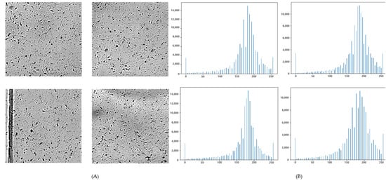
Figure 1.
Single-channel histogram graphs without modification of the SCB algorithm; N = 10: (A) four microscopy image samples; (B) Histograms corresponding to each image sample.
The details of the modified algorithm are as follows. When the lowest value among the pixel values of the image is expressed as P[min], the values of P[min] to N% or less, which are ambiguously expressed internal regions of the object, are determined as 0. To achieve this, the values of the two-dimensional matrix representing the image are converted into a one-dimensional vector arranged in ascending order by allowing duplicates. In this case, vectors are created for each channel.
After that, in order to process P[min] values lower than the N% of a random value selected by the user as the inner area of the object, the mask matrix that stores true for values lower than P[min] and false otherwise is used to determine the places that are true. The logic is executed to change to P[min]. Finally, a normalized image is obtained using the normalize function, and the normalization range is limited from 0 to P[avg]. P[avg] means the average value of the image histogram. The reason for doing this is that the object we are interested in has already been set to 0 by using the mask matrix, and only the low-density part or background remains in the rest of the object. That is, the background is compressed as much as possible by using P[avg], which occupies the greatest value in the background, and the histogram of the background is unified as much as possible based on this. This is to make it advantageous for the next step, image binarization operation. The pseudo code of the modified SCB is presented in Algorithm 1.
| Algorithm 1: Modified simplest color balance algorithm |
| percent = 10 //bottom 10% in histogram half_percent = percent/200.0 // double scale for subdivision, 1/100 -> 1/200 Red, Green, Blue = Split and save the RGB channels of the image // The logic below operates once in each of the Red, Green, and Blue channels. flat = reshape “channel” matrix array to vector array and sorted n_cols = length of flat low_val = flat[int(n_cols × half_percent)] // The part lower than low_val in the channel creates a matrix in which True and other False values are stored. low_mask <- if channel > low_val True else False matrix thresholded <- Stores a two-dimensional matrix in which low_val is assigned to a value lower than low_val. pixel_avg = average of thresholded histogram normalized = Normalize the thresholded channel to a value between 0 and b_cut. out_channel = After re-combining the three channels of Red, Green, and Blue, the grayscale image is returned. |
Most objects have different internal opacities depending on their density, and some have color due to other internal and external factors. Objects have various characteristics, but the most obvious characteristic with the highest influence in a given environment is that most of the inner area of the object has a slightly lower value than the background. As a result of running multiple experiments on the image used in the test in this study, the ideal value of N, which most clearly changes the pixel value of an object to 0, was set to 10 percent. Figure 2 shows the captured images after applying the modified SCB algorithm in accordance with the different N values used in the multi-run experiment.
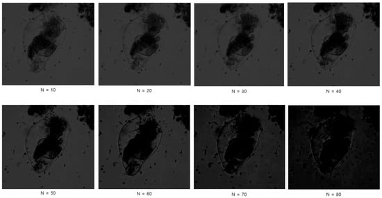
Figure 2.
Captured images after applying modified SCB algorithm with different N values.
To describe the histogram limitation used in the normalize function in more detail, since the pixel P[object] that can be estimated as an object in the test image occupies less area than the background pixel P[background] of the image, the average P of all pixels when [avg] is calculated is closer to P[background] than to P[object]. This is possible because we assume that the image quality is poor, so the contrast ratio is low and the light is evenly distributed over the observation area.
Using this characteristic, the histogram normalization range of the normalize function is limited to 0~P[avg] so that the background and object can be more clearly separated in the SCB algorithm. The result can be seen in Figure 3. At this point, the polarization of the object and the background proceeds, so even if the shapes of the graphs in Figure 3 are slightly different, there is no significant difference in their meaning. In the end, even if you do not go through the entire process proposed by the original SCB, you can separate the area of the object and then combine the matrices for each of the R, G, and B channels through the normalization function again. Then, the gray scale function is applied to the corresponding image. As can be seen when comparing Figure 3 and Figure 4, even if the histogram is restricted and normalized, there is no significant change in the graph shape of the original image and the normalized image. As shown in the graph in Figure 4, gray scale images can be flexibly applied even in situations where the P[max] of a specific channel is high due to the presence of a region biased toward a specific color in the image. Therefore, we did not use a single channel, but used a gray-scaled image. Finally, binarization is performed in the next step using a two-dimensional matrix that has been gray-scaled.
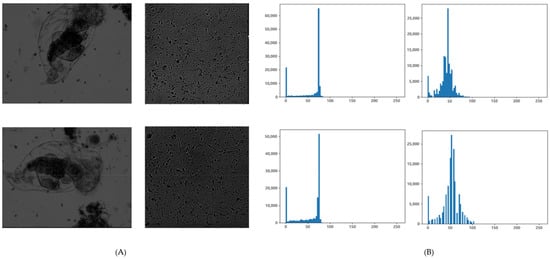
Figure 3.
1000× zoom microscopy image with limited histogram and histogram graph, N = 10: (A) four microscopy image samples; (B) Histograms corresponding to each image sample..
Figure 4.
Superimposed images of RGB and gray-channel histograms for Figure 3A.
3.2. Image Binarization
Threshold-based binarization was performed to clearly express the object found in the image output through the SCB algorithm. A general threshold application technique makes a relatively small part 0 and a large part 255 based on the threshold. For actual implementation, the widely used OpenCV was used. In this case, OpenCV’s contours function found an object based on the white area in the binarized image. To cope with this, we reversely applied 0 and 255, which are applied as threshold standards during binarization. That is, a binarized image is obtained in which a portion lower than the threshold value is expressed as 255, and a portion higher than the threshold value is ex-pressed as 0. Figure 5 shows the binarization of the image histogram based on the threshold value for the image restricted to P[object]~P[avg]. In this case, even though the SCB was applied according to the given image, it can be seen that the object detected by the SCB was not completely binarized according to the threshold value.
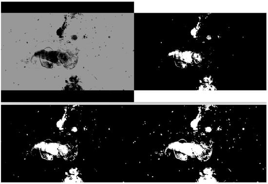
Figure 5.
Microscope images (1000× zoom) with binarization (top left: SCB only, top right: 1/4, bottom left: 1/2, bottom right: 3/4).
From Figure 5, it can be seen that the degree of object capture varies when the threshold value passed to the threshold function is 1/4, 1/2, or 3/4. From Figure 5 and Table 1, it was confirmed that the higher the threshold, the more objects were detected in detail. However, it was confirmed that the process of extracting an appropriate threshold value is necessary because an incorrect pixel area is detected when the threshold value is too large.

Table 1.
Number of objects detected by different threshold values.
3.3. Subsection
In object detection, functions related to contour provided by OpenCV were used. Contour generally represents contour lines, and it is a very effective function for extracting the area of the object expressed in white from the binarized image. You can use the find-contours function to detect the outer part of an object. If you connect the outer line of the object through this, you can know the value of its inner size. Finally, according to the obtained internal size value, it is checked whether the object the user wants to detect is correct.
In order to accurately find the object of interest through the method proposed in this study, we used a method of pre-defining the size of the object to be detected. In the case of an image at 300× magnification in Figure 6, the captured area is 0.3 mm wide and 0.3 mm long. Using this value, it is possible to inversely calculate the size of the floating object in the image. In the case of the 1000× magnification image in Figure 6, the size of the floating object can be estimated through the average size value of the bacteria present in the image. Floating objects in the image of Figure 6 are the results of detecting objects with a size between 10 and 60 in this way. We drew a blue box around the object using the detected object’s center coordinate value and wrote the object’s size and description in the upper left corner.
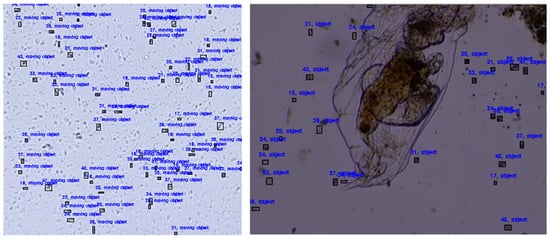
Figure 6.
Object detection results in images at 300× magnification (left) and 1000× magnification (right).
In general, in order to use machine learning, clear characteristics of the things to be detected are required, but it is difficult to extract features from the objects to be detected from the test image, and the number of features that can be extracted is very limited. In such an environment, it can be a very difficult task to apply machine learning, so the proposed detection algorithm can perform better.
3.4. Object Tracking
It was explained in Section 3.3 that an object can be specified from the binarized image obtained in Section 3.2. For the next step, if we give a unique ID value that can distinguish extracted objects and we continuously find pixels that can be inferred as objects corresponding to IDs in the frame being connected, we can track the objects of interest in the entire video.
For this, we used the connectedComponentsWithStats function provided by OpenCV. Using this, we proceeded to label the areas with the size suggested in Section 3.3 among the white areas obtained in Section 3.2. In the first frame, a tracker was allocated to the labeled areas, and then in the next frame, labeling was applied in the same way. Among the areas to which the label was applied, the area determined to be the same object as the one found in the previous frame was stored in the corresponding tracker. The tracker defines the state of the object based on the information of the labeled area allocated to each frame, and the details of the information can be checked in Table 2.
Table 2.
The details of the information checked by the tracker.
From the first frame to the last frame, the tracker has information on the areas for each frame that are most similar to the labeled area allocated in the first frame. The information stored in this tracker can be displayed by overlaying a specific mark on every frame of the original video. In this way, the tracker appears to keep tracking the object. Figure 7 is a flowchart of the operation flow of the tracking algorithm. The object-tracking algorithm tracks the moving path of an object by accumulating tracker information at every frame. The information stored during tracking includes the coordinates of the center of an object, its size, and the distance of each object’s center coordinates.
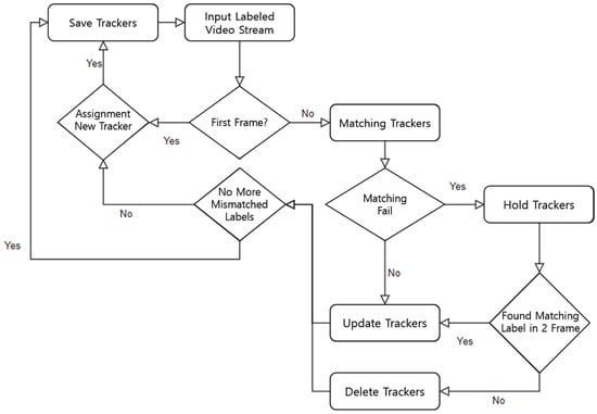
Figure 7.
Object-tracking algorithm.
In the first frame, in order to save the information of detected objects, it is assumed that all objects are in a stationary state and then the information is saved. From the second frame, when tracker matching starts, the ratio of the size similarity and length of objects is converted into scores, and then candidate groups higher than a certain threshold value are saved as the next tracker candidate. After removing trackers that fail to match during tracker matching, an inverse calculation is performed based on the remaining tracker information to analyze the activity, state, and distance information of the object.
When the analysis is finally finished, the movement path and state of the object are expressed in lines and colors in each frame using information from the tracker.
As a result of tracking the movement of the object and the path it moved through, the method described above is shown in Figure 8.
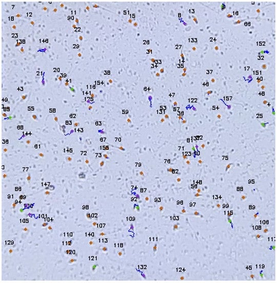
Figure 8.
Captured image of the object-tracking process.
4. Evaluation
In this section, we present experimental results to evaluate the proposed scheme. For the algorithm performance evaluation, AMD’s Ryzen 5 5600X was used, and all codes were written using Python and OpenCV.
In addition, 40 videos of similar types with noise collected for performance tests were classified and utilized to proceed with each test.
As a method of evaluating our proposed algorithm, the following method was used. The most widely used, precision-recall, was used for object detection. The object-tracking part calculates the ratio of how much the tracker maintains tracking and catches the wrong object in the entire frame, converts it into a percentage, and expresses it as the loss. For the object detection verification method, a random frame was selected from the entire image and the result obtained through the algorithm was compared with the result directly detected by a person and verified. In the case of tracking, a black square box was drawn at the coordinates where the tracker was located on the algorithm result screen to check if there was an error in the square. Figure 9 is a picture comparing the resulting image created by the algorithm with the red square box image drawn by a person for three of the images used for verification. We drew a square box to make tracking verification easier. The full verification result is shown in Table 3 below.
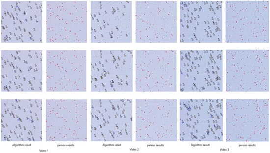
Figure 9.
Comparison of the square box image drawn by a person and the proposed scheme.
Table 3.
Precision-recall of object detection and loss-of-object tracking.
The strength of our proposed algorithm is that, when compared with the validation part of other reference papers, the same results were obtained for the same input, and even faster results were obtained without using a predefined training dataset. Table 4 below summarizes the time it took for our proposed algorithm to detect an object and output the result to the screen. The number of detected objects according to the time taken for each frame was written, and the time was written up to the second decimal place. In the case of the first frame, it took some time while reading the video, and there were some irregular measurements in the middle. However, it can be seen that on average, a very small time of 0.02 s was required.
Table 4.
Time required for each frame and number of detected objects.
Figure 10 is the result of comparing the performance of the proposed scheme with other algorithms. In each proposed method, the characteristics of the object to be detected are different. However, when trying to detect a large number of objects, comparing the time required to derive a result is very meaningful for the performance verification of the proposed method. As a comparison criterion, the computation time required to detect multiple objects was compared.
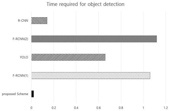
Figure 10.
The result of comparing the performance of the proposed scheme with that of other methods.
In the reference comparing the cases of F-RCNN(1) and YOLO, it was mentioned that each method takes 32 fps and 20 fps [5]. When 1 s is 30 fps, it can be seen that 32 fps and 20 fps are converted to 1.06 s and 0.66 s, respectively. For R-CNN, it was stated that the average detection time of the photos used in the test was 0.14 s, but it was only written for a single object [16]. When F-RCNN(2) was used, it was said that particles with a higher mobility were detected within 1.12 s [15]. Lastly, our proposed algorithm had an average processing time close to 0.02 s, indicating that it is relatively improved in real-time processing compared to other proposed machine-learning methods.
5. Conclusions
Finding an object of interest in an image and making an important judgment based on it has emerged as a very important research topic in recent years. Given this situation, we proposed a technique for tracking a moving object of interest in a noisy video to devise a technique that can build training data for machine learning. To track an object without a separate data set in such an environment, we designed an object detection and tracking algorithm based on a modified simplest color balance technique. The proposed method unifies the image information corresponding to the object to be detected through the SCB algorithm. In this paper, we adopted the idea of collectively minimizing values in a certain low range in the SCB algorithm. After applying the modified SCB algorithm to the image based on the idea, a binarization algorithm was applied to determine the exact object to be found. Finally, in order to track the object in the subsequent video, the label was displayed on the white bundle that was determined as the object in the frame unit. As a result, the detection accuracy of ambiguous objects was over 95%. The approach also reduced the tracking loss rate to 10%.
Our study can be used to distinguish and track objects that users want, excluding various unnecessary objects and very small objects present in micro-fields, and this study can be used in various fields related to cell research.
As a future work, we are planning to enhance the clarity of the input video itself by eliminating the unnecessary noise object. This might help improve the performance of object recognition in noisy videos.
Author Contributions
Methodology, H.-W.L.; validation, O.B.; investigation, J.L.; writing—original draft preparation, H.K.; supervision, C.-P.H. All authors have read and agreed to the published version of the manuscript.
Funding
This research was supported by the MIST (Ministry of Science, ICT), Korea, under the National Program for Excellence in SW, and was supervised by the IITP (Institute of Information and Communications Technology Planning and Evaluation) in 2022 (2019-0-01834).
Institutional Review Board Statement
Not applicable.
Informed Consent Statement
Not applicable.
Data Availability Statement
Not applicable.
Conflicts of Interest
The authors declare no conflict of interest.
References
- Lu, S.; Wang, B.; Wang, H.; Chen, L.; Linjian, M.; Zhang, X. A real-time object detection algorithm for video. Comput. Electr. Eng. 2019, 77, 398–408. [Google Scholar] [CrossRef]
- Wageeh, Y.; Mohamed, H.E.D.; Fadl, A.; Anas, O.; El Masry, N.; Nabil, A.; Atia, A. YOLO fish detection with Euclidean tracking in fish farms. J. Ambient Intell. Humaniz. Comput. 2021, 12, 5–12. [Google Scholar] [CrossRef]
- Lin, S.D.; Chang, T.; Chen, W. Multiple Object Tracking using YOLO-based Detector. J. Imaging Sci. Technol. 2021, 65, 40401-1. [Google Scholar] [CrossRef]
- Krishna, N.M.; Reddy, R.Y.; Reddy, M.S.C.; Madhav, K.P.; Sudham, G. Object Detection and Tracking Using Yolo. In Proceedings of the 2021 Third International Conference on Inventive Research in Computing Applications(ICIRCA), Coimbatore, India, 2–4 September 2021; pp. 1–7. [Google Scholar]
- Yang, H.; Liu, P.; Hu, Y.; Fu, J. Research on underwater object recognition based on YOLOv3. Microsyst. Technol. 2021, 27, 1837–1844. [Google Scholar] [CrossRef]
- Chen, J.W.; Lin, W.J.; Cheng, H.J.; Hung, C.L.; Lin, C.Y.; Chen, S.P. A smartphone-based application for scale pest detection using multiple-object detection methods. Electronics 2021, 10, 372. [Google Scholar] [CrossRef]
- Montalbo, F.J.P. A Computer-Aided Diagnosis of Brain Tumors Using a Fine-Tuned YOLO-based Model with Transfer Learning. KSII Trans. Internet Inf. Syst. (TIIS) 2020, 14, 4816–4834. [Google Scholar]
- Yüzkat, M.; Ilhan, H.O.; Aydin, N. Multi-model CNN fusion for sperm morphology analysis. Comput. Biol. Med. 2021, 137, 104790. [Google Scholar] [CrossRef]
- Yang, H.; Kang, S.; Park, C.; Lee, J.; Yu, K.; Min, K. A Hierarchical deep model for food classification from photographs. KSII Trans. Internet Inf. Syst. (TIIS) 2020, 14, 1704–1720. [Google Scholar]
- Stojnić, V.; Risojević, V.; Muštra, M.; Jovanović, V.; Filipi, J.; Kezić, N.; Babić, Z. A Method for Detection of Small Moving Objects in UAV Videos. Remote Sens. 2021, 13, 653. [Google Scholar] [CrossRef]
- Ibraheam, M.; Li, K.F.; Gebali, F.; Sielecki, L.E. A Performance Comparison and Enhancement of Animal Species Detection in Images with Various R-CNN Models. AI 2021, 2, 552–577. [Google Scholar] [CrossRef]
- Long, K.; Tang, L.; Pu, X.; Ren, Y.; Zheng, M.; Gao, L.; Song, C.; Han, S.; Zhou, M.; Deng, F. Probability-based Mask R-CNN for pulmonary embolism detection. Neurocomputing 2021, 422, 345–353. [Google Scholar] [CrossRef]
- Wu, Q.; Feng, D.; Cao, C.; Zeng, X.; Feng, Z.; Wu, J.; Huang, Z. Improved Mask R-CNN for Aircraft Detection in Remote Sensing Images. Sensors 2021, 21, 2618. [Google Scholar] [CrossRef] [PubMed]
- Zhu, R.; Cui, Y.; Hou, E.; Huang, J. Efficient detection and robust tracking of spermatozoa in microscopic video. IET Image Process. 2021, 15, 3200–3210. [Google Scholar] [CrossRef]
- Somasundaram, D.; Nirmala, M. Faster region convolutional neural network and semen tracking algorithm for sperm analysis. Comput. Methods Programs Biomed. 2021, 200, 105918. [Google Scholar] [CrossRef] [PubMed]
- Zhang, N.; Feng, Y.; Lee, E.J. Activity Object Detection Based on Improved Faster R-CNN. J. Korea Multimed. Soc. 2021, 24, 416–422. [Google Scholar]
- Shen, J.; Liu, N.; Sun, H.; Tao, X.; Li, Q. Vehicle Detection in Aerial Images Based on Hyper Feature Map in Deep Convolutional Network. KSII Trans. Internet Inf. Syst. (TIIS) 2019, 13, 1989–2011. [Google Scholar]
- Ilhan, H.O.; Serbes, G.; Aydin, N. Automated sperm morphology analysis approach using a directional masking technique. Comput. Biol. Med. 2020, 112, 103845. [Google Scholar] [CrossRef]
- Chang, V.; Heutte, L.; Petitjean, C.; Härtel, S.; Hitschfeld, N. Automatic classification of human sperm head morphology. Comput. Biol. Med. 2017, 84, 205–216. [Google Scholar] [CrossRef]
- Ilhan, H.O.; Serbes, G. Sperm morphology analysis by using the fusion of two-stage fine-tuned deep network. Biomed. Signal Process. Control 2021, 71, 103246. [Google Scholar] [CrossRef]
- Limare, N.; Lisani, J.L.; Morel, J.M.; Petro, A.B.; Sbert, C. Simplest color balance. Image Process. Online (IPOL) 2011, 1, 297–315. [Google Scholar] [CrossRef]
- Urbano, L.F.; Masson, P.; VerMilyea, M.; Kam, M. Automatic tracking and motility analysis of human in time-lapse images. IEEE Trans. Med. Imaging 2016, 36, 792–801. [Google Scholar] [CrossRef] [PubMed]
- Jati, G.; Gunawan, A.A.; Lestari, S.W.; Jatmiko, W.; Hilman, M.H. Multi-sperm tracking using Hungarian Kalman filter on low frame rate video. In Proceedings of the 2016 International Conference on Advanced Computer Science Information Systems(ICACSIS), Malang, Indonesia, 15–16 October 2016; pp. 530–535. [Google Scholar]
- Ilhan, H.O.; Yuzkat, M.; Aydin, N. Sperm Motility Analysis by using Recursive Kalman Filters with the smartphone based data acquisition and reporting approach. Expert Syst. Appl. 2021, 186, 115774. [Google Scholar] [CrossRef]


Disclaimer/Publisher’s Note: The statements, opinions and data contained in all publications are solely those of the individual author(s) and contributor(s) and not of MDPI and/or the editor(s). MDPI and/or the editor(s) disclaim responsibility for any injury to people or property resulting from any ideas, methods, instructions or products referred to in the content. |
© 2023 by the authors. Licensee MDPI, Basel, Switzerland. This article is an open access article distributed under the terms and conditions of the Creative Commons Attribution (CC BY) license (https://creativecommons.org/licenses/by/4.0/).