Article

Real-Time, Model-Agnostic and User-Driven Counterfactual Explanations Using Autoencoders

by
Jokin Labaien Soto
1,2,*,
Ekhi Zugasti Uriguen
2 and
Xabier De Carlos Garcia
1
1
Ikerlan Technology Research Centre, Basque Research and Technology Alliance (BRTA), Pº J.M. Arizmediarrieta, 2, 20500 Arrasate-Mondragón, Spain
2
Data Analysis and Cybersecurity Group, Mondragon University, Goiru Kalea, 2, 20500 Arrasate-Mondragón, Spain
*
Author to whom correspondence should be addressed.
Appl. Sci. 2023, 13(5), 2912; https://doi.org/10.3390/app13052912
Submission received: 3 February 2023 / Revised: 17 February 2023 / Accepted: 17 February 2023 / Published: 24 February 2023
(This article belongs to the Section Computing and Artificial Intelligence)

Abstract

:
Explainable Artificial Intelligence (XAI) has gained significant attention in recent years due to concerns over the lack of interpretability of Deep Learning models, which hinders their decision-making processes. To address this issue, counterfactual explanations have been proposed to elucidate the reasoning behind a model’s decisions by providing what-if statements as explanations. However, generating counterfactuals traditionally involves solving an optimization problem for each input, making it impractical for real-time feedback. Moreover, counterfactuals must meet specific criteria, including being user-driven, causing minimal changes, and staying within the data distribution. To overcome these challenges, a novel model-agnostic approach called Real-Time Guided Counterfactual Explanations (RTGCEx) is proposed. This approach utilizes autoencoders to generate real-time counterfactual explanations that adhere to these criteria by optimizing a multiobjective loss function. The performance of RTGCEx has been evaluated on two datasets: MNIST and Gearbox, a synthetic time series dataset. The results demonstrate that RTGCEx outperforms traditional methods in terms of speed and efficacy on MNIST, while also effectively identifying and rectifying anomalies in the Gearbox dataset, highlighting its versatility across different scenarios.

1. Introduction

Recently, the field of Artificial Intelligence (AI) has witnessed significant progress with the rise of Deep Learning (DL) techniques. These methods have shown great success in various areas, but they also have limitations, particularly in terms of interpretability and robustness. DL models tend to be complex, with millions of parameters, which can make it challenging to understand the reasoning behind their predictions. Additionally, these models are trained on historical data that may contain biases, resulting in unfair and incorrect decisions. These limitations are especially problematic in industrial domains, where a lack of trust in the models’ predictions can lead to the use of less effective but more interpretable methods. To address these limitations, research in the area of Explainable Artificial Intelligence (XAI) has gained traction recently. The goal of XAI is to find a balance between model effectiveness and interpretability, allowing for understanding of the decision-making processes of AI models.
In recent years, many methods have been proposed regarding the explainability of ML models. Some of these methods use rules to explain other models and are called rule-based methods, such as Anchors [1] or RuleFit [2]. In a different way, attribution-based methods attempt to attribute an influence score to each input variable. These methods are the most used ones in the XAI community, and the influence attributions can be computed in many ways. One way uses perturbation-based methods, such as SHAP [3] or LIME [4], which make small variations in the input variables of a model to see how the output varies. Another way is by gradient-based methods, such as Integrated Gradients [5] for example, which compute the attributions as a function of the partial derivatives of the target with respect to the input features.
Other methods for explaining model decisions utilize counterfactual explanations [6]. Counterfactual explanations are presented in the form of conditional statements, which aim to answer the question “what would happen if…?”. In the context of Machine Learning, a counterfactual explanation describes the modifications that must be made to the input of a model in order to alter its prediction. The properties of counterfactual explanations may vary depending on the particular context in which they are employed [7]. In summary, the following are the general properties that a counterfactual explanation should meet, according to [7]:
  • Data closeness: Given an input x , the counterfactual explanation x c f has to be a minimal perturbation of x , i.e.,
    x x c f .
    Related to data closeness [7] also mentions sparsity. However, this property can be a challenge when working with continuous variables because it may not be possible to find a parsimonious explanation by only modifying a few features.
  • User-driven: The counterfactual explanation has to be user-driven, meaning that the user can indicate whether the class y c f , to which a counterfactual x c f belongs, can be specified. That is, given a black-box model f ( · )
    f ( x c f ) = y c f .
    Otherwise, in multiclass problems, for example, the changes would only be directed to the closest class, excluding explanations for other classes. Note that this property also ensures the validity property of [7].
  • Amortized inference: The counterfactual explanations have to be straightforward, without solving an optimization problem for each input to be changed. In this way, the explanation model should learn to predict the counterfactual. The algorithm needs to quickly calculate a counterfactual for any new input x . Otherwise, the process of generating explanations is time-consuming.
  • Data manifold closeness: In addition to satisfying the property of data closeness, a counterfactual instance has to be close to the distribution of the data ( p d a t a ), i.e., the changes have to be realistic, i.e.,
    x c f p d a t a .
  • Agnosticity: The generation of counterfactuals can be applied to any machine learning model without relying on any prior knowledge or assumptions about the model.
  • Black-box access: The generation of counterfactuals can be achieved with access to only the predict function of the black-box model.
In order to fulfill all these properties, it is necessary to design an algorithm that optimizes various aspects in the loss function. This loss function should penalize large changes, out-of-distribution counterfactuals, and counterfactual explanations that do not match the counterfactual label defined by the user. Thus, in this paper, we propose Real-Time Guided Counterfactual Explanations (RTGCEx), a model-agnostic algorithm that is capable of creating counterfactual explanations in real time through the use of autoencoders, by optimizing a loss function that takes into account all these properties.
The paper is organized as follows: In Section 2, we review the related works in the field. In Section 3, we present the proposed algorithm in detail. Section 4 describes the experimental framework used to evaluate RTGCEx. In Section 5, we present and analyze the results obtained from the experiments. Finally, in Section 6, we summarize the main contributions of this work and discuss directions for future research.

2. Related Work

The provision of counterfactual explanations in machine learning models is becoming increasingly important in the field of XAI (eXplainable Artificial Intelligence) because it resembles human reasoning, where we often use what-if statements when providing an explanation for an event [8]. However, most classical methods for generating counterfactual explanations involve solving an optimization problem for each input datum x to generate the counterfactual explanation x c f , which can be time-consuming and result in explanations that are not straightforward.
One of the first methods proposed for this purpose was CEM [9], which generates minimal changes to an input that change the model prediction to its nearest class. Similarly, Van Looveren et al. [10] introduced a term regarding class prototypes to speed up the explanation process and allow for the specification of the target class. However, these methods still involve solving optimization problems and thus, the explanations are not straightforward. More recent proposed methods, such as PIECE [11], generate more plausible counterfactual explanations and also produce semi-factual explanations, which are the largest possible feature modifications made to the input without changing the classification [12]. However, PIECE is only applicable for CNN-based models. Another recent method, DiCE [13], generates a set of k different counterfactual explanations for each input, but is limited to binary classification problems.
The limitations of these methods in terms of time-consuming and non-straightforward explanations have led to the development of amortized inference methods, which consist of models trained to generate counterfactual explanations instantaneously. These are typically generative models, such as Generative Adversarial Networks (GANs) [14,15] or Variational Autoencoders (VAEs) [16]. However, these methods also have their own limitations, such as the difficulty of training GANs, instability or non-convergence [17], or the lower quality reconstructions of VAEs. Recently, it has been proposed to use a simple AE to generate counterfactual explanations. Balabsubramanian et al. [18] propose a simple method that considers binary classification problems. In this method, the counterfactual explanations are obtained by minimally changing the latent representation of the encoder so that the prediction given by a classifier f ( · ) to the decoded sample reaches a predefined target probability p. Additionally, most of these methods have focused on image or tabular data rather than time series data.

3. Real-Time Guided Counterfactual Explanations

Real-Time Guided Counterfactual Explanations (RTGCEx) is a model-agnostic algorithm that uses an autoencoder for generating real-time counterfactual explanations for a given black-box model f ( · ) .
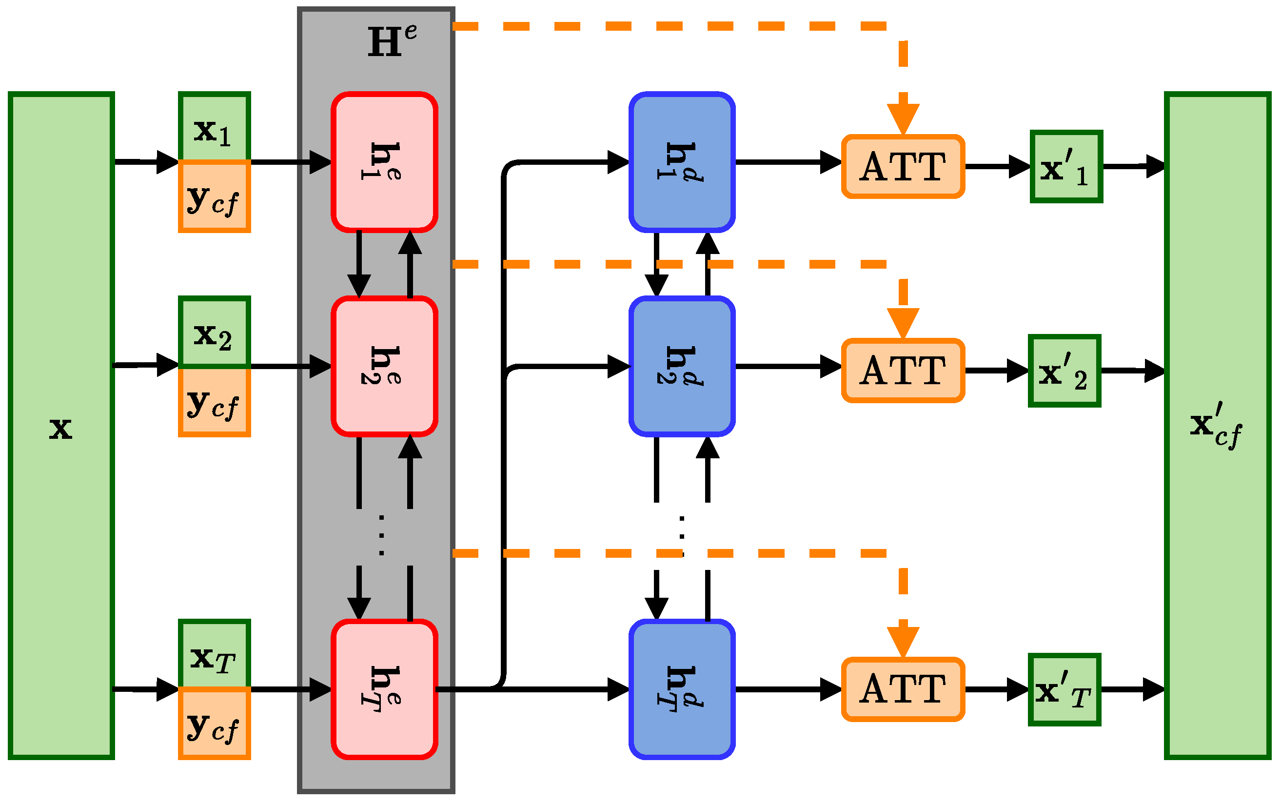
In the RTGCEx framework, as depicted in Figure 1, the generation of counterfactual explanations is achieved through the interaction of three components: a Generator (G), an Autoencoder (AE), and a black-box model  f ( · ) . The black-box model f ( · ) can be any machine learning model, as long as the predict function is accessible. As discussed in Section 1, the counterfactual explanations produced by RTGCEx must satisfy certain criteria, such as data closeness, closeness to the data distribution, and user-specified explanations, among others. To ensure that these properties are upheld, given a trained black-box model f ( · ) , RTGCEx involves two phases of training:
  • Autoencoding phase:
Involves training an autoencoder by minimizing a loss function that measures the distance between the original samples x D , where D denotes the dataset on which f ( · ) has been trained, and their reconstructions x .
  • Counterfactual generation phase:
This phase involves training G to ensure the properties discussed in the previous section, i.e.,
f ( x ) x , f ( G ( x ) ) = y c f and x c f ρ d a t a .
For this purpose, only the weights corresponding to G are trained, but the training makes use of the capacities that f ( · ) has to classify the inputs and the capacities that AE has to reconstruct the inputs that are similar to the ones learned during the training phase. Training G involves minimizing the following loss function:
L G , f , AE ( x , x c f , x c f y c f , y c f ) = α · L G ( x , x c f ) + β · L f ( y c f , y c f ) + γ · L AE ( x c f , x c f )
where α , β , γ > 0 are regularization coefficients. The first term, L G ( x , x c f ) , measures the distance between x and the counterfactual sample x c f , which ensures that the changes are minimal. The second term, L f ( y c f , y c f ) , measures the distance between the predefined counterfactual class y c f and the prediction given by f ( · ) to x c f , i.e., y c f , which ensures that the input x is changed to the class y c f defined by the user. Finally, the third term, L AE ( x c f , x c f ) , is the reconstruction error of the counterfactual instance x c f when using the AE. Because the AE has been trained with instances of the dataset D , the reconstruction error will be smaller when x c f is similar to the samples used in training, so L AE ( x c f , x c f ) penalizes unrealistic changes of the input x , ensuring the data manifold closeness property.

4. Experimental Framework

In this section, we present a description of the experimental setup. Below, we describe the datasets used, the models employed, and the evaluation metrics.

4.1. Datasets

  • MNIST.
The MNIST [19] dataset is a widely-used dataset in the machine learning community, specifically for the task of image classification. It consists of a total of 70,000 images, with 60,000 images being used for training and 10,000 images being used for testing. Each image is a 28 × 28 pixel grayscale image of a handwritten digit, labeled with the corresponding digit (from 0 to 9).
  • Gearbox.
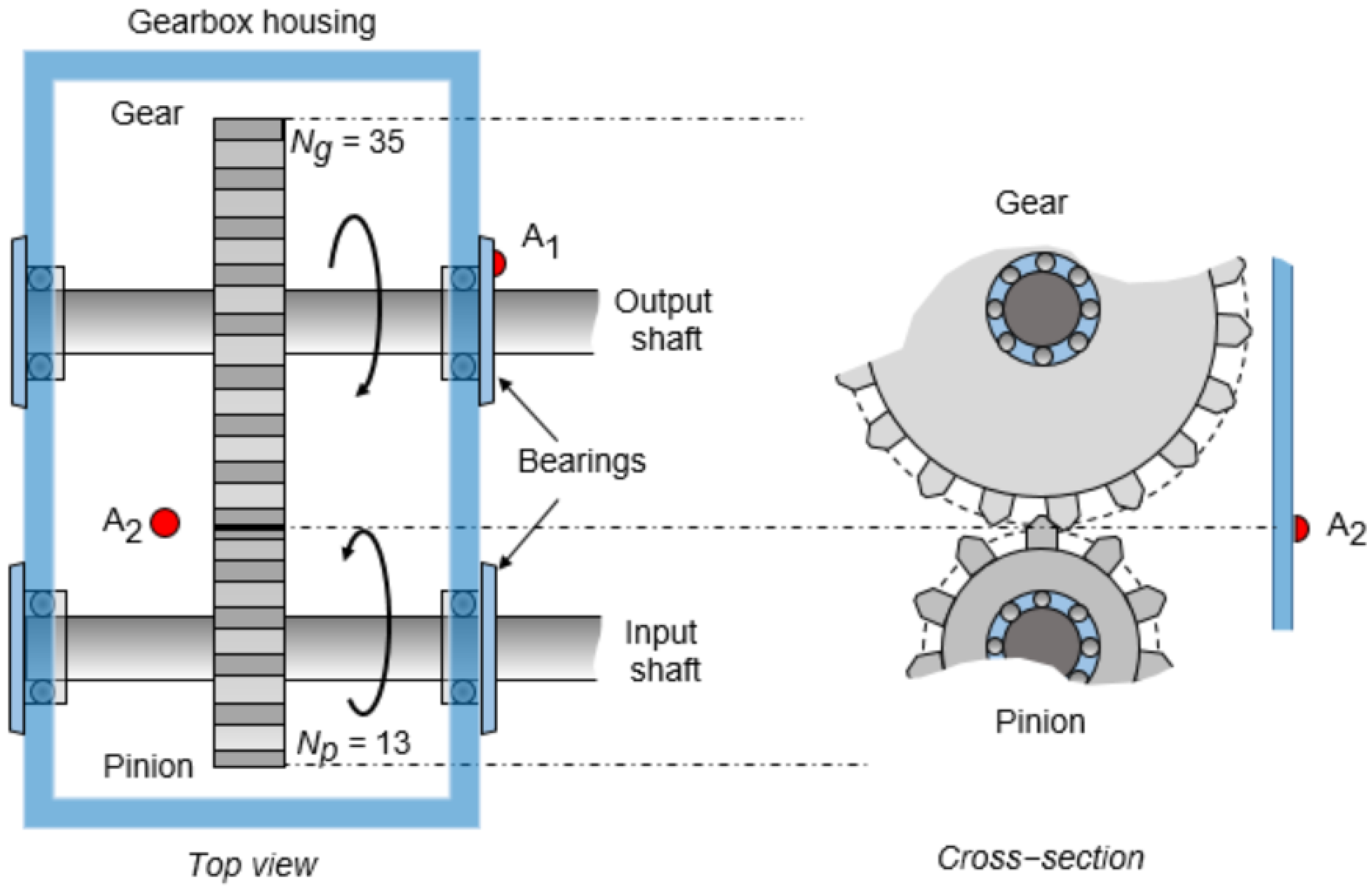
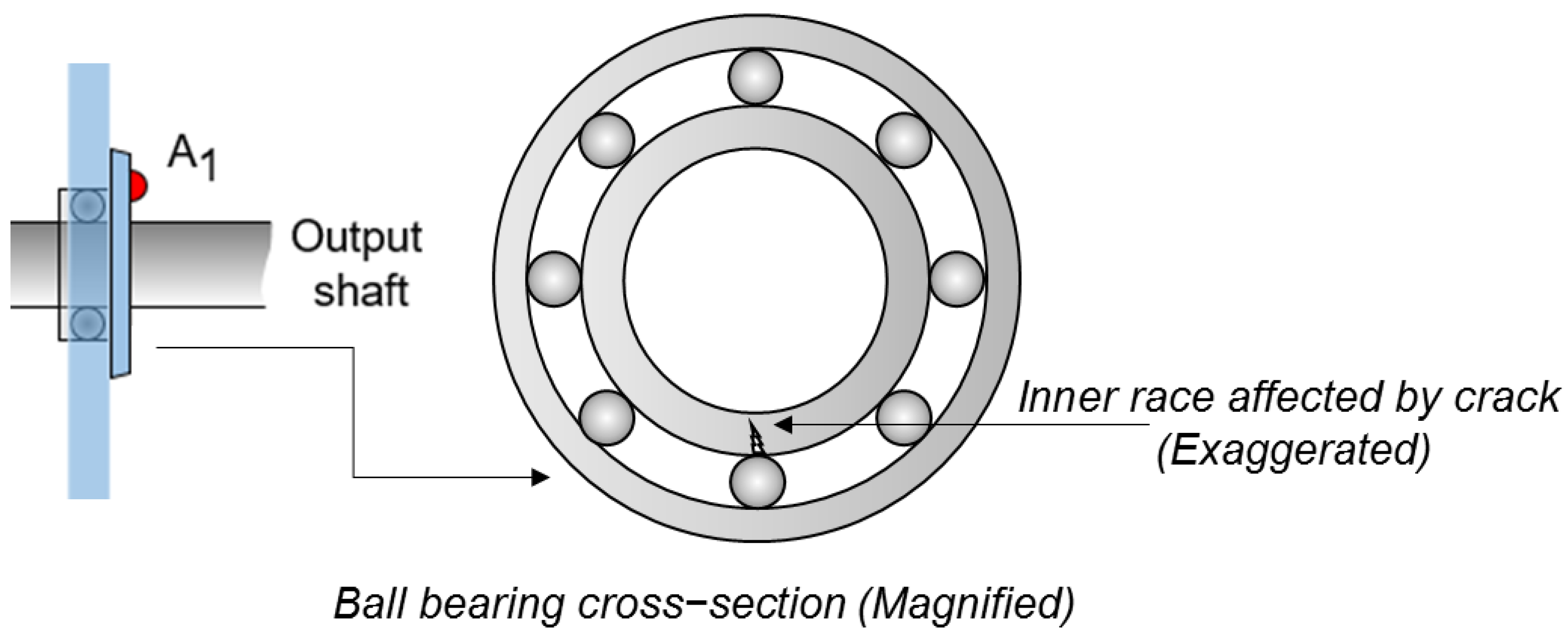
The Gearbox dataset is obtained from a gearbox vibration simulator [20]. The simulator generates vibration data for a gearbox with rotating axes that operate at a fixed speed. The overall operation of the rotatory machine is illustrated in Figure 2. The simulator considers an idealized gearbox in which the pinion is coupled to an input shaft connected to the primary engine, while the gear is connected to an output shaft. The shafts are supported by roller bearings located within the gearbox housing. The behavior of the bearings and gearbox housing is monitored using two accelerometers, labeled A1 and A2. In this research, we focus on analyzing the signals obtained from accelerometer A1, which records the contributions of the two shafts, as well as the coupled gear. Depending on the types of failures that can occur within the gearbox, these contributions can vary. In particular, we focus on faults caused by a crack in the inner race of the bearing (as shown in Figure 3). This type of fault generates high-frequency vibrations in the gearbox structure between the bearing and the response transducer.

4.2. Employed Models

As previously stated, RTGCEx consists of various sub-models. Here we present the architectures used for each use case for these sub-models.

4.2.1. MNIST

  • Black-box model.
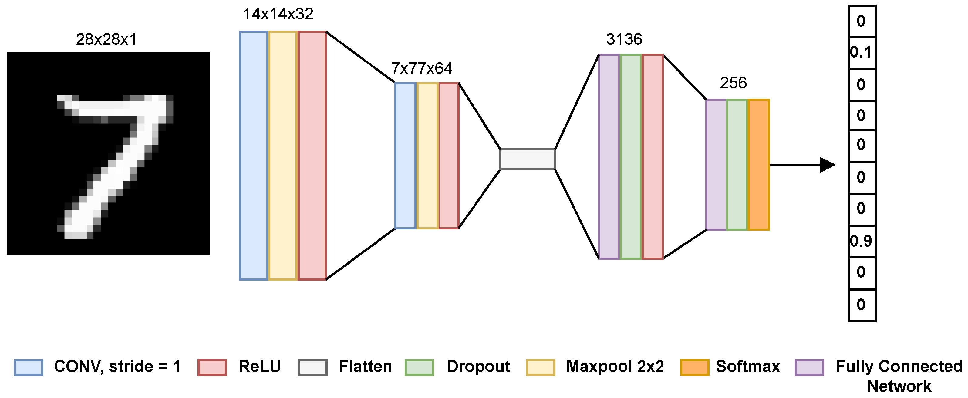
The black-box model f ( · ) used has the same architecture as the one used in [10]. That is, the model consists of two convolutional layers with 32 and 64 2 × 2 filters, respectively, with ReLU activation function. In addition, a 2 × 2 MaxPooling layer is applied after each convolutional layer to reduce dimensionality and avoid overfitting. Dropout with a fraction of 30% is applied during training. After the second MaxPooling layer, the output is flattened to apply a fully connected layer with 256 units, ReLU activation function, and 50% dropout. Finally, another fully connected layer with 10 units and a softmax activation function is used for classification. For more details, see Figure 4.
  • Autoencoder.
The encoder is composed of two convolutional layers with 32 and 64 2 × 2 filters, respectively, with ReLU activation function. The output of the second convolutional layer is flattened to feed a fully connected layer with 16 units, from which a 16-dimensional latent vector z is obtained. Then, this vector is fed to a fully connected layer that transforms the z vector into a vector of the same dimensionality as the flattened output of the second convolutional layer. This vector is reshaped into a 7 × 7 × 64 tensor to initialize the transposed convolutions. The decoder has three transpose convolution layers, with 64, 32, and one 2 × 2 filters, respectively. All the transpose convolutions are followed by a sigmoid function. For more details, see Figure 5.
  • Generator.
The architecture of the generator closely resembles that of the AE (see Figure 5), except that in this case the latent vector z is concatenated with the one-hot representation of the class to which the input has to be changed, i.e., y c f .

4.2.2. Gearbox

  • Black-box model.
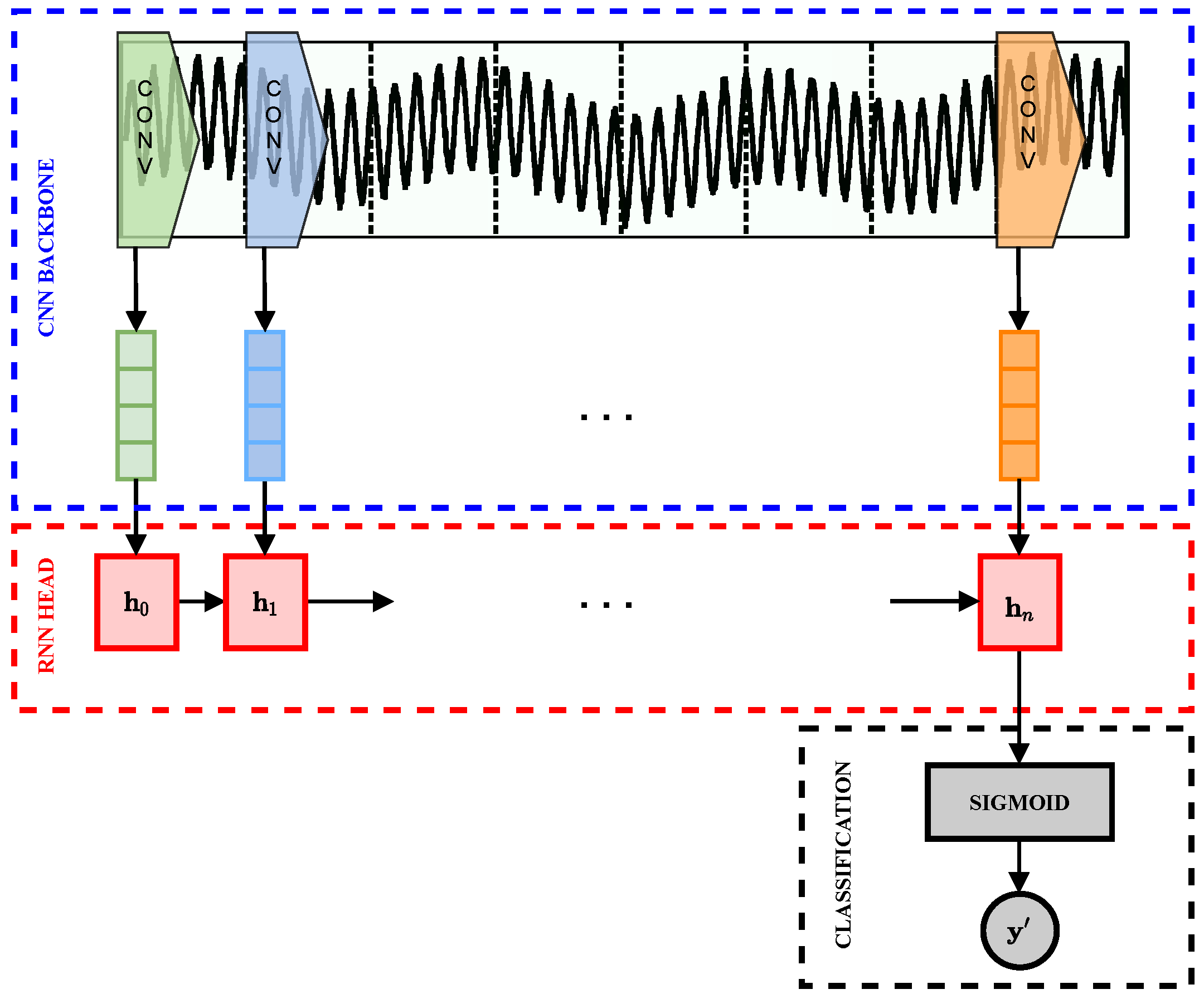
The proposed black-box model f ( · ) for the classification stage is illustrated in Figure 6. This model is based on the anomaly detection model proposed by Cañizo et al. [21], which is a combination of 1-Dimensional Convolutional Neural Networks (1D-CNN) with Recurrent Neural Networks (RNNs). The architecture is designed to be valid for both multivariate and univariate time series. The classificator f ( · ) is composed of three parts: the CNN backbone, the RNN head, and the classification head.
The CNN backbone, as shown in Figure 7, is composed of three convolutional blocks, each containing 1D-CNNs with a ReLU activation function, Batch Normalization, and Dropout regularization layers. The 1D-CNNs in the convolutional blocks are composed of 128, 64, and 32 filters, respectively, with a kernel length of 5 and a stride of 1. The proposed architecture processes the data in a window-based manner, whereby the input data x R L are divided into a sequence of T windows x = ( x 1 , , x T ) and the convolutional blocks are applied to each window separately, resulting in a vector of features F t for each time window x t . These extracted features are the inputs of the RNN head, which is composed of a Bi-LSTM layer that processes the features in chronological order in both directions, allowing for the identification of hidden temporal patterns within the extracted features. Finally, the last hidden state is input into a fully connected layer with a sigmoid activation function, and the final output is computed as
y = sigmoid ( W c h T + b c )
where W c and b c are the weights and bias of the fully connected layer, respectively.
  • Autoencoder.
The proposed Autoencoder (AE) is composed of a Bi-directional Long Short-Term Memory (Bi-LSTM) network with 128 hidden units for both the encoder and the decoder. The forward and backward hidden states of the encoder are concatenated to obtain the hidden state representation h t e = [ h e t , h e t ] , which contains the context information around time step t = 1 , , T . The last hidden state h T e is used as the vector representation z R d z , which contains the compressed information of the input sequence.
In a traditional sequence-to-sequence learning framework, the vector z is used by the decoder to transform it back into a sequence x = ( x 1 , , x T ) as close as possible to the encoder input x = ( x 1 , , x T ) . However, when dealing with long sequences, the latent representation z may not accurately capture all the information present in the input. To address this issue, attention mechanisms have been introduced to allow the decoder to focus on the most relevant encoder hidden states at each time step. In this work, an attention mechanism is used, whereby the attention weights are computed with an alignment score function. The attention weights at time-step t are calculated as:
α t , i = exp score h t d , h i e j = 1 T exp ( score h t d , h j e ) ,
s . t score h t d , h i e = ( h t d ) W a h i e ,
c t = i = 1 T α i , t h t e
where α t , i are the attention weights, which represent the importance that the input at position i has had over the output at time-step t, c t is the context vector, which is the sum of the hidden states weighted by the attention weights, and W a is the weight matrix to be learned. The final reconstruction of x t at time-step t is given by:
x t = sigmoid ( W b [ c t , h t d ] )
where W b is the weight matrix of a fully connected layer.
  • Generator.
For the generator to be able to make minimal changes in x that result in it being classified as a predefined counterfactual class y c f , the generator must consider both the time series data and the counterfactual class. To accomplish this, the proposed generator in Figure 8 is structured similarly to the autoencoder (AE) used for ensuring data manifold closeness, but with the added step of concatenating each input window x t with the counterfactual class y c f so that the information of the counterfactual class is included in each of the hidden states. That is, each input window x t now becomes [ x t , y c f ] .

4.3. Loss Functions

In both use cases, the optimization problem is similar, so the loss functions that we used in both cases are almost the same. As previously described, the training process consists of two phases:
  • Autoencoding phase: In this stage, we optimize a loss function with the aim of learning to reconstruct the inputs x from the training dataset. The loss function employed for this purpose is the mean squared error (see Equation (11)):
    L AE ( x , x ) = 1 N i = 1 N ( x ( i ) x ( i ) ) 2
    where N denotes the number of training samples.
  • Counterfactual generation phase: During this phase, the weights of the autoencoder and the black-box model are maintained constant, and the generator is optimized to minimize a loss function that incorporates three distinct terms (as shown in Equation (5)).
    -
    Data closeness loss: This loss function has to minimize the distance between the original samples x and counterfactuals x c f . Thus, we employ the mean squared error in both use cases:
    L G ( x c f , x c f ) = 1 N i = 1 N ( x c f ( i ) x c f ( i ) ) 2 .
    -
    Validity loss: This loss function has to ensure that the class given by the black-box model y c f matches the counterfactual class defined by the user, i.e., f ( x c f ) = y c f . As the MNIST use case is a multiclass problem and the Gearbox use case is a binary classification problem, we use different loss functions here.
    On the one hand, for MNIST, we used the categorical cross-entropy loss:
    L f ( y c f , y c f ) = 1 N i = 1 N j = 1 C y c f , j ( i ) · log ( y c f , j ( i ) )
    where y c f ( i ) is the one-hot encoded ground truth label and C is the number of classes.
    On the other hand, for the Gearbox use case, we used the binary cross-entropy loss:
    L f ( y c f , y c f ) = 1 N i = 1 N ( y c f ( i ) · log ( y c f ( i ) ) + ( 1 y c f ( i ) ) · log ( 1 y c f ( i ) ) )
    where y c f is 0 for normal data and 1 for anomalous data.
    -
    Data manifold closeness loss: This loss function ensures that the generated counterfactuals are close to the data manifold. Thus, it has to minimize the distance between the generated counterfactuals x c f and the reconstruction given by the AE for the counterfactuals x c f . Therefore, the loss used for this was the mean squared error:
    L AE ( x c f , x c f ) = 1 N i = 1 N ( x c f ( i ) x c f ( i ) ) 2 .

4.4. IM1 and IM2 Metrics

To assess the interpretability of the counterfactuals generated with each method, two metrics proposed by Van Looveren et al. [10], IM1 and IM2, have been used. On the one hand, IM1 measures the ratio between the reconstruction error of the counterfactual x c f using an AE specifically trained with instances of the counterfactual class ( AE y c f ) and using another AE trained with instances of the original class ( AE y ).
IM1 ( AE y c f , AE y , x c f ) : = x c f AE y c f ( x c f ) 2 2 x c f AE y ( x c f ) 2 2 + ϵ
A smaller value of IM1 means that the counterfactual instance is easier to reconstruct with the AE trained only with instances of the class y c f than with the AE trained only with instances of the original class t 0 . This means that the counterfactual instance is closer to the data manifold of the y c f class instances than to those belonging to the original class t 0 . On the other hand, IM2 measures how close the counterfactual instance is to the data manifold. To do so, it compares the reconstructions of the counterfactual instances when using an AE trained with instances of all classes (AE) and the AE trained with instances of the counterfactual class ( AE y c f ). To make the metric comparable across all classes, IM2 is scaled with the L 1 norm of x c f .
IM2 ( AE y c f , AE , x cf ) : = AE y c f ( x c f ) AE ( x c f ) 2 2 x c f 1 + ϵ
When the reconstruction of x c f by AE and by AE y c f is similar, IM2 is low. A lower value of IM2 makes the counterfactual instance more interpretable, because the data distribution of the counterfactual class y c f describes x c f equally well as the distribution over all classes.

5. Results and Discussion

This section analyzes the results obtained with RTGCEx in both the MNIST and Gearbox datasets.

5.1. MNIST

In order to train a generator to produce counterfactual explanations, it is necessary to first train both an autoencoder (AE) and a black-box model f ( · ) . The proper functioning of both the AE and the model f ( · ) is crucial for the generator to operate correctly. As depicted in Table 1, the performance of both the autoencoder and the black-box models was evaluated before training the generator. The autoencoder was evaluated using the mean squared error (MSE) on the test set, resulting in a value of 0.007. This suggests that the autoencoder is capable of accurately reconstructing the input data. On the other hand, the black-box model was evaluated using accuracy score, which resulted in a value of 0.991. This implies that the black-box model is able to correctly classify the majority of the images in the test set.
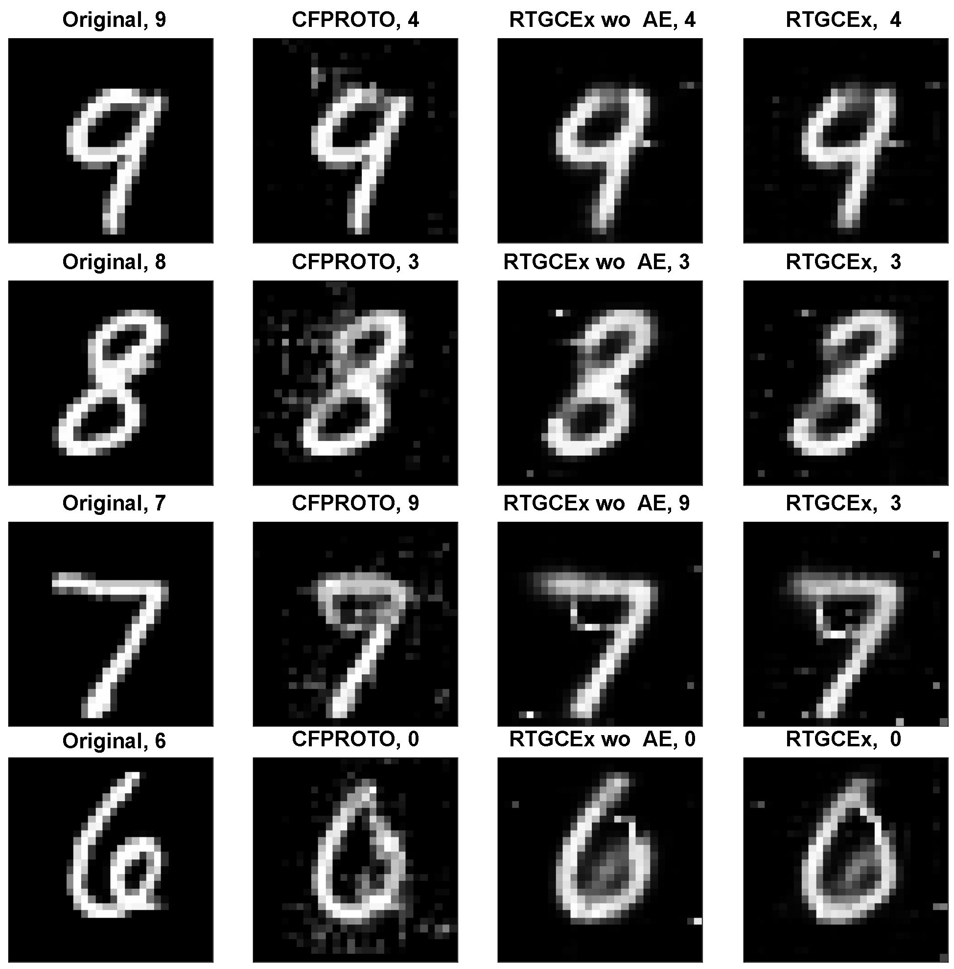
After training the generator, experiments were conducted to investigate the performance of the proposed RTGCEx method in comparison with a classical method, Counterfactual Prototype (CFPROTO). Additionally, the impact of the loss function was evaluated by comparing RTGCEx with its variant without the use of the AE. The results of these experiments are illustrated in Figure 9, which presents a selection of examples of the generated counterfactual instances. The original instances, along with their corresponding labels, are displayed in the first column, while the counterfactual instances generated by CFPROTO, RTGCEx without AE, and RTGCEx are displayed in the second, third, and fourth columns, respectively. The first row of the figure illustrates how each algorithm converts an original instance of the digit 9 into a 4. In this example, CFPROTO makes minimal modifications to a small part of the upper side of the 9 by removing a few pixels. On the other hand, RTGCEx without AE and RTGCEx make larger changes, but the final result appears more similar to a 4 compared with the counterfactual generated by CFPROTO. Similarly, in the second example, an 8 is converted into a 3, and it is observed that the counterfactual instances generated by RTGCEx without AE and RTGCEx are clearer than the one generated by CFPROTO. In the third example, a 7 is converted to a 9, and all methods produce counterfactual instances that closely resemble a 9, although the instance generated by CFPROTO may be more realistic. Lastly, in the fourth example, a 6 is changed to a 0 by removing the pixels of the lower circle of the 6 and adding new pixels to join the upper part, creating a complete circle.
The effectiveness of the proposed RTGCEx and RTGCEx without AE models were evaluated by generating counterfactual instances for each test sample. In order to ensure a fair comparison, the nearest prototype class y c f was first generated using CFPROTO, and then instances of the same class were generated using RTGCEx and RTGCEx without AE. The results of the evaluation are presented in Table 2, which shows the mean and interquartile range (IQR) of each method in terms of the metrics IM1, IM2, and speed. Following the criteria established for evaluation in [10], we multiplied the IM2 metric by 10.
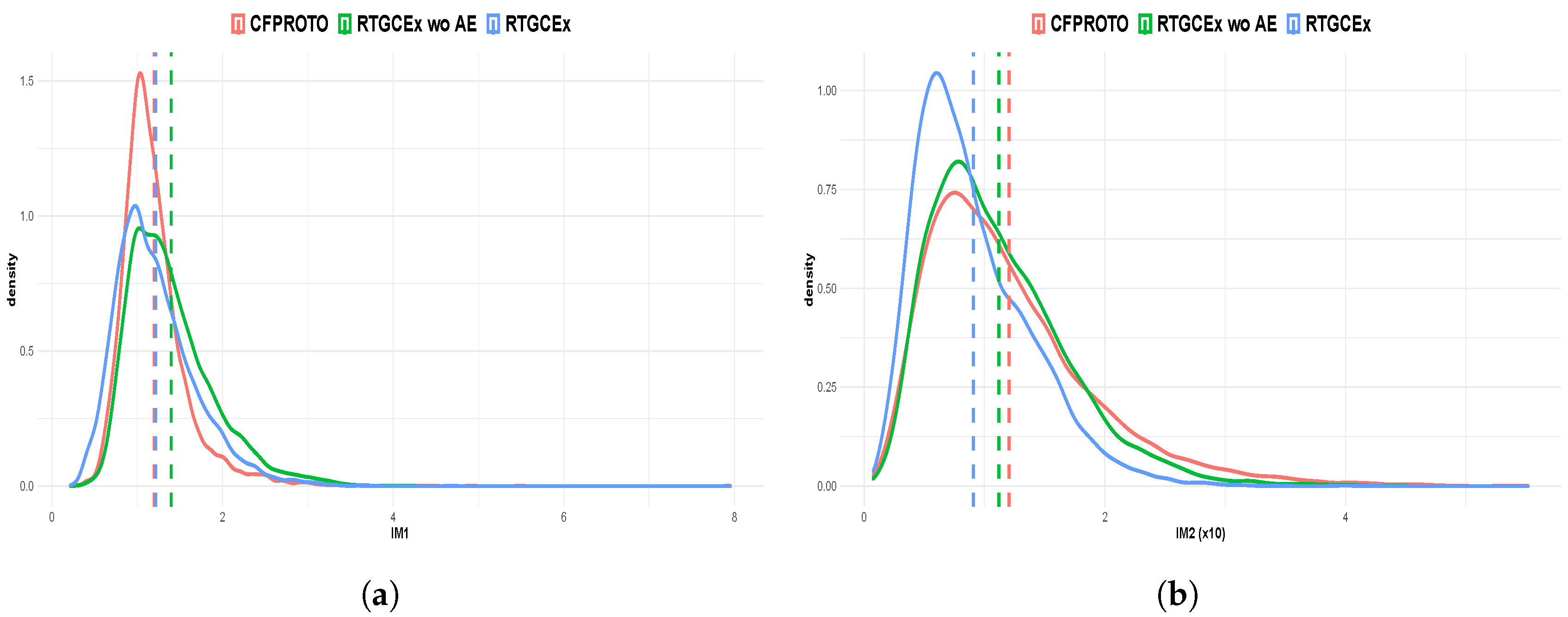
In terms of IM1, both CFPROTO and RTGCEx performed better than RTGCEx without AE. The results of CFPROTO and RTGCEx were similar, but CFPROTO had less variability, with an IQR of 0.39, compared with 0.58 for RTGCEx. For IM2, RTGCEx outperformed the other two algorithms. When comparing CFPROTO with RTGCEx without AE, it was found that the mean of the values obtained with RTGCEx without AE was 0.08 points lower than that of the values obtained with CFPROTO, and the variability was also lower. The RTGCEx without AE results were significantly improved by introducing a term that penalizes out-of-distribution changes, resulting in a decrease in mean IM2 values from 1.12 to 0.91 and a decrease in variability.
In terms of computational efficiency, CFPROTO took 17.40 s per iteration with a variability of 0.09 s, while RTGCEx without AE and RTGCEx took 0.14 s per iteration with a variability of 0.01 s. It should be noted that RTGCEx without AE and RTGCEx have the same architecture and thus take the same amount of time at inference.
In this research, the comparison of models is conducted by examining the distribution of IM1 and IM2 values, rather than using statistical tests on large samples. This approach is deemed more appropriate because the use of statistical tests on large samples can lead to p-values that are extremely small, which can result in the conclusion of support for results that have little practical significance [22]. We have a test set with 10,000 instances, and the distribution of the IM1 and IM2 values obtained from each method are shown in Figure 10. These distributions support the conclusions drawn from Table 2. Specifically, the means of IM1 values for CFPROTO and RTGCEx are similar, while those of RTGCEx without AE and RTGCEx have more variability. Additionally, the mean and variability of IM2 values is lower when using RTGCEx compared with the other methods.
Furthermore, these distributions allow for the drawing of numerical conclusions regarding the comparison of the models, such as the probability that a counterfactual instance will have lower values in terms of IM1 or IM2 when using one method versus another. These comparisons are shown in Table 3. For example, the value of 0.66 in the first row and second column of the table indicates that there is a probability of 0.66 that the IM1 value of an instance generated by CFPROTO will be less than an instance generated by RTGCEx without AE. Additionally, we can see that RTGCEx improves drastically over RTGCEx without AE, as an instance generated by RTGCEx has a probability of having lower IM1 and IM2 of about 0.75 compared with one generated with RTGCEx without AE. When comparing RTGCEx with CFPROTO, in terms of IM2, the probability of obtaining better counterfactual instances with RTGCEx is 0.62 with respect to CFPROTO. As for IM1, CFPROTO and RTGCEx have the same probability that the value will be lower using one method or the other.
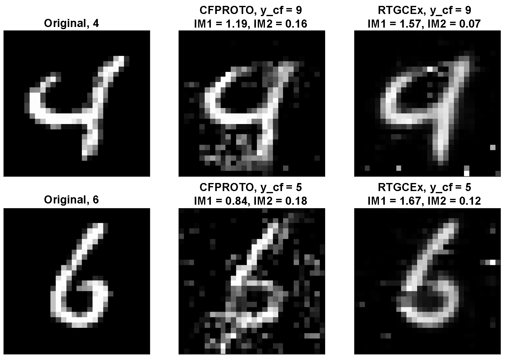
Upon analyzing the metrics used to measure the interpretability of counterfactual instances, we have found that IM1 does not always accurately reflect the interpretability of the instances. In some cases, a lower value of IM1 does not necessarily indicate that the counterfactual instances are more interpretable. To illustrate this point, we present two examples of counterfactual instances generated using CFPROTO and RTGCEx in Figure 11.
From the visual representation, it can be observed that the instances generated using CFPROTO appear to be less realistic than those generated using RTGCEx. This is reflected in the value of IM2, as instances generated by CFPROTO have a higher value of IM2 than those generated by RTGCEx. However, it is also worth noting that even though the instances generated by CFPROTO are not as realistic, in this case, their IM1 value is significantly lower than that of RTGCEx. In [23], the authors also found that two counterfactuals that were supposed to be similarly realistic exhibited a significant difference in the IM1 metric, with one having a notably smaller value than the other. This discrepancy highlights the limitations of using IM1 as the sole metric to measure the interpretability of counterfactual instances.

5.2. Gearbox

In order to evaluate the performance of the AE and the function f ( · ) , experimental analysis was conducted. The results of these experiments are presented in Table 4.
For the autoencoder, we employed the mean squared error (MSE) metric to evaluate its performance. The low MSE values obtained suggest that the autoencoder is able to accurately reconstruct the input samples. In addition, for the black-box model, we employed three commonly used metrics in anomaly detection (precision, recall and F1 score) to evaluate its performance. Our results show that the black-box model was able to effectively detect all anomalies while maintaining a high level of precision.
In this use case, the generator can be utilized for two distinct purposes: first, it can be employed for identifying and rectifying anomalies by providing the user with an understanding of typical behavior and facilitating the correction of deviances. Secondly, it can be utilized for the generation of anomalous data, by introducing unusual patterns to otherwise standard instances.
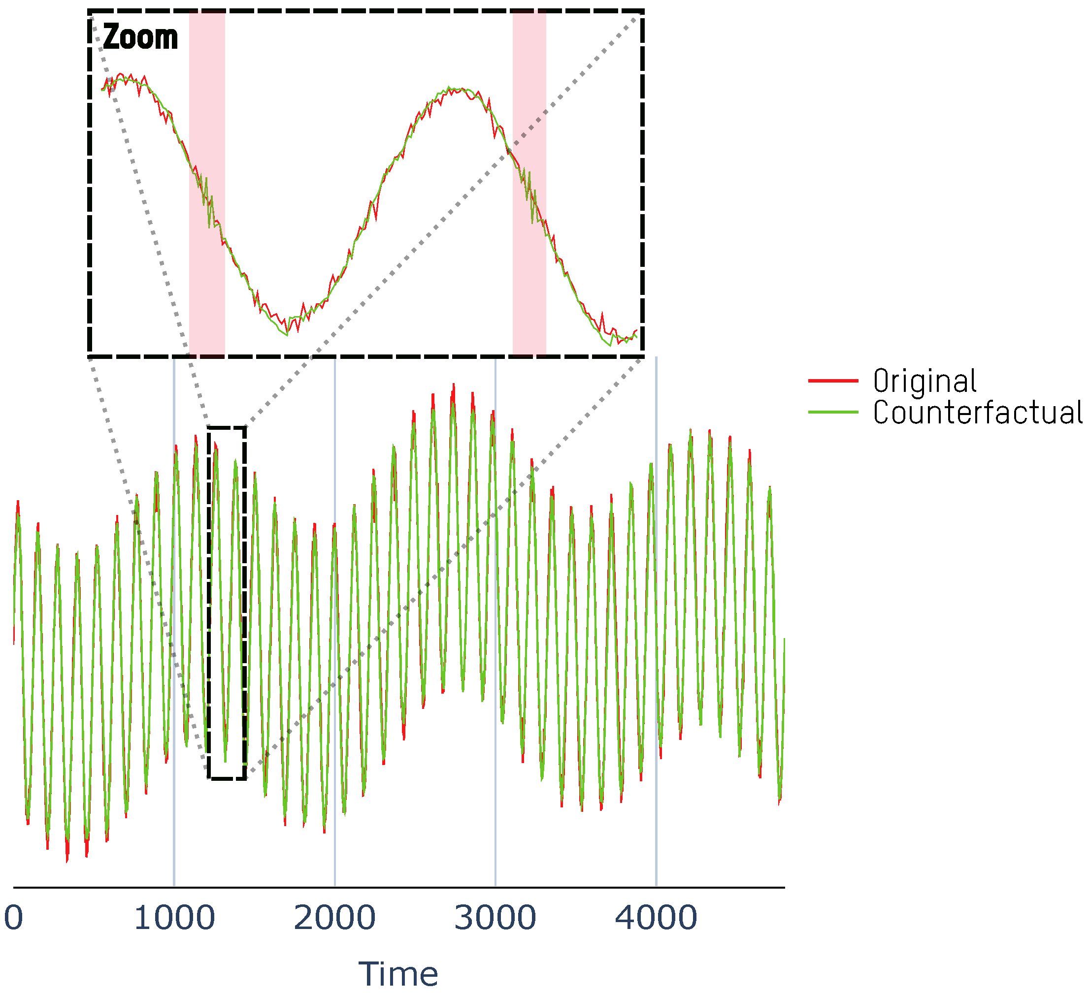
Figure 12 illustrates the utilization of RTGCEx for addressing anomalies. The input to the model is a simulation that contains anomalies caused by a crack in the inner race. These anomalies occur periodically as the bearing passes through the crack, and they are correctly identified by f ( · ) with a label of 1. In this scenario, RTGCEx can be employed to determine the minimal modifications necessary to the anomalous simulation for it to be classified as normal by f ( · ) . In the figure, the red signal represents the anomalous journey and the green signal represents the signal generated by RTGCEx. Upon closer examination, it can be observed that RTGCEx focuses on altering the areas where the anomalies appear, as indicated by the red shaded area.
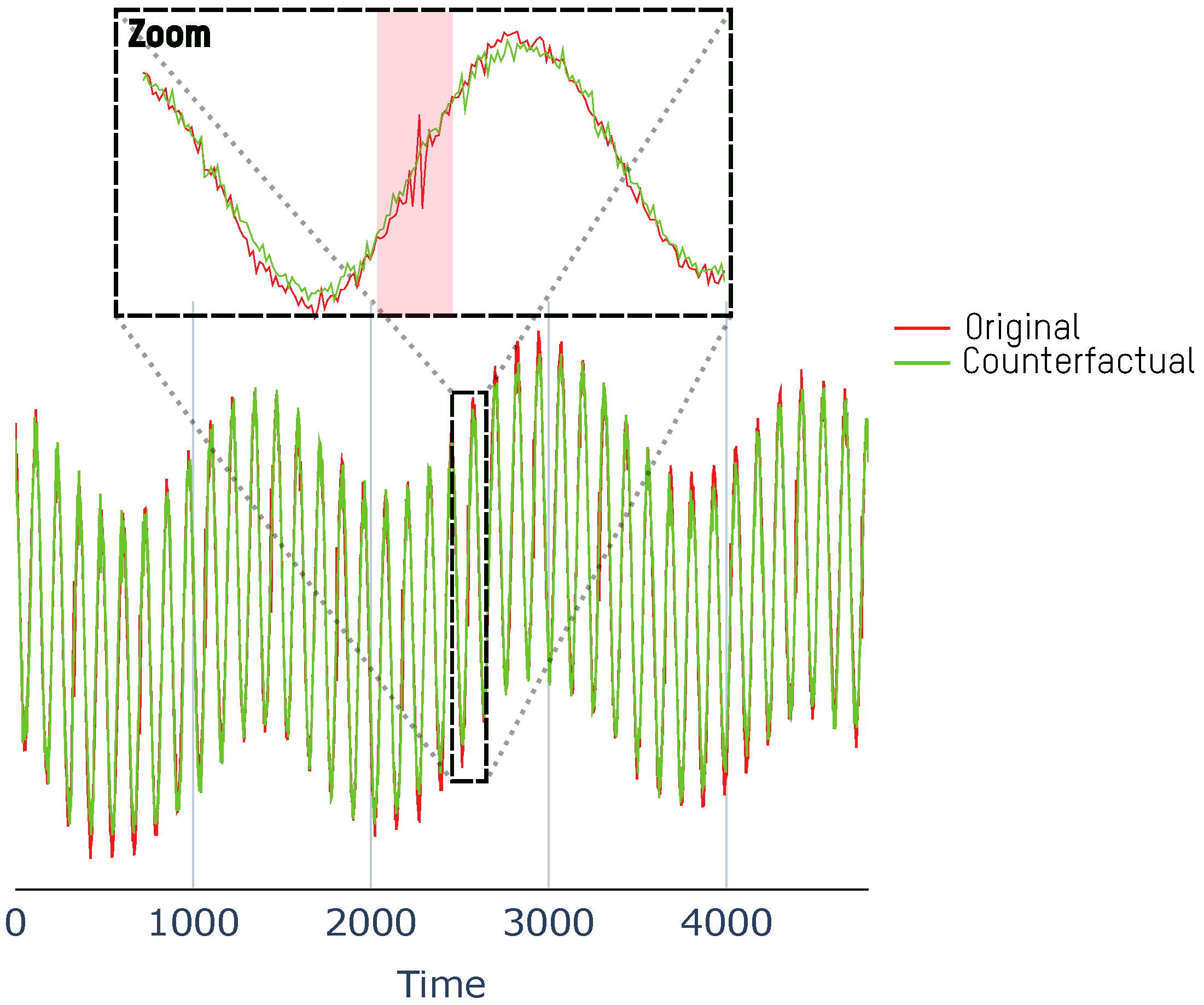
As previously mentioned, in addition to its use for identifying and rectifying anomalies, RTGCEx can also be utilized as a generator of anomalous data. Figure 13 provides an example of this application. The figure shows an input representing a non-anomalous journey of the gearbox, represented in red, and the changes that would need to be made, represented in green, to create an anomalous journey. It can be observed that RTGCEx has introduced several anomalies in the input data, highlighted by the red shaded areas, simulating the behavior that the accelerometer would have should cracks form in the inner race. This capability allows for the creation of anomalous data for understanding unusual behaviors or to create anomalous data in unbalanced scenarios, for example.
To measure the validity of the generated counterfactuals and the influence that each term of the loss function has on the final result, in Table 5, we measured the interpretability based on the three terms of the loss function of Equations (12), (14) and (15). In this table, each row corresponds to the results obtained according to which terms were used in the loss function, i.e.,
RTGCEx wo L AE : L = α · L G ( x , x c f ) + β · L D ( y c f , y c f ) RTGCEx wo L G : L = β · L f ( y c f , y c f ) + γ · L AE ( x c f , x c f ) RTGCEx : L = α · L G ( x , x c f ) + β · L f ( y c f , y c f ) + γ · L AE ( x c f , x c f )
This table presents the results of an evaluation of each term’s impact in the RTGCEx algorithm’s loss function on counterfactual generation. The results demonstrate that the term which ensures data similarity (represented by L G ) is crucial for generating counterfactual explanations that are highly similar to the input data and involve minimal changes. Removal of this term from the loss function leads to counterfactuals that are dissimilar to the input data and involve significant changes. The numerical analysis clearly shows this, as the closeness loss increases from 3.59 × 10 4 to 0.056 , and the data manifold loss increases from 1.29 × 10 4 to 2.32 × 10 4 upon removal of this term. Inclusion of this term in the loss function results in small values in data closeness loss, specifically 3.23 × 10 4 for RTGCEx without L AE and 3.59 × 10 4 for RTGCEx, indicating that the generated counterfactuals involve minor modifications to the input data. Furthermore, the value of the data manifold loss is low for RTGCEx and also when L AE is removed, indicating that the changes made are logical in both cases. The counterfactual loss is not significantly different across all methods, as the class of the counterfactual instances matches the intended class in all cases.
The amortized inference requirement is particularly important in anomaly detection [24], as a quick response is often required when an anomaly occurs. Therefore, the table also shows the average time it takes for the model to generate explanations for a single instance and for the entire test dataset (2020 instances). All methods take the same amount of time, as the generator used to generate the explanations has the same architecture in all three cases. For a single explanation, the generator takes on average 0.062 s with a variation of 0.091 s, while generating explanations for the whole test set takes 5.46 s. This demonstrates that the proposed method provides counterfactual explanations in real time, satisfying the amortized inference property.

6. Conclusions

In this study, we propose RTGCEx, a real-time, model-agnostic method for generating user-driven counterfactual explanations. The proposed method employs autoencoders trained with a multiobjective loss function to generate valid and data-close counterfactuals that align with the user’s desired outcome. The effectiveness of RTGCEx is demonstrated in different domains with different data types. Specifically, our results on the MNIST dataset show that RTGCEx outperforms classical methods in terms of both speed and efficacy, achieving lower IM2 values while maintaining similar IM1 values in significantly less time. We also observed that IM1 does not always accurately reflect the interpretability of the generated instances, as instances with lower values of IM1 were sometimes less realistic. Additionally, the results of our tests on the Gearbox dataset demonstrate that RTGCEx is effective for identifying and rectifying anomalies, achieving low values in all terms of the loss function and satisfying the desired properties.

Author Contributions

Conceptualization, J.L.S.; methodology, J.L.S., X.D.C.G. and E.Z.U.; software, J.L.S.; validation, J.L.S.; formal analysis, J.L.S.; investigation, J.L.S.; resources, J.L.S.; data curation, J.L.S.; writing—original draft preparation, J.L.S.; writing—review and editing, X.D.C.G. and E.Z.U.; visualization, J.L.S.; supervision, X.D.C.G. and E.Z.U.; project administration, X.D.C.G. and E.Z.U.; funding acquisition, J.L.S., X.D.C.G. and E.Z.U. All authors have read and agreed to the published version of the manuscript.

Funding

This research was funded by DREMIND project of the Basque Government under Grant KK-2022/00049 from the ELKARTEK program.

Institutional Review Board Statement

Not applicable.

Informed Consent Statement

Not applicable.

Data Availability Statement

The Gearbox data can be obtained using this simulator: https://www.mathworks.com/help/signal/examples/vibration-analysis-of-rotating-machinery.html (accessed on 1 February 2023).

Acknowledgments

Jokin Labaien, Xabier De Carlos and Ekhi Zugasti are supported by the DREMIND project of the Basque Government under Grant KK-2022/00049 from the ELKARTEK program. Ekhi Zugasti is part of the Intelligent Systems for Industrial Systems research group of Mondragon Unibertsitatea (IT1676-22), supported by the Department of Education, Universities and Research of the Basque Country. Jokin Labaien, Xabier De Carlos and Ekhi Zugasti are part of the “Intelligent Digital Platforms” IBAT collaboration team between Ikerlan and Mondragon Goi Eskola Politeknikoa.

Conflicts of Interest

The authors declare no conflict of interest.

References

  1. Ribeiro, M.T.; Singh, S.; Guestrin, C. Anchors: High-precision model-agnostic explanations. In Proceedings of the Thirty-Second AAAI Conference on Artificial Intelligence, New Orleans, LA, USA, 2–7 February 2018. [Google Scholar]
  2. Friedman, J.H.; Popescu, B.E. Predictive learning via rule ensembles. Ann. Appl. Stat. 2008, 2, 916–954. [Google Scholar] [CrossRef]
  3. Lundberg, S.M.; Lee, S.I. A unified approach to interpreting model predictions. In Proceedings of the Advances in Neural Information Processing Systems, Long Beach, CA, USA, 4–9 December 2017; pp. 4765–4774. [Google Scholar]
  4. Ribeiro, M.T.; Singh, S.; Guestrin, C. Why should i trust you? Explaining the predictions of any classifier. In Proceedings of the 22nd ACM CA, International Conference on Knowledge Discovery and Data Mining, San Francisco, CA, USA, 13–17 August 2016; pp. 1135–1144. [Google Scholar]
  5. Sundararajan, M.; Taly, A.; Yan, Q. Axiomatic attribution for deep networks. In Proceedings of the 34th International Conference on Machine Learning, Sydney, Australia, 6–11 August 2017; Volume 70, pp. 3319–3328. [Google Scholar]
  6. Stepin, I.; Alonso, J.M.; Catala, A.; Pereira-Fariña, M. A Survey of Contrastive and Counterfactual Explanation Generation Methods for Explainable Artificial Intelligence. IEEE Access 2021, 9, 11974–12001. [Google Scholar] [CrossRef]
  7. Verma, S.; Dickerson, J.; Hines, K. Counterfactual Explanations for Machine Learning: A Review. arXiv 2020, arXiv:2010.10596. [Google Scholar]
  8. Artelt, A.; Hammer, B. On the computation of counterfactual explanations—A survey. arXiv 2019, arXiv:1911.07749. [Google Scholar]
  9. Dhurandhar, A.; Chen, P.Y.; Luss, R.; Tu, C.C.; Ting, P.; Shanmugam, K.; Das, P. Explanations based on the missing: Towards contrastive explanations with pertinent negatives. In Proceedings of the Advances in Neural Information Processing Systems, Montreal, QC, Canada, 3–8 December 2018; pp. 592–603. [Google Scholar]
  10. Van Looveren, A.; Klaise, J. Interpretable counterfactual explanations guided by prototypes. arXiv 2019, arXiv:1907.02584. [Google Scholar]
  11. Kenny, E.M.; Keane, M.T. On generating plausible counterfactual and semi-factual explanations for deep learning. arXiv 2020, arXiv:2009.06399. [Google Scholar] [CrossRef]
  12. Nugent, C.; Doyle, D.; Cunningham, P. Gaining insight through case-based explanation. J. Intell. Inf. Syst. 2009, 32, 267–295. [Google Scholar] [CrossRef] [Green Version]
  13. Mothilal, R.K.; Sharma, A.; Tan, C. Explaining machine learning classifiers through diverse counterfactual explanations. In Proceedings of the 2020 Conference on Fairness, Accountability, and Transparency, Barcelona, Spain, 27–30 January 2020; pp. 607–617. [Google Scholar]
  14. Nemirovsky, D.; Thiebaut, N.; Xu, Y.; Gupta, A. CounteRGAN: Generating Realistic Counterfactuals with Residual Generative Adversarial Nets. arXiv 2020, arXiv:2009.05199. [Google Scholar]
  15. Liu, S.; Kailkhura, B.; Loveland, D.; Han, Y. Generative counterfactual introspection for explainable deep learning. arXiv 2019, arXiv:1907.03077. [Google Scholar]
  16. Mahajan, D.; Tan, C.; Sharma, A. Preserving causal constraints in counterfactual explanations for machine learning classifiers. arXiv 2019, arXiv:1912.03277. [Google Scholar]
  17. Saxena, D.; Cao, J. Generative Adversarial Networks (GANs) Challenges, Solutions, and Future Directions. ACM Comput. Surv. 2021, 54, 1–42. [Google Scholar] [CrossRef]
  18. Balasubramanian, R.; Sharpe, S.; Barr, B.; Wittenbach, J.; Bruss, C.B. Latent-CF: A Simple Baseline for Reverse Counterfactual Explanations. arXiv 2020, arXiv:2012.09301. [Google Scholar]
  19. LeCun, Y.; Bottou, L.; Bengio, Y.; Haffner, P. Gradient-based learning applied to document recognition. Proc. IEEE 1998, 86, 2278–2324. [Google Scholar] [CrossRef] [Green Version]
  20. Mathworks Gearbox Simulator. Available online: https://www.mathworks.com/help/signal/examples/vibration-analysis-of-rotating-machinery.html (accessed on 1 February 2023).
  21. Canizo, M.; Triguero, I.; Conde, A.; Onieva, E. Multi-head CNN–RNN for multi-time series anomaly detection: An industrial case study. Neurocomputing 2019, 363, 246–260. [Google Scholar] [CrossRef]
  22. Lin, M.; Lucas, H.C., Jr.; Shmueli, G. Research commentary—Too big to fail: Large samples and the p-value problem. Inf. Syst. Res. 2013, 24, 906–917. [Google Scholar] [CrossRef] [Green Version]
  23. Hvilshøj, F.; Iosifidis, A.; Assent, I. On quantitative evaluations of counterfactuals. arXiv 2021, arXiv:2111.00177. [Google Scholar]
  24. Schemmer, M.; Holstein, J.; Bauer, N.; Kühl, N.; Satzger, G. Towards Meaningful Anomaly Detection: The Effect of Counterfactual Explanations on the Investigation of Anomalies in Multivariate Time Series. arXiv 2023, arXiv:2302.03302. [Google Scholar]
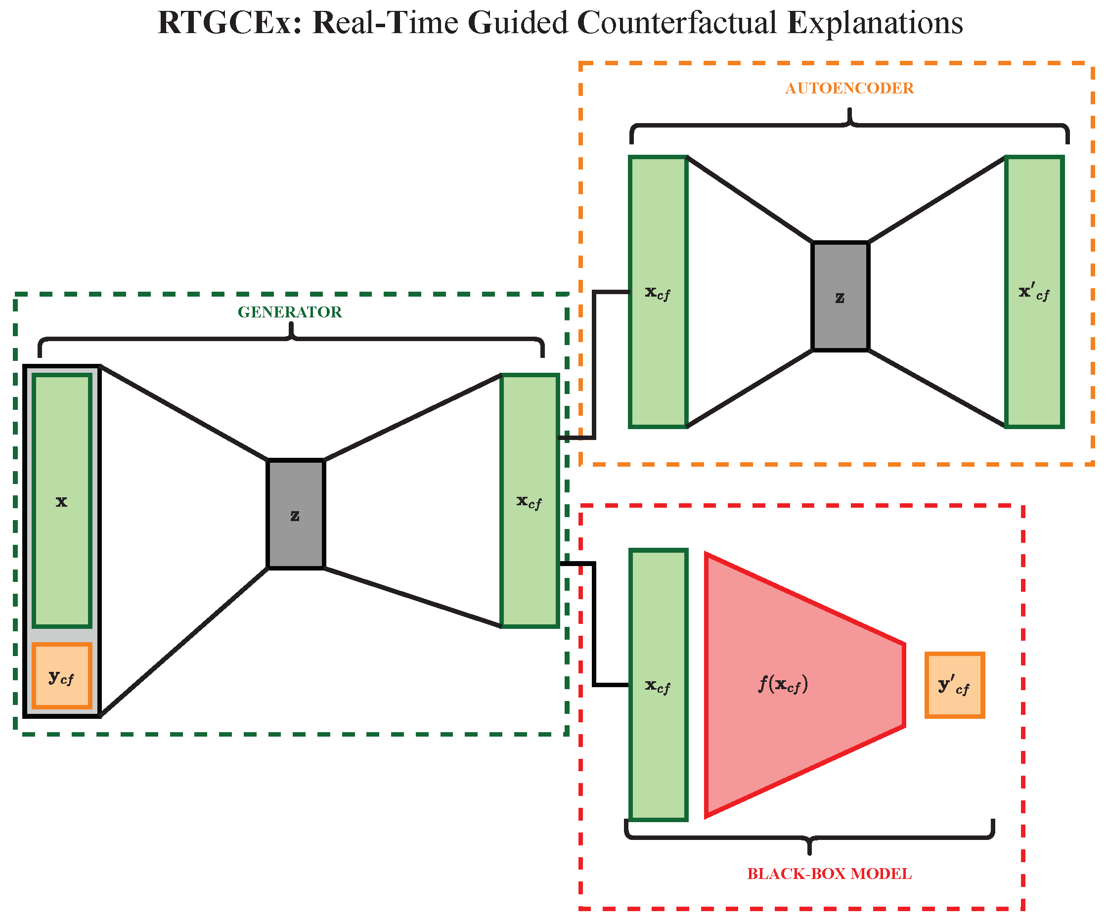
Figure 1. Real-Time Guided Counterfactual Explanations.
Applsci 13 02912 g001
Figure 2. General scheme of the gearbox.
Applsci 13 02912 g002
Figure 3. Inner race affected by a crack.
Applsci 13 02912 g003
Figure 4. Black-box model f ( · ) used in MNIST.
Applsci 13 02912 g004
Figure 5. AE used for ensuring data-manifold closeness.
Applsci 13 02912 g005
Figure 6. Proposed black-box model.
Applsci 13 02912 g006
Figure 7. Composition of the convolutional blocks of the CNN backbone.
Applsci 13 02912 g007
Figure 8. Proposed generator.
Applsci 13 02912 g008
Figure 9. Examples of original and counterfactual instances generated with CFPROTO, RTGCEx without AE, and RTGCEx.
Applsci 13 02912 g009
Figure 10. Distribution plots for each method in terms of IM1 and IM2 (×10) metrics. The dashed lines represent the mean. (a) IM1 distribution plots. (b) IM2 (×10) distribution plots.
Applsci 13 02912 g010
Figure 11. Examples of two counterfactual instances generated by CFPROTO and RTGCEx, where IM2 is lower when using RTGCEx, and IM1 is higher.
Applsci 13 02912 g011
Figure 12. An anomalous sample and the counterfactual explanation for showing normal behavior.
Applsci 13 02912 g012
Figure 13. A normal sample and the counterfactual explanation for introducing anomalies.
Applsci 13 02912 g013
Table 1. Results obtained for the AE in terms of MSE and for the black-box model in terms of accuracy.
ModelAEBlack-Box Model
MetricMSEAccuracy
Value0.0070.991
Table 2. Summary of the results obtained in test for each method. Best results are highlighted in bold.
MethodIM1IM2 (×10)Speed (s/it)
MeanIQRMeanIQRMeanIQR
CFPROTO1.200.391.200.8317.400.09
RTGCEx wo AE1.400.631.120.740.140.01
RTGCEx1.210.580.910.630.140.01
Table 3. This table represents the probabilities that a counterfactual instance has a lower IM1 or IM2 depending on the method used.
MethodCFPROTORTGCEx wo AERTGCEx
IM1IM2IM1IM2IM1IM2
CFPROTO-0.660.530.500.38
RTGCEx wo AE0.340.47-0.260.24
RTGCEx0.500.620.740.76-
Table 4. Results obtained with the autoencoder and the black-box model f ( · ) .
ModelAEBlack-Box Model
MetricMSEPRF1
Value 2.301 × 10 4 0.97310.986
Table 5. Mean values obtained for each loss function in test data using the three variations of the losses optimized in RTGCEx.
MethodCloseness LossCounterfactual LossData Manifold LossSpeed (s)
One SampleTest Data
RTGCEx wo L AE 3.23 × 10 4 4.91 × 10 7 1.60 × 10 4 0.062 ± 0.091 5.46
RTGCEx wo L G 0.056 4.18 × 10 7 2.32 × 10 4
RTGCEx 3.59 × 10 4 5.83 × 10 7 1.29 × 10 4
Disclaimer/Publisher’s Note: The statements, opinions and data contained in all publications are solely those of the individual author(s) and contributor(s) and not of MDPI and/or the editor(s). MDPI and/or the editor(s) disclaim responsibility for any injury to people or property resulting from any ideas, methods, instructions or products referred to in the content.