A Hybrid Deep Learning Model for Multi-Station Classification and Passenger Flow Prediction

Abstract

Multiple station passenger flow prediction is crucial but challenging for intelligent transportation systems. Recently, deep learning models have been widely applied in multi-station passenger flow prediction. However, flows at the same station in different periods, or different stations in the same period, always present different characteristics. These indicate that globally extracting spatio-temporal features for multi-station passenger flow prediction may only be powerful enough to achieve the excepted performance for some stations. Therefore, a novel two-step multi-station passenger flow prediction model is proposed. First, an unsupervised clustering method for station classification using pure passenger flow is proposed based on the Transformer encoder and K-Means. Two novel evaluation metrics are introduced to verify the effectiveness of the classification results. Then, based on the classification results, a passenger flow prediction model is proposed for every type of station. Residual network (ResNet) and graph convolution network (GCN) are applied for spatial feature extraction, and attention long short-term memory network (AttLSTM) is used for temporal feature extraction. Integrating results for every type of station creates a prediction model for all stations in the network. Experiments are conducted on two real-world ridership datasets. The proposed model performs better than unclassified results in multi-station passenger flow prediction.

1. Introduction

With the rapid development of urban public transportation (UPT), passenger flow prediction is very significant in meeting passengers’ travel needs, which is one of the important issues in improving the UPT services.

Recently, the research on passenger flow prediction has been converted from a single station to multiple stations because multi-station passenger flow prediction is more applicable in UPT. Due to the complex spatial features and time-varying traffic patterns of networks [1], passenger flow at a single station has been simultaneously affected by the spatio-temporal features of historical passenger flow at the directly or indirectly connected stations in the whole network [2]. Thus, a single station passenger flow prediction model could not dynamically and effectively predict the spatio-temporal distribution and congestion in the entire network, which limits the real-time passenger flow organization, formulation, and adjustment of the operation management strategy [3]. To this end, more and more researchers have devoted themselves to passenger flow prediction for multiple stations. How to deeply capture the complex spatio-temporal features to make a more accurate passenger flow prediction model for the whole network stations is becoming a hotspot in recent studies.

In addition, many well-performing deep learning models continue to emerge, focusing on capturing spatio-temporal correlation between stations by constructing spatio-temporal feature learners (STFL) in traffic inflow and outflow prediction [4]. Bogaerts et al. [5] proposed a deep neural network that simultaneously extracted the spatial features using graph convolution neural network (GCN) and the temporal features using long short-term memory (LSTM) to make both short-term and long-term traffic flow predictions. Li et al. [6] proposed a deep learning model combining convolutional LSTM (ConvLSTM) and stack autoencoder (SAE) to predict the short-term passenger flow of URT for multiple stations. ConvLSTM was used to extract spatio-temporal features of passenger flow based on thirteen external factors related to passenger flow. Zhang et al. [7] proposed a deep learning-based model named GCN-Transformer, which comprised the GCN for spatial features extracting and the modified Transformer for temporal features extracting for short-term passenger flow prediction of multiple stations.

The above models are all hybrid models which capture the spatio-temporal features simultaneously to predict passenger flow at stations in the whole network. However, the passenger flow at the same station in different periods presents different characteristics, and various stations in the same period also have different passenger flow changes. We illustrate the differences by using Figure 1 as an example.

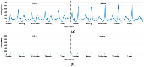
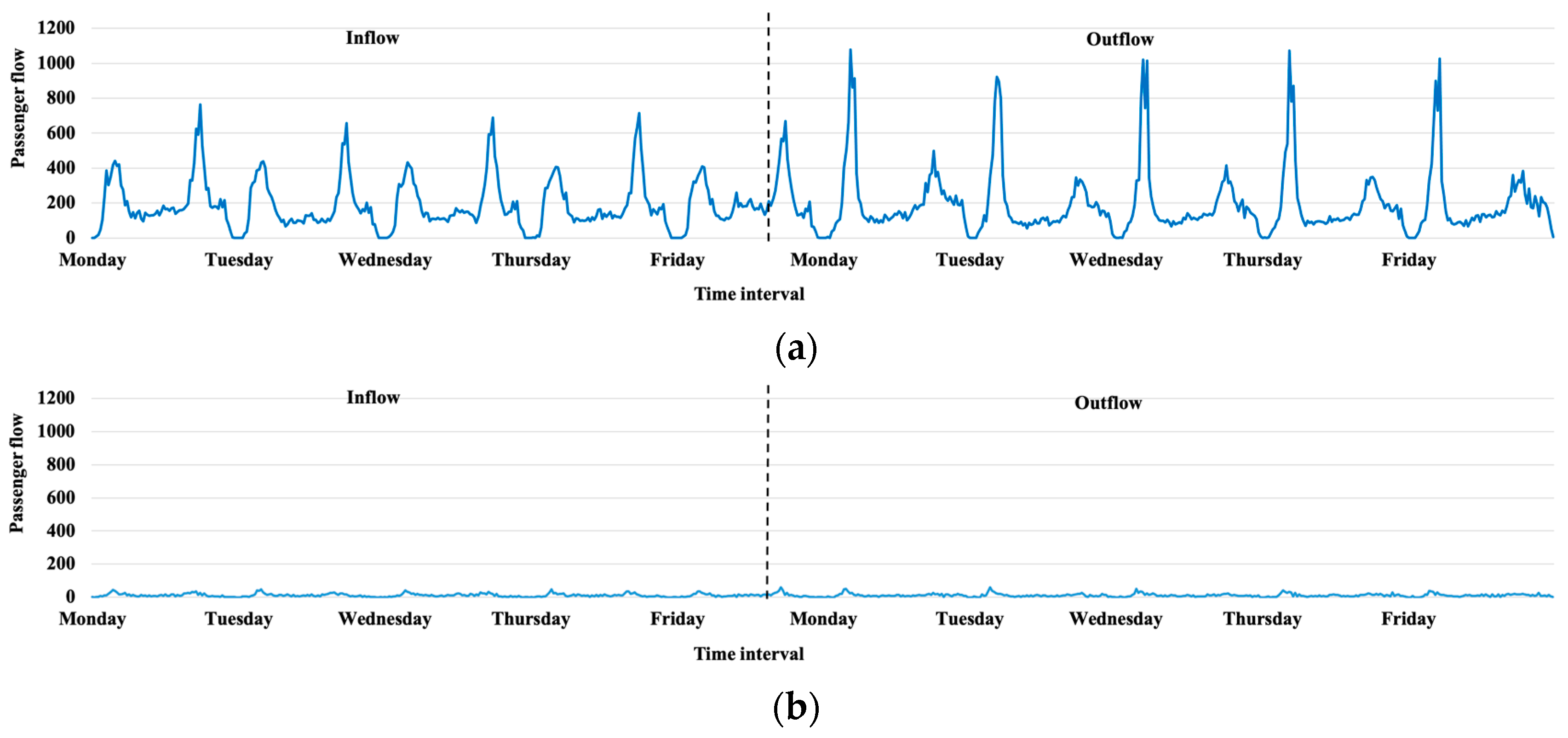
Figure 1. Inflow and outflow at the two stations in the Xiamen BRT. (a) Xianhou Station; (b) Dongzhai Station.

Figure 1a,b show one-week inbound and outbound passenger flow from 4 March 2019 to 8 March 2019 at Xianhou Station and Dongzhai Station in the Xiamen bus rapid transit (BRT), respectively. Both stations had clear characteristics of inbound and outbound tidal flows in their respective time intervals, but the difference was that the largest volume of inflow and outflow between the two stations was nearly 16 times in the same period. Their variability was also quite different.

These indicate that globally extracting the spatio-temporal features for multi-station passenger flow prediction in the whole network may not be powerful enough to achieve the expected performance for every station [8]. Making a more accurate multiple-station passenger flow prediction model for every station is necessary and significant.

Furthermore, most existing studies on urban metro station classification were mainly based on the features of land location [9], point of interest (POI) [10,11,12], population distribution [11], station location [11,13], length of road network [11], passenger flow [9,11,12,14,15], and their combinations. These studies were mainly divided into two directions [16]. The first was “place oriented,” which focused on land use function. And the other was “station oriented,” which focused on station function. To our best knowledge, passenger flow is used as one of the factors in many existing studies for station classification, not as the only factor. There needs to be a study that uses passenger flow as the only feature for multi-station classification based on the similarities of passenger flow among stations. Thus, the existing research on station classification was much more applicable for urban planning and station layout planning, rather than for passenger flow prediction. Furthermore, the previous studies preferred to visualize the passenger flow in the same type of station [9,11,13,14] to verify the effectiveness of station classification, which were not objectivity.

Considering the historical passenger flow is the most important influence factor in passenger flow prediction. Some scholars have classified passenger flow in different time intervals for passenger flow prediction. For example, Wang et. al [17] designed an adaptive K-Means to cluster the time intervals with similar passenger flow at Shenzhen North Railway Station. Passenger flow belonging to the same category had the same time interval tag. Then, this tag combined with the historical passenger flow was used in the passenger flow prediction task. Tan et al. [18] used K-Means to divide the 10-month passenger flow into 16 categories, and then built 16 sub-prediction models at Chengdu East Railway Station. Although the above studies have classified passenger flow classification to further improve the accuracy of passenger flow prediction, they are only for a single station.

To sum up, there are few studies that applying station classification on multi-station passenger flow prediction. Inspired by the fact that the same types of stations have more similar passenger flow, classifying the stations based on the pure passenger flow and then predicting the passenger flow for every type of station with similar flows may be a more effective strategy to improve the prediction accuracy; therefore, we have proposed a novel multi-station passenger flow prediction model that consists of a Transformer encoder, K-Means, Residual Network (ResNet), graph convolution network (GCN), and attention long short-term memory ((Transformer-K-Means)-(ResNet-GCN-AttLSTM)), which can better extract the spatio-temporal features for the same types of stations with similar flows in the whole network. This model uses a two-step strategy: classification and prediction, to achieve a better performance for multi-station passenger flow prediction. To our best knowledge, this is the first time to apply station classification before the downstream task of passenger flow prediction. The main contributions of this paper are summarized as follows:

(1) We propose a novel unsupervised clustering method for station classification using pure passenger flow data. First, this method applies a Transformer encoder to extract the spatio-temporal features from the inflow and outflow data, and then it applies the extracted spatio-temporal features to K-Means for station classification.

(2) Quantitatively, two novel evaluation metrics have been introduced to verify the effectiveness of the results of station classification.

(3) Based on the results of station classification, a deep spatio-temporal network framework, ResNet-GCN-AttLSTM, for passenger flow prediction at each type of station has been proposed. By integrating the passenger flow prediction results of every type of station, a novel passenger flow prediction model for all stations in the whole network is constructed. We implement the proposed model on two real-world ridership datasets to demonstrate its performance.

The remainder of the paper is organized as follows. Section 2 provides the proposed methodology in detail. In Section 3, two real-world ridership datasets in the Beijing metro and the Xiamen BRT are presented. The performances in station classification and passenger flow prediction for multiple stations are provided extensively. Finally, conclusions are drawn and future research directions are indicated in Section 4.

2. Methodology

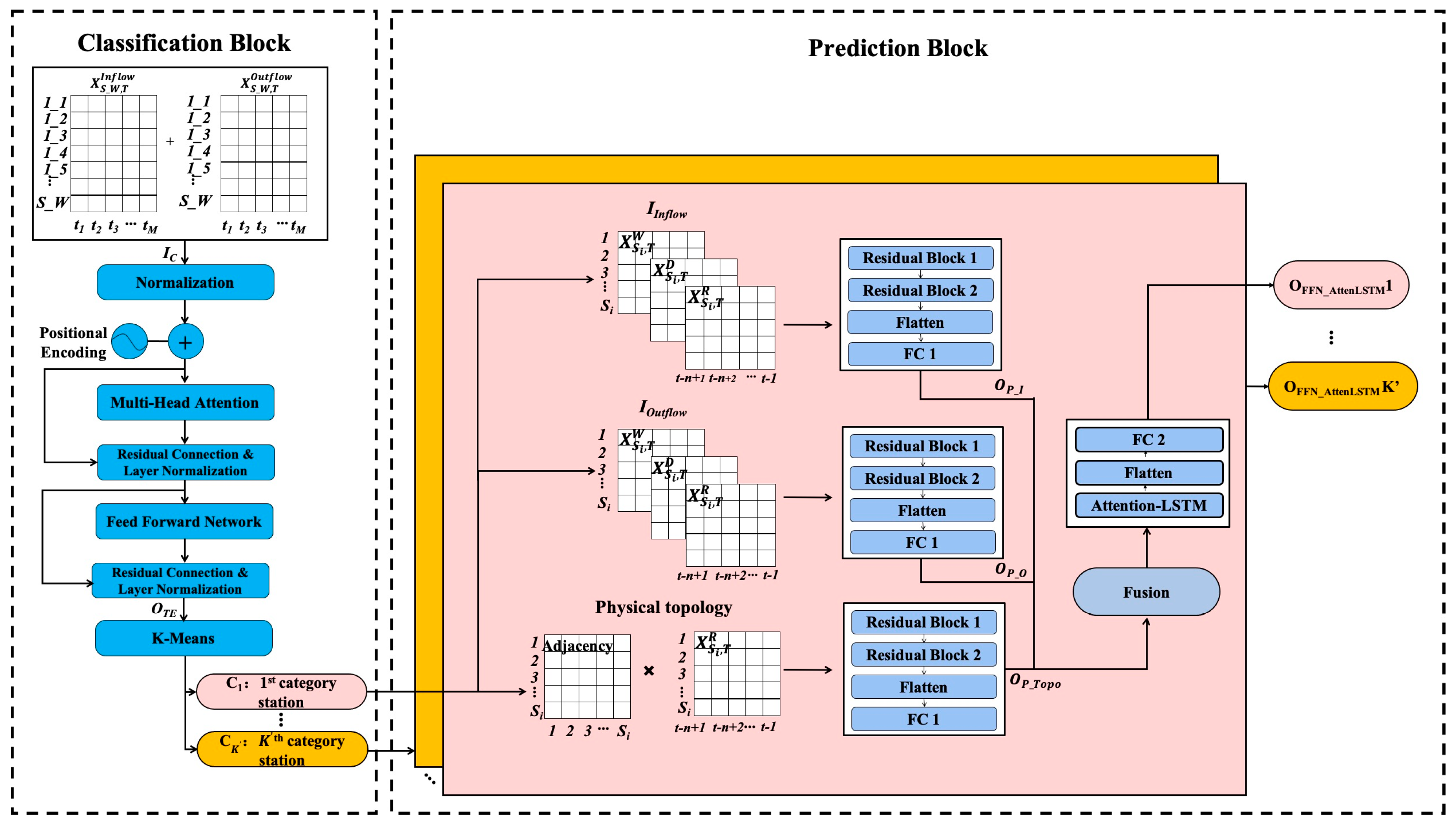
In this section, we introduce the detailed steps for the construction and combination of the proposed model ((Transformer-K-Means)-(ResNet-GCN-AttLSTM)). As shown in Figure 2, it consists of two blocks: the classification block and the prediction block. The classification block extracts the deep features from the inflow and outflow data based on the Transformer encoder, then classifies the stations based on K-Means. A prediction block is used to predict the inflow for each type of station, and then integrate them as the final result for all stations in the whole network.

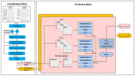
Figure 2. The framework of the proposed (Transformer-K-Means)-(ResNet-GCN-AttLSTM).

As shown in Figure 1, the inflow and outflow at the different stations, even at the same station, are very different. Inflow prediction is more significant for avoiding congestion among stations. Thus, we use both the inflow and outflow data in the classification block to predict the inflow in the prediction block.

2.1. Classification Block

A classification block is used to classify all the stations into several categories in the whole network. Transformer Encoder is used for feature extraction from the inflow and outflow data, and then the extracted feature based on Transformer Encoder will be sent to K-Means for station classification.

2.1.1. Transformer Encoder

The Transformer is wholly based on the attention mechanism, which can simultaneously obtain global and weighted information. Moreover, its multi-head mechanism can map input features from different perspectives. Undoubtedly, its expression ability becomes stronger, which is able to better extract the deep features for time-series problems [16]. Inspired by its powerful ability, we apply Transformer for feature extraction to achieve better clustering results for station classification with the pure passenger flow data in this paper. Furthermore, Transformer is mainly composed of an encoder and a decoder. Our research focuses on the task of passenger flow feature extraction rather than natural language processing (NLP) tasks, so we only use the encoder.

To ensure the effectiveness of station classification, we use more than one week of inflow and outflow data as the inputs. As shown in Figure 2, the inflow and outflow data will be sent into the Transformer encoder, which can be expressed as a matrix $X_{S\_W,T}^P$ shown in Equation (1).

$$X_{S\_W,T}^P=\left\{\begin{array}{ccc}\begin{array}{cc}{x}_{1\_1, t_1}^P& x_{1\_1, t_2}^P\\ x_{1\_2, t_1}^P& x_{1\_2, t_2}^P\end{array}& \cdots & \begin{array}{c}{x}_{1\_1, t_M}^P\\ x_{1\_2, t_M}^P\end{array}\\ \begin{array}{cc}⋮ & ⋮\end{array}& \ddots & ⋮\\ \begin{array}{cc}{x}_{S\_W, t_1}^P& x_{S\_W, t_2}^P\end{array}& \cdots & x_{S\_W, t_M}^P\end{array}\right\}$$

(1)

$$I_C=X_{S\_W,T}^{Inflow}\left|\right|X_{S\_W,T}^{Outflow}$$

(2)

where S is the number of stations in the whole network, W is the number of weeks, and M = $DS\times days$ is the number of time intervals during a week. Daily sample data (DS) are the number of time intervals per day; days are the number of days during a week. T = {t₁, t₂,…, t_M} is a series of time intervals in a week.$P\in${Inflow, Outflow} refers to the inflow or outflow patterns. $X_{S\_W,T}^{Inflow}\in {ℝ}^{\left(S\times W\right)\times \left(DS\times days\right)}$, $X_{S\_W,T}^{Outflow}\in {ℝ}^{\left(S\times W\right)\times \left(DS\times days\right)}$ represent the inflow data and outflow data, respectively. Inflow and outflow data will be concatenated by column, which is the inputs in the Transformer encoder ($I_C\in {ℝ}^{\left(S\times W\right)\times \left(2\times DS\times days\right)}$) shown in Equation (2).

(1)

Normalization

First, $I_C$ is standardized as ${(I_C)}_{SD}$ based on Equation (3).

$${(I_C)}_{SD}=\frac{I_C-{(I_C)}_{mean}}{{(I_C)}_{std}}$$

(3)

where ${(I_C)}_{mean}$ is the mean value of $I_C$; ${(I_C)}_{std}$ is the standard deviation of $I_C$. ${(I_C)}_{SD}\in {ℝ}^{\left(S\times W\right)\times \left(2\times DS\times days\right)}$ with two dimensions will be transformed to ${(I_C)}_{SD\_Day}\in {ℝ}^{\left(S\times W\right)\times days\times \left(2\times DS\right)}$ and ${(I_C)}_{SD\_Interval}\in {ℝ}^{\left(S\times W\right)\times DS\times \left(2\times days\right)}$ with three dimensions, respectively.

(2)

Positional Encoding

After that, we follow the positional encoding in the original Transformer model [16] to realize the position encoding of ${(I_C)}_{SD\_Day}$ and ${(I_C)}_{SD\_Interval}$ as $PE\left({(I_C)}_{SD\_Day}\right)$ and $PE\left({(I_C)}_{SD\_Interval}\right)$ based on Equations (4) and (5), respectively.

$$P{E}_{(pos,2i)}=sin(\frac{pos}{{10000}^{\frac{2i}{d_{model}}}}) (i\in (0, 1/d_{\mathit{model}}, \mathit{pos}\in (1,S\times W))$$

(4)

$$P{E}_{\left(pos,2i+1\right)}=cos(\frac{pos}{{10000}^{\frac{2i}{d_{model}}}}) (i\in (0, 1/d_{\mathit{model}}, \mathit{pos}\in (1,S\times W))$$

(5)

where $d_{model}$ in Equations (4) and (5) is set as $2\times DS$, $2\times days$ in ${(I_C)}_{SD\_Day}$ and ${(I_C)}_{SD\_Interval}$, respectively. $PE\left({(I_C)}_{SD\_Day}\right)\in {ℝ}^{\left(S\times W\right)\times d_{model}}\left(d_{model}=2\times DS\right)$, and $PE\left({(I_C)}_{SD\_Interval}\right)\in {ℝ}^{\left(S\times W\right)\times d_{model}}\left(d_{model}=2\times days\right)$ are two dimensions, respectively.

(3)

Multi-head Attention

$\mathrm{Take}PE\left({(I_C)}_{SD\_Day}\right)\mathrm{for}\mathrm{example},PE\left({(I_C)}_{SD\_Interval}\right)$ has the same processing.

$PE\left({(I_C)}_{SD\_Day}\right)$ and $PE\left({(I_C)}_{SD\_Interval}\right)$ will be transformed to Qⁱ, Kⁱ, and Vⁱ based on Equations (6)–(8), respectively. We use a particular attention called “Scaled Dot-Product Attention” [16]. The input consists of Qⁱ and Kⁱ with both dimensions $d_k$ and Vⁱ with dimension $d_v$. The term $d_v$ is the dimension of output. Then, Qⁱ, Kⁱ, and Vⁱ will be input into the multi-head attention layer to calculate the attention scores ($hea{d}_i)$ based on Equation (9) for every head. By concatenating the $hea{d}_i$ by column, $I_{att\_Day}$ and $I_{att\_Interval}$ will be obtained as the outputs based on Equation (10), respectively.

$$Q^i=PE\left({(I_C)}_{SD\_Day}\right)\times {W_q}^i$$

(6)

$$K^i=PE\left({(I_C)}_{SD\_Day}\right)\times {W_k}^i$$

(7)

$$V^i=PE\left({(I_C)}_{SD\_Day}\right)\times {W_v}^i$$

(8)

$$hea{d}_i={{\displaystyle \sum }}_{\mathrm{i}}^N\mathrm{Attention}\left(Q^i,K^i,V^i\right)=\mathrm{softmax}\left(\frac{Q^i{\left(K^i\right)}^T}{\sqrt{d_{K^i}}}\right)V^i$$

(9)

$$I_{att\_Day}=\left(hea{d}_1\left|\left| hea{d}_2,\dots , \right|\right|hea{d}_N\right)W_o$$

(10)

where W_qⁱ$\in {ℝ}^{d_{model}\times d_k}$, W_kⁱ$\in {ℝ}^{d_{model}\times d_k}$, W_vⁱ$\in {ℝ}^{d_{model}\times d_v}$, and $W_o\in {ℝ}^{\left(h\times d_v\right)\times d_{model}}$ are the trainable weights. The terms $d_k,$ and $d_v$ are the dimensions of Kⁱ and Vⁱ, respectively. N represents the number of heads, $i\in \left[1,N\right]$. $I_{att\_Day}\in {ℝ}^{\left(S\times W\right)\times \left(2\times DS\right)}$ and $I_{att\_Interval}\in {ℝ}^{\left(S\times W\right)\times \left(2\times days\right)}$ are the outputs of multi-head attention.

(4)

Residual Connection and Layer Normalization

$I_{att\_Day}$ and $I_{att\_Interval}$ will be sent to a residual connection [19] as $O_{att\_Day}$ and $O_{att\_Interval}$ based on Equations (11) and (12), respectively, and then followed by layer normalization as ${\left(O_{att\_Day}\right)}_{SD}$ and ${(O_{att\_Interval})}_{SD}$ based on Equation (3), respectively.

$$O_{att\_Day}=I_{att\_Day}+PE\left({(I_C)}_{SD\_Day}\right)$$

(11)

$$O_{att\_Interval}=I_{att\_Interval}+PE\left({(I_C)}_{SD\_Interval}\right)$$

(12)

(5)

Feed-Forward Network

${\left(O_{att\_Day}\right)}_{SD}$ and ${(O_{att\_Interval})}_{SD}$ will be sent to two feed-forward networks for full connection for further feature extraction based on Equations (13) and (14), respectively.

$$O_{FFN\_Day}=f_2(f_1({\left(O_{att\_Day}\right)}_{SD}\times W_1+b_1)\times W_2+b_2)$$

(13)

$$O_{FFN\_Interval}=f_2(f_1({\left(O_{att\_Interval}\right)}_{SD}\times W_1{}^{\prime }+b_1{}^{\prime })\times W_2{}^{\prime }+b_2{}^{\prime })$$

(14)

where $W_1$, $W_1{}^{\prime }$, $W_2$ and $W_2{}^{\prime }$ are the trainable weights, and $b_1$, $b_1{}^{\prime }$, $b_2$ and $b_2{}^{\prime }$ are the trainable biases.

(6)

The Output of the Transformer Encoder

$O_{FFN\_Day}$ and $O_{FFN\_Interval}$ will be sent for residual connection and layer normalization again as ${\left(O_{FFN\_Day}\right)}_{SD}{}^{\prime }\in {ℝ}^{\left(S\times W\right)\times \left(2\times days\right)}$ and ${\left(O_{FFN\_Interval}\right)}_{SD}{}^{\prime }\in {ℝ}^{\left(S\times W\right)\times \left(2\times DS\right)}$ based on Equations (3), (11) and (12), respectively. ${\left(O_{FFN\_Day}\right)}_{SD}{}^{\prime }$ and ${\left(O_{FFN\_Interval}\right)}_{SD}{}^{\prime }$ will be concatenated by column as $O_{TE}$ shown in Equation (15). $O_{TE}\in {ℝ}^{\left(S\times W\right)\times \left(2\times days+2\times DS\right)}$ is the final output in the Transformer encoder, which is the input sent into K-Means.

$$O_{TE}={\left(O_{FFN\_Day}\right)}_{SD}{}^{\prime }\left|\right|{\left(O_{FFN\_Interval}\right)}_{SD}{}^{\prime }$$

(15)

2.1.2. K-Means

K-Means is one of the most famous clustering algorithms, and is extensively used in unsupervised clustering tasks [11]. The key problem in K-Means is how to determine the value of K. K is the number of clusters, which is also the number of station categories in this paper.

Previous studies set K artificially [11], or used the elbow method [18]. To better determine K effectively, two novel evaluation metrics named same category rate (SCR) and average same category rate (ASCR) have been proposed. The ridership data used in our model are more than one week, and different weekly passenger flow at the same station may be similar. The clustering result is better if the same station of passenger flow in different weekly periods can be clustered into the same category. Inspired by this hypothesis, SCR and ASCR have been defined as Equations (16) and (17), respectively.

$$SC{R}_i=1-\frac{N_i}{W}$$

(16)

$$ASCR=\frac{{{\displaystyle \sum }}_{i=1}^{N}SC{R}_i}{N}$$

(17)

where $N_i$ represents the number of categories for the ith station with W different periodic weekly passenger flow data. W is the number of weeks, and N is the total number of stations in the network. The same station with different weekly passenger flow data may be classified into different categories. Thus, the larger the values are in SCR and ASCR, the better the classification results are.

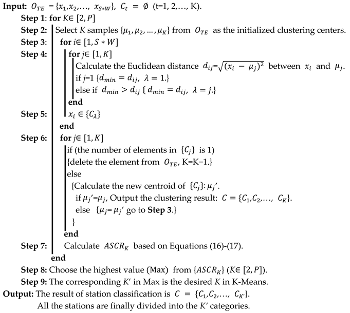
For example, if W = 5, five weekly passenger flow data have been used. If the ith station with the different five weekly passenger flows has been clustered into two categories, $N_i$ = 2 and $SC{R}_i$ = 1 − 2/5 = 0.6. If the ith station with the different five weekly passenger flows has been clustered into one category, $N_i$ = 1 and $SC{R}_i$ = 1 − 1/5 = 0.8. The optimized result is 0.8, which indicates that 5-week passenger flow at the same station has been clustered in the same category, and the clustering result is quite good. Then, average all $SC{R}_i$ as ASCR based on Equation (17). ASCR is the final evaluation result of all stations. It will be used to determine the number of categories for all stations, which is described in Section 3.4.1 in detail. The details of Algorithm 1 of K-Means for station classification are demonstrated below [11,12].

$C=\{C_1$,$C_2$,…,$C_K$} is the final result for station classification, and K′ is the number of categories. Notably, if the number of elements in $\left\{C_j\right\}$ is 1 in Step 6, this means that there is a separate category including only one station. This station will be deleted because it is unsuitable for the later prediction block for multi-station passenger flow prediction.

Algorithm 1: K-Means for station classification.

2.2. Prediction Block

A prediction block is used to predict the inflow for every type of station. $X_{S_i, T}\in {ℝ}^{S_i\times \left(M\times W\right)}$ is the input of the prediction block shown in Equation (18). By integrating the predicted passenger flow for every type of station, the final result $O_P$ for all the stations in the entire network will be obtained. The prediction block consists of three parts: spatial feature extraction, temporal feature extraction, and prediction.

$$X_{S_i, T}=\left\{\begin{array}{ccc}\begin{array}{cc}{x}_{1, t_1}& x_{1, t_2}\\ x_{2, t_1}& x_{2, t_2}\end{array}& \cdots & \begin{array}{c}{x}_{1, t_{M\times W}}\\ x_{2, t_{M\times W}}\end{array}\\ \begin{array}{cc}⋮ & ⋮\end{array}& \ddots & ⋮\\ \begin{array}{cc}{x}_{S_i, t_1}& x_{S_i, t_2}\end{array}& \cdots & x_{S_i, t_{M\times W}}\end{array}\right\}$$

(18)

where $S_i$ is the number of stations in the ith type of station, W is the number of weeks, and M = $DS\times days$ is the number of time intervals during a week. T = {t₁, t₂,…, $t_{M\times W}$} is a series of time intervals during a week.

2.2.1. Spatial Feature Extraction

(1)

Inflow

As shown in Figure 2, to better capture the spatial features, we extract three data modes from inflow data, namely real-time, daily, and weekly, from different periodicities in different time periods. The three types of data are shown in Equations (19)–(21).

$$X_{S_i,T}^R=\left\{\begin{array}{ccc}\begin{array}{cc}{x}_{1, t-n}^R& x_{1, t-n+1}^R\\ x_{2, t-n}^R& x_{2, t-n+1}^R\end{array}& \cdots & \begin{array}{c}{x}_{1, t-1}^R\\ x_{2, t-1}^R\end{array}\\ \begin{array}{cc}⋮ & ⋮\end{array}& \ddots & ⋮\\ \begin{array}{cc}{x}_{S_i, t-n}^R& x_{S_i, t-n+1}^R\end{array}& \cdots & x_{S_i, t-1}^R\end{array}\right\}$$

(19)

$$X_{S_i,T}^D=\left\{\begin{array}{ccc}\begin{array}{cc}{x}_{1, t-n-DS}^D& x_{1, t-n+1-DS}^D\\ x_{2, t-n-DS}^D& x_{2, t-n+1-DS}^D\end{array}& \cdots & \begin{array}{c}{x}_{1, t-1-DS}^D\\ x_{2, t-1-DS}^D\end{array}\\ \begin{array}{cc}⋮ & ⋮\end{array}& \ddots & ⋮\\ \begin{array}{cc}{x}_{S_i, t-n-DS}^D& x_{S_i, t-n+1-DS}^D\end{array}& \cdots & x_{S_i, t-1-DS}^D\end{array}\right\}$$

(20)

$$X_{S_i,T}^W=\left\{\begin{array}{ccc}\begin{array}{cc}{x}_{1, t-n-M}^W& x_{1, t-n+1-M}^W\\ x_{2, t-n-M}^W& x_{2, t-n+1-M}^W\end{array}& \cdots & \begin{array}{c}{x}_{1, t-1-M}^W\\ x_{2, t-1-M}^W\end{array}\\ \begin{array}{cc}⋮ & ⋮\end{array}& \ddots & ⋮\\ \begin{array}{cc}{x}_{S_i, t-n-M}^W& x_{S_i, t-n+1-M}^W\end{array}& \cdots & x_{S_i, t-1-M}^W\end{array}\right\}$$

(21)

$$I_{Inflow}=X_{S_i,T}^R\left|\left|X_{S_i,T}^D\right|\right|X_{S_i,T}^W$$

(22)

where $X_{S_i,T}^R$, $X_{S_i,T}^D$, $\mathrm{and}{X}_{S_i,T}^W$ represent the real-time, daily, and weekly inflow data, respectively. We use n historical time steps data {t − n, t − n + 1,…, t − 1} to predict the t time step inflow.

For example, t represents 9:00 am on Tuesday in the second week. $X_{S_i,T}^R$ refers to a series of inflow data of the first n time intervals before 9:00 am on Tuesday in the second week to predict the inflow at 9:00 am on Tuesday in the second week. $X_{S_i,T}^D$ refers to a series of inflow data of the first n time intervals before 9:00 am on Monday in the second week to predict the inflow at 9:00 am on Tuesday in the second week. $X_{S_i,T}^W$ refers to a series of inflow data of the first n time intervals before 9:00 am on Tuesday in the first week to predict the inflow at 9:00 am on Tuesday in the second week. Thus, T used in $X_{S_i,T}^R$, $X_{S_i,T}^D$, and $X_{S_i,T}^W$ is from the second week of training data. $X_{S_i,T}^R$, $X_{S_i,T}^D$, $\mathrm{and}{X}_{S_i,T}^W$ will be concatenated by column as the input $I_{Inflow}$ based on Equation (22).

As we know, deeper models can extract richer features [20], but it often brings risks of gradient disappearance and gradient explosion [7]. Therefore, some scholars proposed a residual network with jump links to solve this problem [21]. Residual connection reduces the complexity of the model to avoid overfitting, which is shown in Equation (23).

$${(O_{Inflow})}_{RB}=F\left({(I_{Inflow})}_{RB}\right)+{(I_{Inflow})}_{RB}$$

(23)

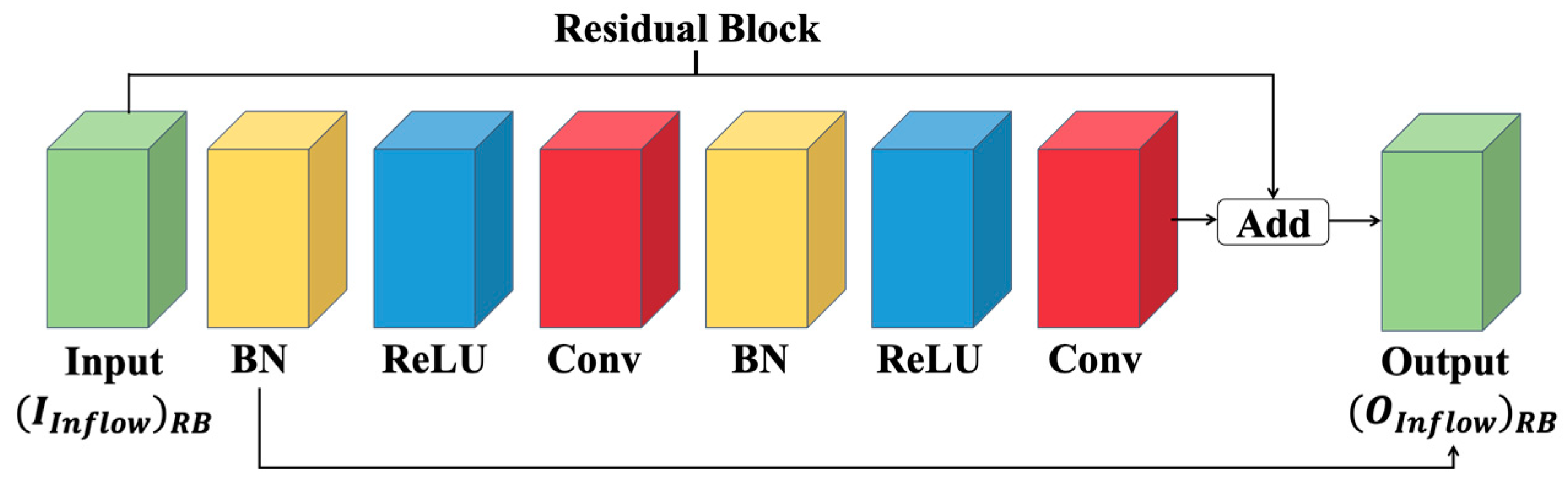
where ${(I_{Inflow})}_{RB}$ $\mathrm{and}{(O_{Inflow})}_{RB}$ refer to the input and output of the residual block, respectively. F(·) refers to the processing of the residual block, which is shown in Figure 3.

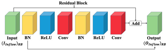
Figure 3. Processing of residual block.

As shown in Figure 3, the input ${(I_{Inflow})}_{RB}$ will go through a series of processing: BN represents batch normalization for data normalization, ReLU is an activation function, and Conv denotes a convolutional layer. Figure 2 shows two same-shape residual blocks used for inflow feature extraction. Then, the extracted features will be flattened and sent to a feed-forward network for full connection to extract the features based on Equations (13) and (14). $O_{P\_I}$ is the final output of inflow processing.

(2)

Outflow

The outflow processing is identical to the inflow processing. Hence, its final output is given by $O_{P\_O}$. $X_{S_i,T}^R$, $X_{S_i,T}^D$, $\mathrm{and}{X}_{S_i,T}^W$ represent the real-time, daily, and weekly outflow data, respectively.

(3)

Physical Topology

The physical topology is used to capture the topological information among the stations based on GCN for each type of station. Since the physical location of the stations is fixed, it is easy to construct an adjacent matrix A $\in {ℝ}^{{\mathrm{S}}_i\times {\mathrm{S}}_i}$, which is shown in Equations (24) and (25). We only consider the passenger flow in the real-time pattern ($X_{S_i,T}^R$) because the network topology does not change. The input of physical topology is defined as $I_{Topology}$ shown in Equation (26).

$$A=\left\{A^{\left|i,j\right|}\right\}$$

(24)

$$A^{\left|i,j\right|}=\left\{\begin{array}{c}1, station i and station j are adjacent\\ 0, otherwise\end{array}\right.$$

(25)

$$I_{Topology }=({\widehat{D}}^{-\frac{1}{2}}\widehat{A }{\widehat{D}}^{-\frac{1}{2}})\left(X_{S_i,T}^R\right)$$

(26)

where ${\widehat{D}}^{-\frac{1}{2}}\widehat{A }{\widehat{D}}^{-\frac{1}{2}}$ is the symmetric normalized Laplacian. $\widehat{A}=A+I$. $S_i$ refers to the number of stations in the ith type of station. I is the identity matrix, and $\widehat{D}$ is the diagonal node-degree matrix of $\widehat{A}$.

Then, we apply $I_{Topology}$ to a series of processing: two same-shape residual blocks, flattening, and full connection for further feature extraction. $O_{P\_Topo}$ is the final output of physical topology processing.

(4)

Spatial Feature Fusion

The extracted spatial features from inflow, outflow, and physical topology will be weighted fused as $O_{SF}$ based on Equation (27).

$$O_{SF}=W_1\circ O_{P\_I}+W_2\circ O_{P\_O}+W_3\circ O_{P\_Topo}$$

(27)

where $O_{P\_I}$, $O_{P\_O}$, $\mathrm{and}{O}_{P\_Topo}$ are the outputs of inflow, outflow, and physical topology, respectively. $W_1$, $W_2$, and $W_3$ are the trainable weights, respectively. The term “∘” denotes the Hadamard product.

2.2.2. Temporal Feature Extraction

$O_{SF}$ will be continuously sent to the attention LSTM and a fully connected network to obtain the temporal features. Attention LSTM is effective in predicting traffic flow [22,23,24]. Traditional conventional attention LSTM is used to capture the weight scores of different time intervals, usually by assigning heavier weight scores to adjacent time intervals and lower ones to those further apart [21]. However, passenger flow prediction models are affected by many factors, such as weather conditions [25], emergencies, passenger flow, network topology, and so on. Thus, applying the traditional conventional attention LSTM to assign weights for outputs in LSTM is insufficient. Therefore, based on previous work by Wu et al. [26], we use a fully connected network to obtain weights that can be scored according to the output of LSTM based on Equations (28) and (29).

$$\alpha =f\left(W\circ Out+b\right)$$

(28)

$$AttenLSTM=\alpha \circ Out$$

(29)

where $Out\in {ℝ}^{S_i\times Neu}$, $S_i$ refers to the number of stations in the ith category, and Neu represents the number of neurons used in LSTM. W is the trainable weights, b is the trainable bias, and f represents the activation function in the fully connected layer. The term $\alpha$ is a trainable weight matrix whose shape is identical to Out. The term “∘” denotes the Hadamard product. $AttenLSTM$ is the output of attention LSTM.

$AttenLSTM$ will be flattened and sent to a feed-forward network as $O_{FFN\_AttenLSTM}$ for full connection. $O_{FFN\_AttenLSTM}$ is the output of temporal feature abstraction, which is also the prediction result for the same type of station. Every type of station has the same processing to construct its own prediction model and obtain the corresponding prediction result. By integrating the predicted passenger flow for every type of station, the final result for all the stations in the whole network will be obtained.

3. Experiments

In this section, we introduce the two used datasets, the model configuration, the evaluation metrics, and the results of station classification and passenger flow prediction in the two datasets in the proposed (Transformer-K-Means)-(ResNet-GCN-AttLSTM) in detail.

3.1. Data Description

Two real-world ridership datasets are used to validate the effectiveness of the proposed (Transformer-K-Means)-(ResNet-GCN-AttLSTM): (1) the Beijing metro dataset, which is shared in [27]; (2) the Xiamen BRT dataset, which is collected from the BRT system in Xiamen, China. Because the Xiamen BRT adopts the closed viaduct mode, the mode of stations in the Xiamen BRT is similar with the stations in metro systems. Thus, we use the two datasets in our proposed model [28].

The details of these two datasets are summarized in Table 1. The dataset in the Beijing metro is from 29 February to 1 April 2016, which contains five continuous weekly inbound and outbound passenger flows. As of April 2016, there are a total of 17 lines covering 276 stations. The dataset in the Xiamen BRT is from 4 March to 5 April 2019, which contains five continuous weekly inbound and outbound passenger flows. Tomb Sweeping Day is on 5 April 2019, and is one of China’s traditional holidays. As of April 2019, a total of eight lines are covering 44 stations.

Table 1. Dataset Description.

Description	Beijing Metro			Xiamen BRT
Train Timespan	29/02/2016–04/03/2016 07/03/2016–11/03/2016 14/03/2016–18/03/2016 21/03/2016–25/03/2016			04/03/2019–08/03/2019 11/032019–15/03/2019 18/03/2019–22/03/2019 25/03/2019–29/03/2019
Test Timespan	28/03/2016–01/04/2016			01/04/2019–05/04/2019
Week Number	5			5
Day Number	25			25
Daily Service Hours	5:00 a.m.–11:00 p.m.			5:00 a.m.–11:00 p.m.
Time Interval	10 min	15 min	30 min	10 min	15 min	30 min
DS	108	72	36	108	72	36
Total DS	2700	1800	900	2700	1800	900
Line Number	17			8
Station Number	276			44

Consequently, station-level passenger flow in the Beijing metro is much more complex than it in the Xiamen BRT. To avoid the influence of passenger flow at weekends, we only choose the passenger flow on workdays for study. The total five weekly inflow and outflow data are used in the classification block. The first four weekly data are for training, and the last week’s data are for testing in the prediction block. The time intervals used in the two datasets are 10 min, 15 min, and 30 min, respectively. The two datasets’ daily service hours are from 5:00 a.m. to 11:00 p.m., with both containing 18 h. Thus, DS in different time intervals is different, which is shown in Table 1.

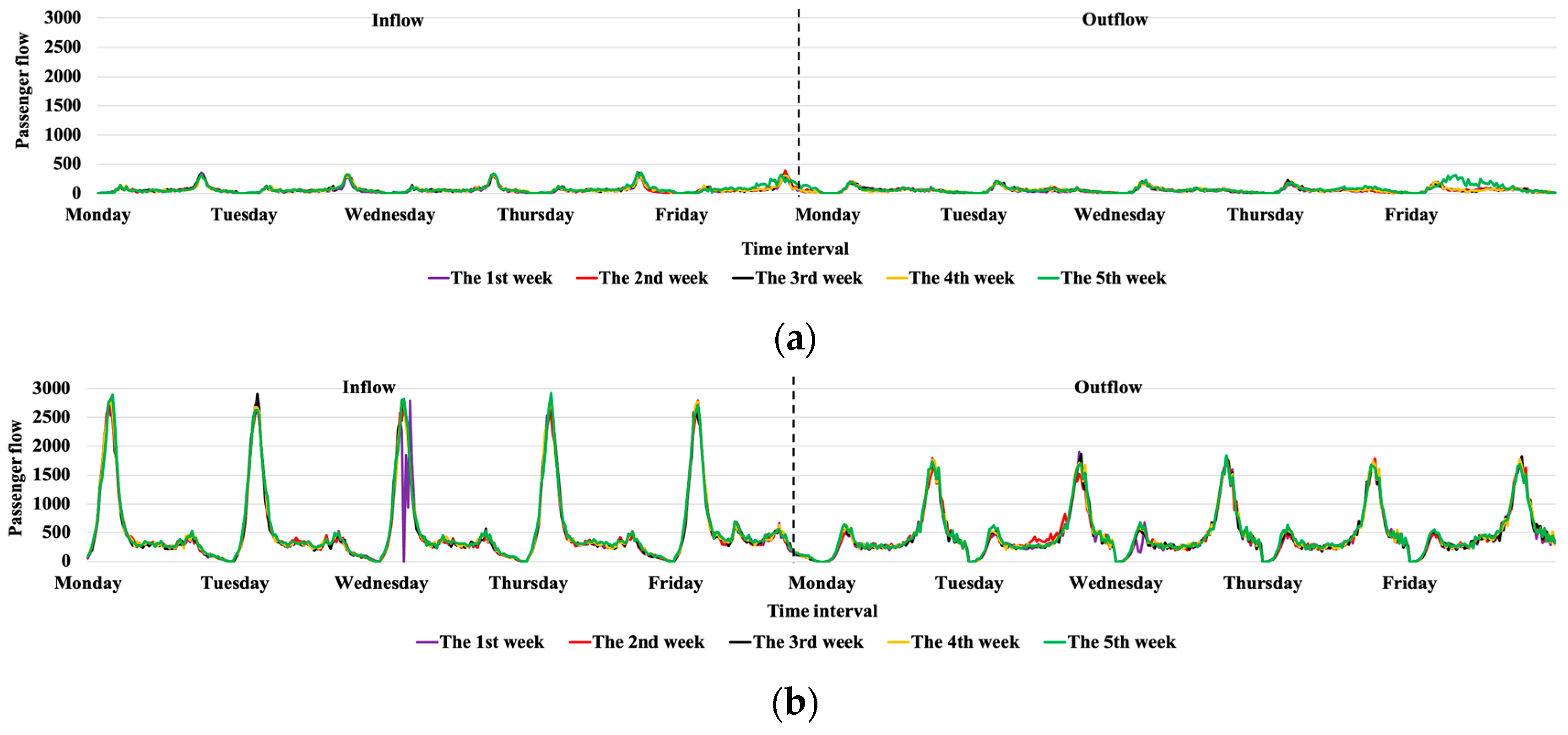
As shown in Figure 4, the real-time, daily, and weekly inflow and outflow at 1st Wharf Station in the Xiamen BRT and No. 1 Station in the Beijing metro during the five workdays are quite different. Different weekly ridership at the same station is periodic and stable. It verifies that using the three types of data modes (real-time, daily, weekly) for temporal feature extraction is useful in our proposed model.

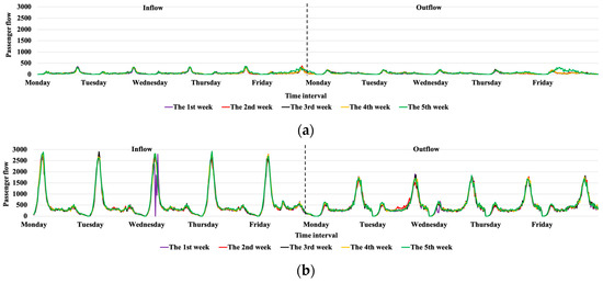
Figure 4. Stations’ passenger flow in the Xiamen BRT and the Beijing metro. (a) Five weekly inflow and outflow at 1st Wharf Station in the Xiamen BRT. (b) Five weekly inflow and outflow at No.1 Station in the Beijing metro.

Moreover, as shown in Figure 1 and Figure 4, the inflow and outflow at the same station are also different. For example, No. 1 Station in the Beijing metro has a larger inflow, while there is a smaller outflow in Figure 4b. Xianhou Station in the Xiamen BRT has a smaller inbound flow, and a larger outbound flow in Figure 1a. The inflow and outflow at Dongzhai Station in Figure 1b are quite similar to the flows at 1st Wharf Station in Figure 4a in the Xiamen BRT. Consequently, before passenger flow prediction, it is significant to classify the stations based on passenger flow similarity.

3.2. Model Configuration

Compared with outflow, inflow is more likely to cause congestion in UPT. Additionally, the inflow is more regular than the outflow [4]. Thus, we choose the historical five ahead-of-time interval inflow and outflow data as the inputs to predict the next one-time-step inflow in our experiment. The parameters used in the classification and prediction blocks are specified in Table 2 and Table 3, respectively. $S_i$ is the number of stations used in the prediction model in Table 3.

Table 2. Parameters used in the classification block.

Parameters	Transformer Encoder	K-Means
d_model	2 × DS, 2 × days
Number of heads	2
K		2–10
Optimizer	Adam
Learning rate	0.00004

Table 3. Parameters used in the prediction block.

Parameters	Inflow	Outflow	Physical Topology	Attention LSTM
Kernel Size	3 × 3	3 × 3	3 × 3
Residual Block 1	32 filters	32 filters	32 filters
Residual Block 2	64 filters	64 filters	64 filters
Batch Size	64	64	64	64
Activation Function	Relu	Relu	Relu	Linear
Number of Neurons in FC 1	$S_i$	$S_i$	$S_i$
Number of Neurons in FC 2				$S_i$
Number of Layers				1
Number of Neurons (Neu)				128

3.3. Evaluation Metrics

To evaluate the classification performance of the proposed model, we use A$SCR$ as an evaluation metric, which is shown in Equation (17). The passenger flow at the same category of stations is also visualized to evaluate the performance, too.

The three common evaluation metrics, including mean square error (RMSE), mean absolute error (MAE), and weighted mean absolute percentage error (WMAPE), are used for evaluating the prediction performance. They are defined in Equations (30) and (32). The smaller the metrics are, the better the results.

Mean squared error (MSE) is used as the loss function in Equation (33).

$$RMSE=\sqrt{\frac{1}{S}{{\displaystyle \sum }}_{i=1}^S{\left(y_i-{\widehat{y}}_i\right)}^2}$$

(30)

$$MAE=\frac{1}{S}{{\displaystyle \sum }}_{i=1}^S\left|y_i-{\widehat{y}}_i\right|$$

(31)

$$WMAPE\left(\%\right)={{\displaystyle \sum }}_{i=1}^S\left(\frac{y_i}{{{\displaystyle \sum }}_{i=1}^S{y}_i}\left|\frac{y_i-{\widehat{y}}_i}{y_i}\right|\right)$$

(32)

$$MSE=\frac{1}{S}{{\displaystyle \sum }}_{i=1}^S{(y_i-{\widehat{y}}_i)}^2$$

(33)

where $y_i$ is the real passenger flow, and ${\widehat{y}}_i$ is the predicted passenger flow. For unclassified prediction, S is the total number of stations in the whole network. For classified prediction, S is the number of stations in the same category.

To integrate the passenger flow prediction results for every type of station, RMSE, MAE, and WMAPE are redefined as Equations (34) and (36).

$$RMSE=\sqrt{\frac{1}{S}{{\displaystyle \sum }}_{i=1}^{K^{\prime }}RMS{E}_i^2\times S_i}$$

(34)

$$MAE=\frac{1}{S}{{\displaystyle \sum }}_{i=1}^{K^{\prime }}MA{E}_i\times S_i$$

(35)

$$WMAPE=\frac{1}{{{\displaystyle \sum }}_{i=1}^S{y}_i}{{\displaystyle \sum }}_{i=1}^{K^{\prime }}(WMAP{E}_i\times ({{\displaystyle \sum }}_{i=1}^{S_i}{y}_i))$$

(36)

where $K^{\prime }$ is the number of categories for stations in the whole network, $S_i$ is the number of the ith type of station, S is the total number of stations in the whole network, and $y_i$ is the passenger number of the ith station.

3.4. Experiment Results

In this section, the results of station classification and passenger flow prediction in the two datasets have been present and discussed in detail.

3.4.1. Classification Results

ASCR with different K in different time intervals in the Xiamen BRT and the Beijing Metro are shown in Table 4. The numbers in bold refer the best results in different values of K. Since the Xiamen BRT network is much simpler than the Beijing metro network, the situations with the highest ASCR = 0.8 are more than those in the Beijing metro.

Table 4. ASCR with different K in the Xiamen BRT and the Beijing Metro.

K	ASCR
	Xiamen BRT			Beijing Metro
	10 min	15 min	30 min	10 min	15 min	30 min
2	0.8	0.8	0.795	0.794	0.797	0.797
3	0.8	0.795	0.795	0.8	0.797	0.797
4	0.8	0.8	0.8	0.787	0.798	0.798
5	0.8	0.795	0.795	0.791	0.796	0.795
6	0.8	0.795	0.795	0.782	0.792	0.793
7	0.789	0.790	0.8	0.786	0.791	0.790
8	0.794	0.785	0.8	0.785	0.789	0.792
9	0.8	0.795	0.795	0.781	0.788	0.790
10	0.784	0.790	0.795	0.781	0.788	0.790

For 10 min, 15 min, and 30 min time intervals in the Xiamen BRT, we choose K = 4 as the final number of categories for station classification. Because of the fact that when K is 4, the ASCR of all categories is 0.8, which is a more stable result. For 10 min, 15 min, and 30 min time intervals in the Beijing Metro, we choose K = 3, 4, 4 as the classification results, respectively. The classification results show that with more data, the number of station categories will not be too large.

It is notable that only the station number is provided for the Beijing metro; we cannot list the stations’ names. More information about the Beijing metro can be found in [27]. The names of the stations in the Xiamen BRT are listed in Table 5 [29]. We only list the station classification results for the Xiamen BRT in 15 min time interval as an example. The station classification results are shown in Table 6, and the visualization of inflow from 3 April 2019 to 8 April 2019 in the four categories of stations is shown in Figure 5.

Table 5. Names of stations in the Xiamen BRT.

No.	Station Name	No.	Station Name	No.	Station Name	No.	Station Name
1	1st Wharf	12	Caitang	23	Dongzhai	34	Pantu
2	Kaihe Intersection	13	Jinshan	24	Tiancuo	35	Binhai Xincheng (Xike) Junction
3	Sibei	14	Municipal Administrative Service Center	25	Xiamen North Railway Station	36	Guanxun
4	Douxi Road	15	Shuangshi Middle School	26	Institute of Technovation	37	Light Industry and Food Park
5	Ershi	16	Xianhou	27	Gaoqi Airport	38	Sikouzhen
6	Jinbang Park	17	Airport Terminal 4	28	Fenglin	39	Industrial Zone
7	Railway Station	18	Tan Kah Kee Stadium	29	Dong’an	40	3rd Hospital
8	Lianban	19	Chengyi University College	30	Houtian	41	Chengnan
9	Longshanqiao	20	Huaqiao University	31	Dongting	42	Tong’an Junction
10	Wolong Xiaocheng	21	University Town	32	Meifeng	43	Hongwen
11	Dongfang Shanzhuang	22	Chinese Academy of Sciences	33	Caidian	44	Qianpu Junction

Table 6. Station classification results in the Xiamen BRT in 15 min time interval.

Categories	Station No.	Number	Passenger Flow Volume
1	21, 22, 23, 24, 26, 27, 28, 29, 30, 31, 32, 33, 34, 35, 37, 38, 40	17	Small
2	1, 9, 11, 17, 19, 20, 36, 39, 41, 42	10	Medium
3	2, 3, 4, 5, 6, 8, 43	7	Medium
4	10, 12, 13, 15, 16, 18	6	Large

Figure 5. Visualization of inflow in the four categories of stations in 15 min time interval in the Xiamen BRT. (a) Inflow visualization in the first category; (b) inflow visualization in the second category; (c) inflow visualization in the third category; (d) inflow visualization in the fourth category.

As shown in Figure 5, Railway Station (No. 7), Municipal Administrative Service Center Station (No. 14), Xiamen North Railway Station (No. 25), and Qianpu Junction Station (No. 44) have been divided into separate categories. Thus, the four stations have been deleted in our model based on the following Algorithm 1: K-Means for station classification. All four stations are importation stations because of their urban functions and geographical position. Therefore, there are 40 stations in the Xiamen BRT that have been used for classification and prediction, which are divided into four categories in 15 min time intervals. The max volume of inflow at the first category of stations is less than 300, which are defined as the small ridership stations. The max volume of inflow at the second and third category of stations is less than 520, and these stations are defined as the medium ridership stations. The max volume of inflow at the fourth category of stations is less than 800, which are defined as large ridership stations. The weekly inflow in the four categories of stations has regular periodicity, such as similar morning and evening peaks and the same change curves.

Table 7 shows the deleted stations in the different time intervals in the Xiamen BRT. The larger the time interval is, the less the deleted stations are. It verifies that the passenger flow will be become more regular when the time interval increases. Station classification may be a more necessary strategy for short-term passenger flow prediction.

Table 7. The deleted stations in the different time intervals in the Xiamen BRT.

No.	Deleted Station	Time Interval
		10 min	15 min	30 min
3	Sibei	✓
7	Railway Station	✓	✓	✓
14	Municipal Administrative Service Center	✓	✓
25	Xiamen North Railway Station	✓	✓	✓
44	Qianpu Junction	✓	✓	✓

“✓” refers the deleted stations in different time intervals.

Moreover, the stations in the Beijing metro with 276 stations have not been deleted. It verifies that station classification may be more significant for a larger dataset.

The No. 34 station is Pantu Station, shown in Figure 5a. Since there are two schools near the station, the inbound passenger flow increases sharply at noon and in the afternoon during the peak periods of school and after school. However, during class hours, the passenger flow at this station is the same as usual. The station classification in the proposed model is based on the inflow and outflow at all time intervals during a week. Therefore, the different changes of flows in several time intervals will not affect the classification results. It verifies the effectiveness of the classification block in the proposed model based on the Transformer encoder and K-Means.

3.4.2. Prediction Results in the Beijing Metro

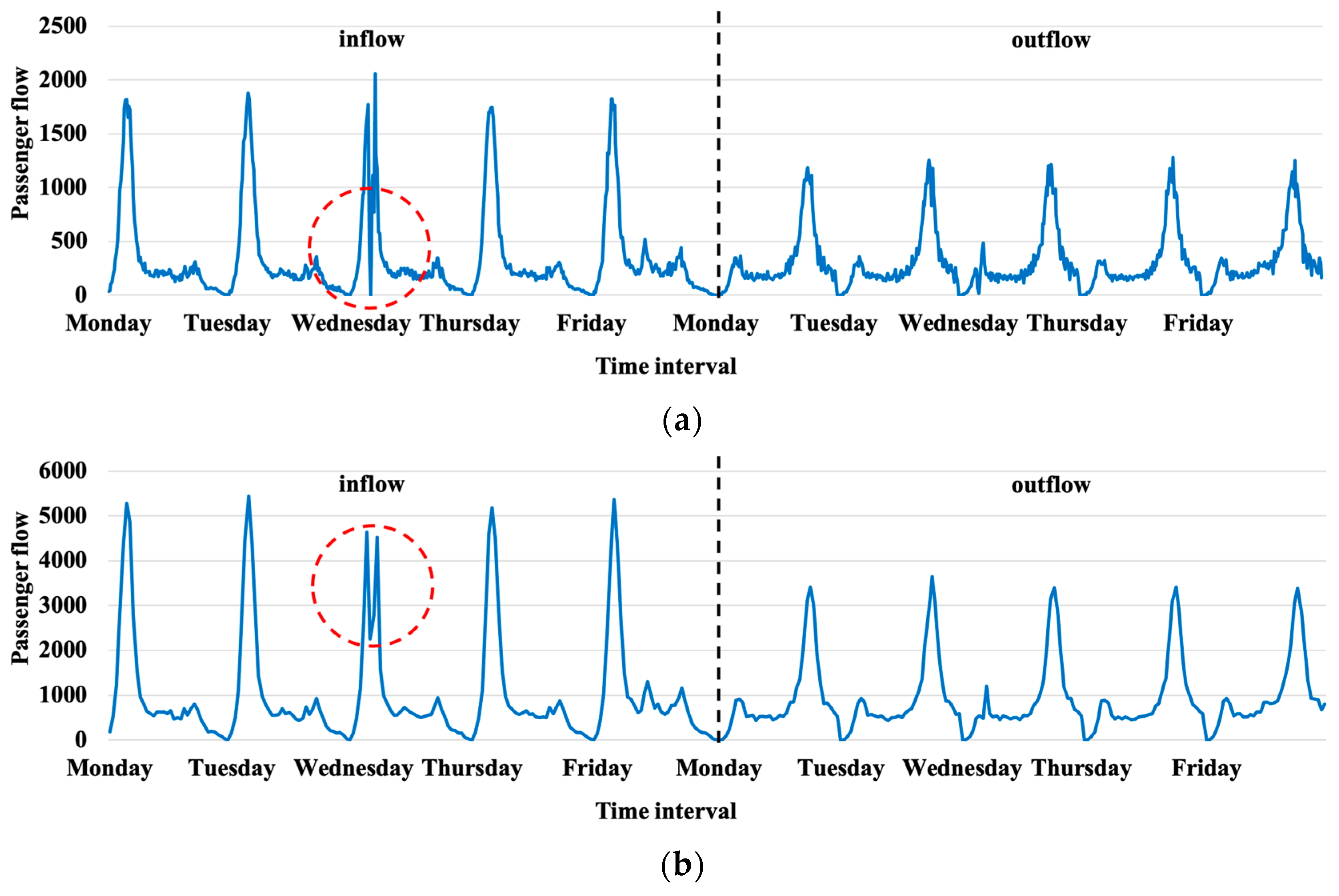
The performance of prediction results in different time intervals in the Beijing metro is summarized in Table 8. The numbers in bold refer the better results between prediction with station classification, and prediction without station classification. The prediction results of MAE, RMSE, and WMAPE with classification in 15 min and 30 min time intervals are better than the prediction results without classification. Only RMSE in 10 min time intervals presents a slightly worse performance. It may be affected by an emergency, which causes the volume of inflow to suddenly decrease at some stations. This influence is more obvious for the passenger flow in smaller time intervals. Take the inflow at No.1 Stations in the Beijing metro, for example. Figure 6a,b illustrates the inflow and outflow in 10 min and 30 min time intervals, respectively. The inflow with a 10 min time interval clearly shows that the flow suddenly drops to zero shown in the dashed circle in Figure 6a. When the time interval increases to 30 min, the passenger flow is substantially reduced caused by the passenger flow dropped sharply to zero in the 10 min time interval, which is shown in the dashed circle in Figure 6b. Because RMSE is more affected by such outliers, poor RMSE results occur, especially in the scenario of 10 min time interval.

Table 8. Prediction results in the Beijing Metro.

Time Interval	Prediction Mode	Metrics
		MAE	RMSE	WMAPE
10 min	Prediction (with classification)	17.2781	29.6929	9.668%
	Prediction (w/o classification)	17.6344	29.6219	9.911%
15 min	Prediction (with classification)	22.1919	37.9693	8.269%
	Prediction (w/o classification)	23.0008	38.7386	8.589%
30 min	Prediction (with classification)	32.5245	58.1694	6.120%
	Prediction (w/o classification)	34.1360	60.1340	6.428%

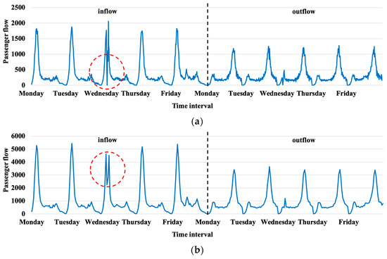
Figure 6. Inflow at No.1 Stations in the Beijing metro. (a) 10 min time interval; (b) 30 min time interval.

In summary, classification can still improve the prediction results for a suddenly decreasing flow. In most scenarios, the larger the time interval is, the better the improvement effects.

3.4.3. Prediction Results in the Xiamen BRT

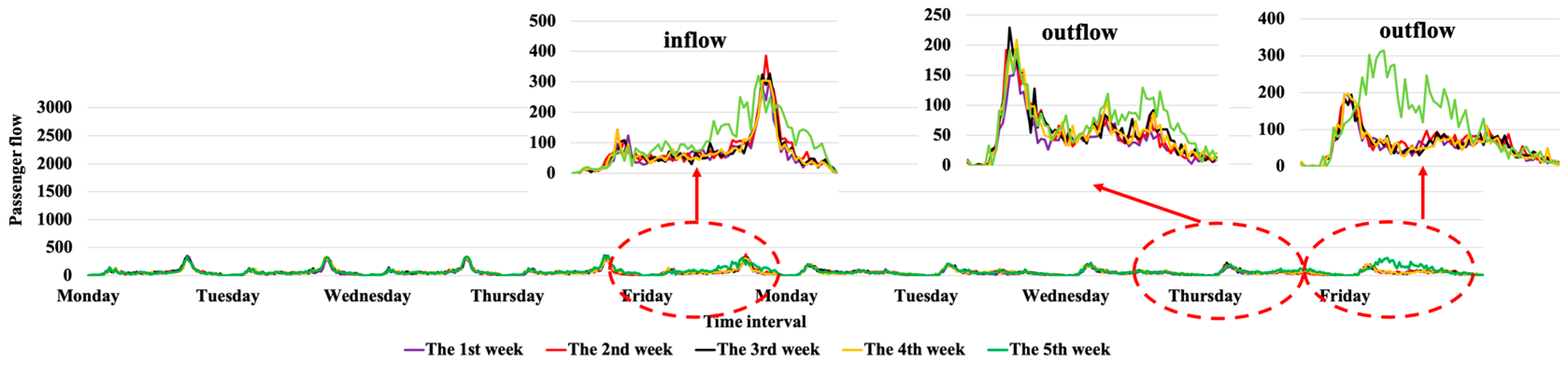
The testing dataset includes Tomb Sweeping Day on 5 April 2019 in the Xiamen BRT, which is Friday in the fifth week. As shown in Figure 7, the inflow and outflow on the holiday included in the three-dotted red boxes are quite different from that on normal days. The inflow in the morning and evening peaks is slightly less than that on normal days, and the inflow in other hours is slightly more than that in normal times. The outflow on that day and even the day before is much more than usual. It is mainly because there is a ferry terminal near 1st Wharf Station, and a famous place of interest, Gulangyu island, is on the opposite side. Therefore, people who travel to it will choose a more convenient public transport, i.e., the BRT, which causes a sharp increase in outbound flow.

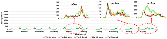
Figure 7. Inflow and outflow at 1st Wharf Station in the Xiamen BRT on Tomb Sweeping Day.

The performance of prediction results in different time intervals in the Xiamen BRT is summarized in Table 9. The numbers in bold refer the better results between prediction with station classification, and prediction without station classification. The prediction results of MAE, RMSE, and WMAPE with classification in 10 min and 15 min time intervals are better than the prediction results without classification. Only MAE and WMAPE in 30 min time interval presents a slightly poorer performance. This is mainly because there is less abnormal flow included on this holiday in 10 min and 15 min time intervals, so a classified prediction can show a better performance. Under the 30 min time granularity, more irregular flow data are included, and the irregular flow cannot be well extracted through classification, which leads to an unsatisfactory prediction performance. In the end, in the most scenarios, classification can still improve the prediction result for suddenly increasing flows on holiday. The smaller the time interval is, the better the improvement effects are in the most scenarios.

Table 9. Prediction results in the Xiamen BRT.

Time Interval	Prediction Mode	Metrics
		MAE	RMSE	WMAPE
10 min	Prediction (with classification)	9.2998	15.6633	18.58%
	Prediction (w/o classification)	9.3990	16.0151	18.80%
15 min	Prediction (with classification)	12.7193	22.2835	16.29%
	Prediction (w/o classification)	12.7559	22.3270	16.33%
30 min	Prediction (with classification)	23.0463	46.2256	14.26%
	Prediction (w/o classification)	22.6983	47.2300	14.03%

4. Conclusions

As far as we know, most existing studies mainly focused on spatio-temporal feature extraction to construct a multi-station passenger flow prediction model by using different deep learning models. Different from the previous studies, we have proposed a novel two-step strategy, namely classification followed by prediction, to develop a better performance model for multi-station passenger flow prediction. Two different complex real-world ridership datasets have been used to demonstrate the effectiveness of the proposed model. Compared with the unclassified results, the proposed model (Transformer-K-Means)-(ResNet-GCN-AttLSTM) with station classification presents a better performance in multi-station passenger flow prediction. As far as we know, this is the first time station classification has been added into multi-station passenger flow prediction, which presents good performance.

Improvements can be made in future work. One issue is in developing a more advanced multi-station passenger flow prediction model by better extracting the complex spatio-temporal features, such as using the fractal-wavelet modeling [30,31,32,33,34,35]. Another one is in combining the classification block with more state-of-the-art models to verify the effectiveness of station classification in multi-station passenger flow prediction.

References

- Zhang, Z.; Han, Y.; Peng, T.; Li, Z.; Chen, G. A comprehensive spatio-temporal model for subway passenger flow prediction. ISPRS Int. J. Geo-Inf. 2022, 11, 341. [Google Scholar] [CrossRef]
- Li, X.C.; Peng, Y.Z.; Wu, Z.X.; Chen, Z.W. Short-term forecast of metro station passenger flow based on deep spatial-temporal network. Traffic Transp. 2020, 33, 55–61. [Google Scholar]
- Zhang, J.L. Study of the Short-Term Passenger Flow Prediction in Urban Rail Transit Networks. Ph.D. Thesis, Beijing Jiaotong University, Beijing, China, 29 May 2021. [Google Scholar]
- Zhao, Y.J.; Lin, Y.F.; Zhang, Y.K.; Wen, H.M.; Liu, Y.X.; Wu, H.; Wu, Z.H.; Zhang, S.C.; Wan, H.Y. Traffic inflow and outflow forecasting by modeling intra- and inter-relationship between flows. IEEE Transp. Intell. Transp. Syst. 2022, 23, 20202–20216. [Google Scholar] [CrossRef]
- Bogaerts, T.; Masegosa, A.D.; Angarita-Zapata, J.S.; Onieva, E.; Hellinckx, P. A graph CNN-LSTM neural network for short and long-term traffic forecasting based on trajectory data. Transp. Res. Part C Emerg. Technol. 2020, 112, 62–77. [Google Scholar] [CrossRef]
- Li, S.; Wang, Q.W.; Chen, Y.R.; Qin, J. Prediction of short-time passenger flow on multi-station urban rail based on SAE-ConvLSTM deep learning model. Appl. Res. Comput. 2022, 39, 2025–2031. [Google Scholar]
- Zhang, S.X.; Zhang, J.L.; Yang, L.X.; Yin, J.T.; Gao, Z.Y. GCN-Transformer for short-term passenger flow prediction on holidays in urban rail transit systems. arXiv 2022, arXiv:2203.00007v3. [Google Scholar]
- Ma, C.Q.; Li, P.K.; Zhu, C.H.; Lu, W.B.; Tian, T. Short-term passenger flow forecast of urban rail transit based on different time granularities. J. Chang’an Univ. Nat. Sci. Ed. 2020, 40, 75–83. [Google Scholar]
- Du, C.L.; Li, X.L.; Sun, R.R.; Zhang, P.; Zhu, G.Y. Classification of urban rail station based on passenger flow congestion propagation. J. Beijing Jiaotong Univ. 2021, 45, 39–46. [Google Scholar]
- Wang, H.D.; Ma, H.W. Classification method of urban rail transit stations based on POI. Traffic Transp. 2020, 36, 33–37. [Google Scholar]
- Xia, X.; Gai, J.Y. Classification of urban rail transit stations and points and analysis of passenger flow characteristics based on K-Means clustering algorithm. Modern Urban Transit. 2021, 4, 112–118. [Google Scholar]
- Zhao, Y.; Wang, Y.; Hu, H. Research on clustering method of metro stations based on POI-K_Means. Intell. Comput. Appl. 2022, 12, 114–118. [Google Scholar]
- Yuan, F.T.; Chen, T.J.; Wei, J.B. Research on classification of rail stations based on AFC data. J. Transp. Eng. 2021, 21, 48–52, 57. [Google Scholar]
- Jiang, Y.S.; Yu, G.S.; Hu, L.; Li, Y. Refined classification of urban rail transit stations based on clustered station’s passenger traffic flow features. J. Transp. Syst. Eng. Inf. Technol. 2022, 22, 106–112. [Google Scholar]
- Wang, W.Y.; Liu, J.C.; Yu, Y.D. Research on classification of Xi’an rail transit stations based on land use and population. People’s Public Transp. 2020, 8, 29–33. [Google Scholar]
- Vaswani, A.; Shazeer, N.; Parmar, N.; Uszkoreit, J.; Jones, L.; Gomez, A.N.; Kaiser, L. Attention is all you need. In Proceedings of the 31st Conference on Neural Information Processing Systems (NIPS 2017), Long Beach, CA, USA, 4 December 2017. [Google Scholar]
- Wang, Q.W.; Chen, Y.R.; Liu, Y.C. Metro short-term traffic flow prediction with ConvLSTM. Contral Decis. 2021, 36, 2760–2770. [Google Scholar]
- Tan, Y.F.; Liu, H.X.; Pu, Y.; Wu, X.M.; Jiao, Y.B. Passenger flow prediction of integrated passenger terminal based on K-Means-GRNN. J. Adv. Transp. 2021, 10, 1055910. [Google Scholar] [CrossRef]
- Hinton, G.E.; Osindero, S.; The, Y.W. A fast learning algorithm for deep belief nets. Neural Comput. 2006, 18, 1527–1554. [Google Scholar] [CrossRef]
- Szegedy, C.; Liu, W.; Jia, Y.Q.; Sermanet, P.; Reed, S.; Anguelov, D.; Erhan, D.; Vanhoucke, V.; Rabinovich, A. Going deeper with convolutions. In Proceedings of the IEEE Conference on Computer Vision and Pattern Recognition (CVPR 2015), Boston, MA, USA, 8–10 June 2015. [Google Scholar]
- He., K.M.; Zhang, X.Y.; Ren, S.Q.; Sun, J. Deep residual learning for image recognition. In Proceedings of the IEEE Conference on Computer Vision and Pattern Recognition (CVPR 2016), Las Vegas, NV, USA, 26 June–1 July 2016. [Google Scholar]
- Wang, J.X.; Wang, R.; Zeng, X. Short-term passenger flow forecasting using CEEMDAN meshed CNN-LSTM-attention model under wireless sensor network. IET Commun. 2022, 16, 1253–1263. [Google Scholar] [CrossRef]
- Yang, J.; Dong, X.; Jin, S. Metro passenger flow prediction model using attention-based neural network. IEEE Access 2020, 8, 30953–30959. [Google Scholar] [CrossRef]
- Xue, G.; Liu, S.F.; Ren, L.; Ma, Y.C.; Gong, D.Q. Forecasting the subway passenger flow under event occurrences with multivariate disturbances. Expert Syst. Appl. 2022, 188, 116057–116070. [Google Scholar] [CrossRef]
- Liu, L.J.; Chen, R.C.; Zhu, S.Z. Impacts of weather on short-term metro passenger flow forecasting using a deep LSTM neural network. Appl. Sci. 2020, 10, 2926. [Google Scholar] [CrossRef]
- Wu, Y.K.; Tan, H.C.; Qin, L.Q.; Ran, B.; Jiang, Z.X. A hybrid deep learning based traffic flow prediction method and its understanding. Transp. Res. Part C Emerg. Technol. 2018, 90, 166–180. [Google Scholar] [CrossRef]
- Zhang, J.; Chen, F.; Cui, Z.; Guo, Y.; Zhu, Y. Deep learning architecture for short-term passenger flow forecasting in urban rail transit. IEEE Transp. Intell. Transp. Syst. 2021, 22, 7004–7014. [Google Scholar] [CrossRef]
- Chen, L.; Liu, L.J.; Yuan, L. Multi-head attention mechanism for multi-station passenger flow prediction. In Proceedings of the 2022 International Symposium on Design Studies and Intelligence Engineering (DSIE2022), Hangzhou, China, 29–30 October 2022. [Google Scholar]
- The Most Authoritative Route Map of Xiamen BRT. Available online: http://xm.bendibao.com/traffic/20161011/51844.shtm (accessed on 29 July 2022).
- Siwar, Y.; Salwa, S.; Mourad, Z. Wavelet extreme learning machine and deep learning for data classification. Neurocomputing 2022, 470, 280–289. [Google Scholar]
- Emanuel, G.; Rodrigo, C. Chebyshev wavelet analysis. J. Funct. Spaces 2022, 2022, 5542054. [Google Scholar]
- Gökalp, Ç.; Bülent, G.E.; Ahmet, H.Y. Prediction of glioma grades using deep learning with wavelet radiomic features. Appl. Sci. 2020, 10, 6296. [Google Scholar]
- Yu, X.J.; Liu, Y.R.; Sun, Z.M.; Qin, P. Wavelet-based ResNet: A deep-learning model for prediction of significant wave height. IEEE Access 2022, 10, 110026–110033. [Google Scholar] [CrossRef]
- Emanuel, G.; Sergei, S. Fractional-wavelet analysis of positive definite distributions and wavelets on D′(C). In Engineering Mathematics II: Algebraic, Stochastic and Analysis Structures for Networks, Data Classification and Optimization; Sringer Proceedings in Mathematics & Statistics; Springer International Publishing: New York, NY, USA, 2016; Volume 179, pp. 337–353. [Google Scholar]
- Indumathi, J.; Kaliraj, V. Petite term traffic flow prediction using deep learning for augmented flow of vehicles. Concurr. Eng. 2022, 30, 214–224. [Google Scholar] [CrossRef]
Disclaimer/Publisher’s Note: The statements, opinions and data contained in all publications are solely those of the individual author(s) and contributor(s) and not of MDPI and/or the editor(s). MDPI and/or the editor(s) disclaim responsibility for any injury to people or property resulting from any ideas, methods, instructions or products referred to in the content. |
© 2023 by the authors. Licensee MDPI, Basel, Switzerland. This article is an open access article distributed under the terms and conditions of the Creative Commons Attribution (CC BY) license (https://creativecommons.org/licenses/by/4.0/).