Mathematical Models for Predicting the Elastic and Thermal Behavior of Heterogeneous Materials through Curve Fitting

Abstract

The aim of this study is to establish a new method for predicting the effective elastic and thermal behavior of heterogeneous materials through mathematical curve fitting. The research initiates with the collection of 3D microstructures comprising 200 spherical inclusions embedded within a linear elastic matrix. This database is acquired by varying the volume fraction of the inclusions (10%, 15%, 20%, or 25%) and the contrast between the two phases. The contrast is quantified in terms of the ratio of the Young’s modulus and thermal conductivity modulus, $\frac{E_i}{E_m}$ and $\frac{{\lambda }_i}{{\lambda }_m}$, with values ranging from 10 to 200. These microstructures are then used to estimate the elastic and thermal properties by calculating the effective bulk, shear, and thermal conductivity moduli via the finite element method (FEM). The compiled database is a crucial asset for the development of mathematical equations that precisely fit the curves of various moduli based on changes to input parameters such as the volume fraction and the contrast. The process includes analyzing the data, identifying patterns, and establishing mathematical relationships that effectively reflect the moduli’s observed behavior. By integrating these individual equations and taking into account their interdependencies, the resultant comprehensive 3D model provides an extensive representation of the material’s behavior and takes into consideration the impacts of varying the volume fraction and contrast on the different moduli. This approach enables a better understanding of the material’s response under diverse conditions. Results exhibit the accuracy and reliability of the chosen mapping functions and parameters. Thereby, these proposed functions, with respect to boundary conditions and analytical limits, confirm the relevance of the proposed model to capture such information with a suitable level of precision.

1. Introduction

Heterogeneous and composite materials [1,2,3] are increasingly used in various industrial sectors, notably in the aerospace and automotive industries. Despite their growing popularity, the full potential of these materials is yet to be fully realized, mostly due to their inherent variability and complex microstructural morphologies.

Accurate prediction of composite performance and heterogeneous materials, which exhibit a wide range of arrangements and morphologies of heterogeneities, is a challenging task. Solely relying on experimental and analytical homogenization approaches [4,5,6], based on either real [7] or virtual [8,9] microstructures, proves to be excessively time-consuming and resource-intensive. However, a viable approach is to utilize experimental data to create a multitude of random yet statistically equivalent virtual microstructures. The primary goal of this approach is to methodically predict the macroscopic behavior of these materials, taking into account the complexities and variations inherent in their structures.

Given the broad spectrum of materials requiring analysis, the use of curve fitting [10] and mathematical modeling [11] is indispensable for constructing homogenized behavioral models. These models, when efficiently optimized, can accurately determine critical parameters such as shape, volume fraction, and contrast. Applying curve-fitting techniques enables us to efficiently exploit a massive database of materials to develop refined and optimized macroscopic behavioral models.

Over the last few years, several experimental studies have leveraged curve fitting to predict mechanical and thermal properties of heterogeneous materials. Bourih and Kaddouri [12] employed this methodology to estimate the effective thermal conductivity of Lotus-type porous materials (LTPM) by delineating the characteristics of each phase according to its unique porous morphology. The model’s efficiency was thoroughly investigated in light of results obtained using finite element homogenization methods. This methodological precision not only facilitated the accurate prediction of LTPM thermal conductivity but also proved its reliability and applicability through a rigorous validation process in relation to standard computational methods.

As an extension of this method, Kaddouri and El Moumen [13] have taken advantage of the capabilities of curve fitting to develop a sophisticated mathematical model specifically designed for estimating thermal conductivity in two-phase heterogeneous two-dimensional materials. Their study stood out for its comprehensive approach, in which model predictions were rigorously evaluated against established analytical benchmarks, including series, parallel, and Maxwell models. This meticulous comparative analysis not only highlighted the efficiency and accuracy of their curve-fitted model but also showed its potential in capturing the complex thermal behavior of these materials.

Rajinder [14] made a significant contribution by developing four distinct mathematical models for estimating the relative Young’s moduli of materials. The first two models incorporated three essential variables: the contrast between the two phases and the Poisson’s coefficient. Relying on this foundation, the latter two models introduced an additional parameter—the volume fraction of particle packing—with the aim of enhancing the precision of predictions. What sets these models apart is not only their mathematical sophistication but also their practical utility, as Rajinder meticulously validated the models’ efficiency through a comprehensive comparison with experimental data.

In their pioneering work, Moran and Ning [15] introduced a sophisticated mathematical method designed to ascertain the elastic properties of composite materials featuring multiple phases. Their innovative approach relied on advanced numerical techniques to analyze stress–strain relationships, with a particular emphasis on unraveling the intricate influence of pores (voids) on the material’s behavior. Despite their limited quantity, these seemingly minute voids exerted a substantial impact on the overall properties of the composite material, a phenomenon that Moran and Ning systematically explored and elucidated.

In a noteworthy study, Rackel [16] undertook the application of curve-fitting techniques to assess the performance of three distinct hyperelastic models: the Yeoh model [17], the Orgen model [18], and a polynomial model. The central aim of this investigation was to predict both the compressibility and shear moduli by establishing comprehensive stress–strain relationships. Relying on curve fitting, Rackel sought to analyze and compare the predictive capabilities of these hyperelastic models in capturing the intricate mechanical responses of materials under varying stress and strain conditions.

Likewise, in their work, Destrade and Saccomundi [19] harnessed the power of curve fitting to develop sophisticated models for a comprehensive exploration of rubber behavior. These models, meticulously aligned with experimental data and served as a powerful example of the precision and reliability that can be achieved through the application of nonlinear elasticity theory in practical scenarios. The adept integration of curve-fitting techniques not only facilitated a nuanced understanding of rubber’s complexities but also showcased the potential for accurate predictions in real-world applications. This collaborative interplay between theory and experimentation highlighted the robustness and effectiveness of their methodology in advancing the study of material behavior.

In a notable contribution, Zhao et al. [20] employed polynomial and exponential fitting techniques to analyze unloading load-displacement curves derived from nanoindentation experiments. Thirteen samples, comprising both bulk and film/substrate samples, underwent controlled indentations with varying maximum depths. The analysis of the resulting 52 curves using different fitting methods revealed the potential of 5th-power polynomial curve fitting to characterize material mechanical properties. Conversely, the exponential fitting method exhibited less effectiveness.

In a pioneering endeavor, Subash et al. [21] utilized curve-fitting techniques to examine the fatigue characteristics of race bicycle frames. The research started by introducing a model based on firmness reduction with the aim of understanding weakness behavior in bike frames. Employing a dedicated fatigue test setup incorporating glass fiber, aluminum, and fly ash, the study yielded favorable functionality results. Additionally, validation of the proposed firmness reduction model was achieved through a fatigue test on a bicycle, offering valuable insights and contributions to the field.

In the same context, Park et al. [22] used curve-fitting techniques to delve into the optimization of offshore and ship structure designs by addressing dynamic loads and reducing structural vibrations. With a focus on composite materials, the study emphasizes the importance of understanding viscoelastic properties, specifically the loss factor and Young’s modulus. To achieve accurate measurements, an advanced technique was introduced that incorporates a multi-degree-of-freedom curve-fitting method and the RKU (Ross–Kerwin–Ungar) equations.

In the present study, our focus is to introduce a sophisticated mathematical approach for forecasting the elastic and thermal characteristics of composite materials. It is crucial to emphasize that this undertaking constitutes a pivotal component of a broader initiative geared towards constructing a comprehensive database. This database serves the purpose of training and evaluating machine learning models that are designed to proficiently ascertain the properties of heterogeneous materials with varying parameters. These parameters encompass contrast, volume fraction, and the number of inclusions, among others.

The primary goal of this research is to develop an innovative method for predicting the effective elastic and thermal properties of composite materials through mathematical curve fitting. The study begins by collecting 3D microstructures containing 200 spherical inclusions with varying volume fractions (10%, 15%, 20%, or 25%) and phase contrasts. These contrasts are quantified by the ratios of Young’s modulus and thermal conductivity modulus and have values spanning from 10 to 200. Employing finite element analysis, these microstructures are analyzed to estimate the effective bulk, shear, and thermal conductivity moduli. The gathered data form a comprehensive dataset, which is instrumental for constructing accurate mathematical equations that precisely fit the curves of various moduli and that take into account changes in key input parameters: volume fraction and contrast. The process involves a thorough analysis of the data, identification of patterns, and the development of mathematical relationships that accurately reflect the observed behaviors of the moduli. Integrating these equations and acknowledging their interdependencies leads to the creation of a detailed and adaptable 3D model. This model effectively captures the impact of varying the volume fraction and contrast on different moduli, thus providing a complete understanding of the material’s response under a variety of conditions.

The structure of this article is organized in the following manner: The second section details the methodology for generating 3D microstructures utilizing Digimat (version 5.1.1), which is image generator software. This section also covers the collection of output data via finite element calculations performed with specialized Z-set software (version 8.5). In the third section, we concentrate on the central aim of this study, which involves the construction of a mathematical model. This model leverages curve-fitting functions from the scipy library to make predictions and validate results based on the collected datasets. The final section of the article provides a comprehensive summary of our findings and offers concluding remarks.

2. 3D Microstructure Generation

To generate microstructures for the composite material, our algorithm utilizes a technique whereby particles, or inclusions, are randomly placed within cubic cells that represent elementary volumes in a three-dimensional space. This iterative process continues until a predetermined volume fraction is reached. Initially, a single particle is generated. Subsequent particles are then randomly placed in the matrix while adhering to a minimum repulsion distance between particles and a minimum relative volume compared to existing particles to avoid overlap. Once the specified conditions are met, the algorithm calculates the new volume fraction. If the target volume fraction is not achieved, the process of adding new particles is repeated, and the algorithm continues until the desired volume fraction is obtained. In this study, the number of inclusions (N) is set to 200 spherical inclusions and considers four distinct volume fractions: 10%, 15%, 20%, and 25%. It is noted that exceeding a volume fraction of 26% results in particle overlap.

The spherical inclusions within the composite material have diameters that are dependent on the set volume fraction and the total number of inclusions. The diameter of these inclusions is calculated using the following formula:

$$D=\sqrt[3]{\frac{6V_f{a}^3}{\pi N}}$$

(1)

where:

$V_f$ is the volume fraction and a is the side of the cube.

This technique allows for the creation of a range of composite material structures with varying microstructures that can be used to estimate the effective elastic and thermal properties of the composite material.

Figure 1 shows four microstructures generated by varying the volume fraction of inclusions.

Continuing with our research, we have successfully generated a range of representative microstructures tailored to our composite material. We now transition to a crucial phase of our analysis: evaluating the linear elastic and thermal characteristics of these microstructures. To achieve this, we will employ finite element analysis (FEA), a method renowned for its effectiveness and that is widely used in the field of materials modeling. This approach will enable us to comprehensively assess the material’s response under various conditions and will provide vital insights into its mechanical and thermal properties.

3. Finite Element Calculations

Numerical homogenization, a key technique in numerical simulations, is employed to estimate the effective elastic and thermal properties of composite materials. Within this framework, the finite element (FE) method is used to model and analyze the behavior of the composite material. This material is composed of a cubic matrix reinforced with spherical inclusions.

The linear elastic and thermal behavior of the matrix is characterized by fixed values of Young’s modulus and Poisson’s ratio, while the behavior of the inclusions is variable and dependent on the chosen contrast value. This contrast is defined as the ratio of material properties between the inclusion and the matrix.

To estimate the effective properties of the composite material, we apply the numerical homogenization approach, which involves treating the composite as the smallest volume for property estimation, to homogenize the entire domain. The use of the Representative Volume Element (RVE) [23] or Unit Cell (UC) [24,25,26] is prevalent in this context as they provide effective and reliable material characterization. In our study, a cubic representative pattern is adopted as an RVE composed of 200 inclusions.

Table 1. Typical values of moduli describing the elastic and thermal behavior of the matrix.

	$\mathit{\nu }$	E (MPa)	k (MPa)	$\mathit{\mu }$ (MPa)	$\mathit{\lambda }$ (W/m.K)
Matrix	0.3	100	83.33	38.46	30

displays the various moduli characterizing the behavior of the matrix phase: Poisson ratio $\nu$, Young’s modulus E, bulk modulus k, shear modulus $\mu$, and thermal conductivity $\lambda$, which are essential for the numerical simulations.

The behavior of the reinforcement in composite material is predominantly characterized by the contrast between the properties of the reinforcing phase and the matrix phase. This contrast can be articulated through various formulas tailored to the specific material properties under consideration. In our study, the contrast between the two phases is expressed in terms of the Young’s modulus and thermal conductivity while maintaining a constant Poisson’s ratio. Utilizing the contrast formula allows for recalibration of the reinforcement behavior, thereby facilitating an accurate estimation of the composite material’s effective properties.

To calculate the contrast between the two phases, the following formula can be used:

$$C=\frac{E_i}{E_m},$$

(2)

where $E_i$ is the Young’s modulus of the reinforcing inclusion and $E_m$ is the Young’s modulus of the matrix phase.

Similarly, the thermal behavior of both phases is linear. The contrast in thermal conductivity can be calculated using the following formula:

$$C=\frac{{\lambda }_i}{{\lambda }_m},$$

(3)

where ${\lambda }_i$ is the thermal conductivity of the reinforcing inclusion and ${\lambda }_m$ is the thermal conductivity of the matrix phase.

In this case, the contrast between the matrix and reinforcing phases has been defined using 10 different values: 10, 20, 50, 80, 100, 120, 150, 180, and 200. To determine the values of the bulk modulus k and shear modulus $\mu$ of the composite material, which is considered macroscopically isotropic, we can use the following formulas that take into account the values of Young’s modulus E and Poisson’s ratio $\nu$:

$$\mu =\frac{E}{2(1+v)}\mathrm{and}k=\frac{E}{3(1-2v)}$$

(4)

3.1. Mesh Generation

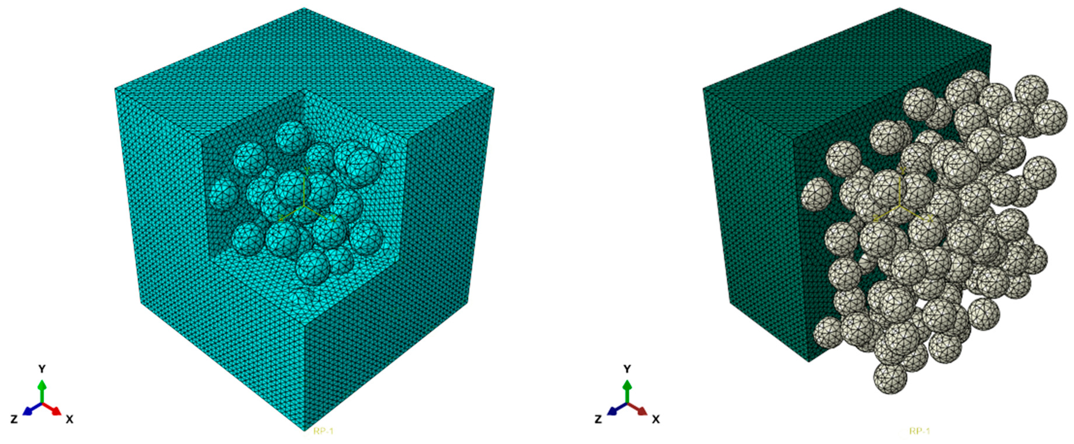
For the successful execution of finite element (FE) simulations, generating a mesh that accurately represents the analyzed system’s geometry is essential. In our study, we employed a free mesh consisting of tetrahedral elements (C3D10) with complete integration to mesh the microstructures, as illustrated in Figure 2. This mesh type is particularly adept at modeling complex geometries, making it an ideal choice for the intricate structures present in our composite material analysis.

To ascertain the minimum number of finite elements needed for accurately meshing an inclusion, we refined the mesh density and monitored the convergence of macroscopic properties. For this purpose, a 3D microstructure containing 200 particles with a volume fraction of 25% was selected as the model system. Throughout the process, various levels of mesh refinement were applied while maintaining the microstructure’s integrity.

The strategy involved increasing the mesh density by reducing the size of the finite elements. Consequently, a greater number of finite elements were utilized to mesh the system. Through this process, we examined the convergence of macroscopic properties to determine the optimal number of finite elements required for precise meshing of a single particle.

In our approach, complete integration was employed utilizing four Gauss integration points per element. This technique facilitated the accurate computation of the microstructure’s macroscopic properties. The use of a free mesh composed of tetrahedral elements enabled effective modeling of the microstructure and a thorough analysis of property convergence.

Accurate mesh generation is fundamental for conducting finite element simulations as it significantly influences the results’ precision. Optimizing mesh density is therefore crucial for the accurate representation of the system. Additionally, studying the convergence of macroscopic properties is essential to establish the ideal number of finite elements for accurate results.

Figure 3, which illustrates the convergence of the bulk modulus and the thermal conductivity in relation to the number of finite elements used for meshing the microstructure, offers crucial insights into determining the optimal mesh density for precise simulations. The figure clearly shows that initially there is a significant decrease in the two moduli as the mesh becomes finer. This trend occurs because finer meshing, involving an increased number of finite elements, leads to a more accurate representation of the microstructure. However, beyond a certain point, as the number of finite elements continues to grow, the bulk modulus reaches a state of stabilization. This observation suggests that beyond this point, further refinement of the mesh does not contribute substantially to the improvement in accuracy.

The convergence analysis revealed that the optimal number of finite elements for achieving accurate results in terms of the bulk modulus is approximately 205,070, while for thermal conductivity, the optimal number is around 180,950. Consequently, we will conduct the calculations using the specifically identified optimal number of finite elements corresponding to the bulk modulus. This figure applies to a volume containing 200 particles, each with a volume fraction of 25%. At this level, the bulk modulus reaches convergence, indicating that further increases in the number of finite elements do not significantly impact the accuracy of the results. Additionally, the analysis shows that the difference in bulk modulus values between simulations using 205,070 and 398,500 elements is less than 1%, reinforcing the notion that further mesh refinement beyond this point does not substantially enhance accuracy.

Consequently, for all subsequent simulations, a mesh density of about 1025 elements per particle was selected. This density effectively balances accuracy with computational efficiency, ensuring precise results while avoiding excessively long simulation durations.

3.2. Boundary Conditions

The process of determining the effective properties of a fictive equivalent homogeneous medium involves solving a boundary value problem within a representative elementary volume $dV$. It is crucial that this volume is adequately sized to capture the complexity of the microstructure inherent in the heterogeneous material. This complexity arises from the presence of various heterogeneities. In the case of periodic distribution of constituents, the required volume is reduced to an elementary cell. This cell can effectively replicate the entire microstructure through simple translation, forming a sort of tiling pattern. Subsequently, this selected volume is subjected to elementary loads or external conditions to obtain a response. This response is then analyzed to derive the effective properties of the composite material. The main challenge of this process lies in the choice of boundary conditions to be applied to the volume under consideration. These boundary conditions [23,27] are crucial to ensure that a given global average strain or stress, i.e., macroscopic, is accurately reproduced in calculations. The idea is basically to model and analyze the material’s behavior on a larger scale, taking into account the collective effects of its microstructure on its overall mechanical response.

3.2.1. Linear Elasticity

In this study, we assume that macroscopic properties are invariant with respect to various boundary conditions. To investigate this, we specifically focus on testing two distinct boundary conditions: the kinematic uniform boundary conditions (KUBC) and the periodic boundary conditions:

-

Kinematic uniform boundary conditions (KUBC): Here, the displacement $\underline{u}$ is imposed at a point $\underline{x}$ on the boundary $\partial V$. The conditions are defined such that:

$$\underline{u}=\underset{\sim }{E}·\underline{x}\forall \underline{x}\in \partial V$$

(5)

Macroscopically, the material is considered isotropic. Hooke’s law is written as follows:

$$\underset{\sim }{\Sigma }=\underset{\underset{\sim }{\sim }}{\left[C\right]}·\underset{\sim }{E}$$

(6)

where:

$\Sigma$: the second-rank macroscopic stress tensor;

E: the second-rank macroscopic strain tensor;

$\left[C\right]$: the fourth-rank macroscopic elastic property tensor of the composite;

${\displaystyle \underset{\sim }{E}}$ is a symmetrical second-rank tensor that does not depend on $\underline{x}$. This implies that:

$$\underset{\sim }{\langle \epsilon \rangle }=\frac{1}{V}{\int }_V\underset{\sim }{\epsilon }\mathrm{d}V=\underset{\sim }{E}$$

(7)

where $<>$ represents the average function and $\epsilon$ is the local strain tensor.

The macroscopic stress tensor is then defined by the spatial average:

$$\underset{\sim }{\Sigma }=\langle \sigma \rangle =\frac{1}{V}{\int }_V\underset{\sim }{\sigma }\mathrm{d}V$$

(8)

where $\sigma$ represents the local stress tensor.

-

Static uniform boundary conditions (SUBC): The traction vector is prescribed at the boundary:

$$\underset{\sim }{\sigma }·\underline{n}=\underset{\sim }{\Sigma }·\underline{n}\forall \underline{x}\in \partial V$$

(9)

where n represents the normal surface vector.

${\displaystyle \sum _{\sim }}$ is a symmetrical second-rank tensor independent of $\underline{x}$. The vector normal to $\partial V$ at $\underline{x}$ is denoted by $\underline{n}$. This implies that:

$$\underset{\sim }{\langle \sigma \rangle }=\frac{1}{V}{\int }_V\underset{\sim }{\sigma }\mathrm{d}V=\underset{\sim }{\Sigma }$$

(10)

The macroscopic strain tensor is then defined as the spatial average:

$$\underset{\sim }{E}=\langle \underset{\sim }{\epsilon }\rangle =\frac{1}{V}{\int }_V\underset{\sim }{\epsilon }\mathrm{d}V$$

(11)

-

Periodicity conditions (PERIODIC): In the context of a periodic structured medium, i.e., one with a repetitive pattern, the elementary volume V is meticulously characterized in terms of its geometric morphologies. The specific shape of this volume is designed in a manner that enables the replication of the entire spatial domain through the simple translational repetition of V. In this study, the objective is to identify a solution field that conforms to a predetermined structure. This sought-after field is expected to capture and reflect the underlying periodicity of the medium. This periodicity is expressed by an equation that can be formulated as follows:

$$\underline{u}=\underset{\sim }{E}·\underline{x}+\underline{v}\forall \underline{x}\in V,$$

(12)

where the fluctuation $\underline{v}$ is periodic. It takes the same values at two homologous points on opposite faces of V. The traction vector $\underset{\sim }{\sigma }·\underline{n}$ takes opposite values at two homologous points on opposite faces of V. The proof of existence and uniqueness of solutions for the three specified boundary value problems advances with a heightened level of scientific rigor, particularly within the linear framework and accounting for potential rigid-body motions or translations. Note that the intricacies of these demonstrations are informed and fortified by results derived from the meticulous averaging computations detailed in the preceding section, as encapsulated by the expressions denoted in Equations (7) and (10). For homogeneous deformation conditions at the edges and periodicity, coupled with dual-stress conditions, a nuanced exploration is necessary. This involves a detailed examination of the interplay between deformation and stress factors, particularly within periodic influences:

$$\langle \underset{\sim }{\epsilon }\rangle =\underset{\sim }{E}$$

(13)

$$\langle \underset{\sim }{\sigma }\rangle =\underset{\sim }{\Sigma }$$

(14)

The averages are performed over the volume V, where uppercase letters (respectively, lowercase letters) denote macroscopic (microscopic) quantities.

In our case, the boundary conditions KUBC, SUBC, and PERIODIC are considered as special cases for which specific values of $\underset{\sim }{E}$ and $\underset{\sim }{\sigma }$ are chosen. To compute effective properties in the case of KUBC and PERIODIC, we choose an elementary volume with imposed macroscopic strain tensors as:

$$\underset{\sim }{E_k}=\left(\begin{array}{ccc}\frac{1}{3}& 0& 0\\ 0& \frac{1}{3}& 0\\ 0& 0& \frac{1}{3}\end{array}\right),\underset{\sim }{E_{\mu }}=\left(\begin{array}{ccc}0& \frac{1}{2}& 0\\ \frac{1}{2}& 0& 0\\ 0& 0& 0\end{array}\right)$$

(15)

An apparent bulk modulus $k^{\mathrm{app}}$ and an apparent shear modulus ${\mu }^{\mathrm{app}}$ can be defined as:

$$\begin{array}{ccc}\hfill & \hfill k^{\mathrm{app}}=\frac{1}{3}trace\underset{\sim }{\langle \sigma \rangle }\mathrm{and}\hfill & \hfill {\mu }^{\mathrm{app}}=〈{\sigma }_{12}〉\end{array}$$

(16)

where: $\sigma$ is the local stress tensor, ${\sigma }_{12}$ is the local shear tensor, and < > represents the average stress on the hole microstructure.

In the case of SUBC, one takes:

$$\underset{\sim }{\Sigma }=\left(\begin{array}{ccc}1& 0& 0\\ 0& 1& 0\\ 0& 0& 1\end{array}\right),{\Sigma }_{\mu }=\left(\begin{array}{ccc}0& 1& 0\\ 1& 0& 0\\ 0& 0& 0\end{array}\right)$$

(17)

In this case an “apparent bulk modulus” $k^{\mathrm{app}}$ and an “apparent shear modulus” ${\mu }^{\mathrm{app}}$ can also be defined as:

$$\frac{1}{k^{\mathrm{app}}}=trace\langle \epsilon \rangle \mathrm{and}\frac{1}{{\mu }^{\mathrm{app}}}=2〈{\epsilon }_{12}〉$$

(18)

3.2.2. Thermal Conductivity

For the thermal problem, the temperature, its gradient, and the heat flux vector are denoted by $T,\nabla T$, and q respectively. The heat flux vector and the temperature gradient are related by Fourier’s law, which reads:

$$\underline{q}=-\lambda \underline{\nabla T}$$

(19)

in the isotropic case. The scalar $\lambda$ is the thermal conductivity coefficient of the considered phase. A volume V of heterogeneous material is considered again. Three types of boundary conditions are used in the study of the effective thermal conductivity:

-

Uniform gradient of temperature at the boundary (UGT):

$$T=\underline{G}·\underline{x}\forall \underline{x}\in \partial V$$

(20)

$\underline{G}$ is a constant vector independent of $\underline{x}$. This implies that:

$$\langle \underline{\nabla T}\rangle =\frac{1}{V}{\int }_V\underline{\nabla T}\mathrm{d}V=\underline{G}$$

(21)

The macroscopic flux vector is defined by the spatial average:

$$\underline{Q}=\langle \underline{q}\rangle =\frac{1}{V}{\int }_V\underline{q}\mathrm{d}V$$

(22)

-

Uniform heat flux at the boundary (UHF):

$$\underline{q}·\underline{n}=\underline{Q}·\underline{x}\forall \underline{x}\in \partial V$$

(23)

$\underline{Q}$ is a constant vector independent of $\underline{x}$. This implies that:

$$\langle \underline{q}\rangle =\frac{1}{V}{\int }_V\underline{q}\mathrm{d}V=\underline{Q}$$

(24)

The macroscopic temperature gradient is given by the spatial average:

$$\underline{G}=\langle \nabla T\rangle =\frac{1}{V}{\int }_V\nabla T\mathrm{d}V$$

(25)

-

Periodic boundary conditions (PERIODIC): the temperature field takes the form

$$T=\underline{G}·\underline{x}+t\forall \underline{x}\in V$$

(26)

Apparent conductivities coincide with the wanted effective properties for sufficiently large volumes V. To evaluate the effective thermal conductivity under both UGT and periodic boundary conditions, the procedure entails defining specific test temperature gradients and fluxes imposed on the elementary volume, outlined as follows:

$$\underline{G}=\left(\begin{array}{c}1\\ 1\\ 1\end{array}\right) \mathrm{and} \underline{Q}=\left(\begin{array}{c}1\\ 1\\ 1\end{array}\right)$$

(27)

They are used respectively to define the following apparent conductivities:

$${\lambda }^{\mathrm{app}}=\frac{1}{3}trace\langle \underline{q}\rangle \mathrm{and}{\lambda }^{\mathrm{app}}=\frac{1}{3}trace\langle \nabla \underline{T}\rangle$$

(28)

After an extensive comparison of results derived from various methods, we decided to employ the periodic method for both linear elasticity and thermal conductivity analyses. This method demonstrated a significant advantage in computation speed while delivering results that were on par with those obtained from other methods.

Beyond its computational efficiency, the periodic method also excels at accurately calculating the elastic properties of complex materials. Its relative simplicity in implementation and its versatility make it suitable for a diverse array of materials and geometries. This combination of speed, accuracy, and ease of application underscores the periodic method’s utility in advanced material analysis.

4. Mathematical Model

Our database comprises 3D microstructures that serve as inputs to provide insight into the elastic and thermal behaviors of materials as outputs. We aim to utilize this database to construct a mathematical model capable of estimating various moduli based on two pivotal parameters: volume fraction and contrast.

The essence of this approach is its ability to predict material properties directly from microstructural data. By employing a database replete with virtual microstructures and correlating this information with the mechanical and thermal properties of materials, we can formulate a model that streamlines and expedites the prediction process.

The forthcoming mathematical model will incorporate the volume fraction and contrast as primary parameters. Volume fraction denotes the proportion of each component within the microstructure, while contrast quantifies the disparity in properties between these components. These parameters are instrumental for determining the macroscopic properties of materials. Our objective is to establish a precise mathematical relationship that links these parameters with the overall properties of the materials.

In the initial phase of our study, we focus on characterizing the material behavior in terms of its volume fraction $V_f$ and contrast C. The objective here is to develop mathematical equations based on finite element calculations tailored for different values of $V_f$ and C that have already been ascertained.

To accomplish this, we employ curve fitting: an optimization technique that involves selecting the most suitable set of parameters for a function so that it aligns well with the observed data trends. Essential to this approach is the defining of a mapping function that links the input data (volume fraction or contrast) to the output data (material properties).

Our goal is to identify parameters for a fundamental function that accurately models the relationship between the material’s behavior and these variables, allowing for flexibility in form. This process will enable us to control the shape of the resulting curve through optimization, pinpointing the precise parameters of the function. In our analysis, we will use a two-dimensional fitting approach, where the x-axis represents the model inputs (either volume fraction or contrast) and the y-axis corresponds to the outputs: namely, the material’s elastic and thermal properties.

To execute curve fitting effectively, we initially define the mathematical form of the objective function and then proceed to identify its parameters that minimize error. This error is quantified as the discrepancy between the output values generated by the proposed mapping function and those derived from finite element calculations. By differentiating this error relative to the function’s parameters, we can ascertain the optimal parameter settings.

Once the parameters have been determined, the mapping function becomes a tool to interpolate or extrapolate new data points within the region of interest. This is achieved by feeding a sequence of input values into the mapping function, which allows us to graphically represent the variation in the output in relation to the input.

For error minimization, we utilize the least squares minimization method [28,29,30]. This method is versatile and applicable to any form of mapping function since all functions can theoretically be expressed in polynomial terms. The use of this method ensures that the best fit for the data is achieved by taking into consideration the least cumulative squared difference between the model and the actual data.

The equation for the error is written in the form:

$$\begin{array}{cc}\hfill E_r& =\sum _{i=1}^n{E}_i^2\hfill \\ \hfill & ={\left(y_1-f\left(x_1\right)\right)}^2+{\left(y_2-f\left(x_2\right)\right)}^2+{\left(y_3-f\left(x_3\right)\right)}^2\dots +{\left(y_n-f\left(x_n\right)\right)}^2\hfill \\ \hfill & =\sum _{i=1}^n{\left(y_i-f\left(x_i\right)\right)}^2\hfill \end{array}$$

(29)

where: n: as the number of data points;

x: input data;

y: output data;

f: mapping function.

Since we want to fit a polynomial, we can write $f\left(x\right)$ as:

$$\begin{array}{cc}\hfill f\left(x\right)& =u_0+u_{1}x+u_2{x}^2+\dots +u_n{x}^n\hfill \\ \hfill & =u_0+\sum _{j=1}^k{u}_j{x}_i^j\hfill \end{array}$$

(30)

where: k is the order of the polynomial.

By replacing f with this expression in the error equation, we obtain:

$$E_r=\sum _{i=1}^n{\left(y_i-\left(u_0+\sum _{j=1}^k{u}_j{x}_i^j\right)\right)}^2$$

(31)

The application of calculus is a well-established method for identifying the minimum of an error function. This involves taking the derivative of the error function with respect to each unknown coefficient, which yields an equation representing the function’s slope. The critical points, where this slope equals zero, are indicative of either a minimum, a maximum, or a saddle point in the function. To pinpoint the minimum, we set the first derivative to zero and solve for the unknown coefficients.

In our case, there are k unknowns, denoted as $a_0,a_1,\dots ,a_k$. The process necessitates computing the derivative for each of these unknowns individually and thereby determining their optimal values to minimize the error function. This approach is crucial for precisely calibrating our model to reflect the actual behavior of the material based on the collected data.

$$\begin{array}{cc}\hfill & \frac{\partial E_r}{\partial u_0}=-2\sum _{i=1}^n\left(y_i-\left(u_0+\sum _{j=1}^k{u}_j{x}_i^j\right)\right)=0\hfill \\ \hfill & \frac{\partial E_r}{\partial u_1}=-2\sum _{i=1}^n\left(y_i-\left(u_0+\sum _{j=1}^k{u}_j{x}_i^j\right)\right)x_i=0\hfill \\ \hfill & \frac{\partial E_r}{\partial u_2}=-2\sum _{i=1}^n\left(y_i-\left(u_0+\sum _{j=1}^k{u}_j{x}_i^j\right)\right)x_i^2=0\hfill \\ \hfill ⋮\\ \hfill & \frac{\partial E_r}{\partial u_k}=-2\sum _{i=1}^n\left(y_i-\left(u_0+\sum _{j=0}^k{u}_j{x}_i^j\right)\right)x_i^k=0\hfill \end{array}$$

(32)

These equations can be re-arranged into matrix form:

$$\left[\begin{array}{ccccc}n& \sum x_i& \sum x_i^2& \cdots & \sum x_i^k\\ \sum x_i& \sum x_i^2& \sum x_i^3& \cdots & \sum x_i^{k+1}\\ \sum x_i^2& \sum x_i^3& \sum x_i^4& \dots & \sum x_i^{k+2}\\ ⋮& ⋮& ⋮& \dots & ⋮\\ \sum x_i^k& \sum x_i^{k+1}& \sum x_i^{k+2}& \dots & \sum x_i^{k+k}\end{array}\right]\left[\begin{array}{c}{u}_0\\ u_1\\ u_2\\ ⋮\\ u_k\end{array}\right]=\left[\begin{array}{c}\sum \left(y_i\right)\\ \sum \left(x_i{y}_i\right)\\ \sum \left(x_i^2{y}_i\right)\\ ⋮\\ \sum \left(x_i^k{y}_i\right)\end{array}\right]$$

(33)

Hence, the solution of the matrix system is:

$$\mathbf{U}={\mathbf{X}}^{-\mathbf{1}}\mathbf{B}$$

(34)

In the end, we can derive the polynomial form that best fits the curve:

$$y=U\left[0\right]+U\left[1\right]x+U\left[2\right]x^2+\dots +U\left[k\right]x^k$$

(35)

The Python library scipy offers an API that is adept at curve fitting to a dataset by identifying optimal parameters for a mapping function. This is achieved through the least squares minimization method, which efficiently finds the best fit for the given data.

4.1. Modeling of Effective Elastic and Thermal Properties of Heterogeneous Material as a Function of Inclusion Volume Fraction

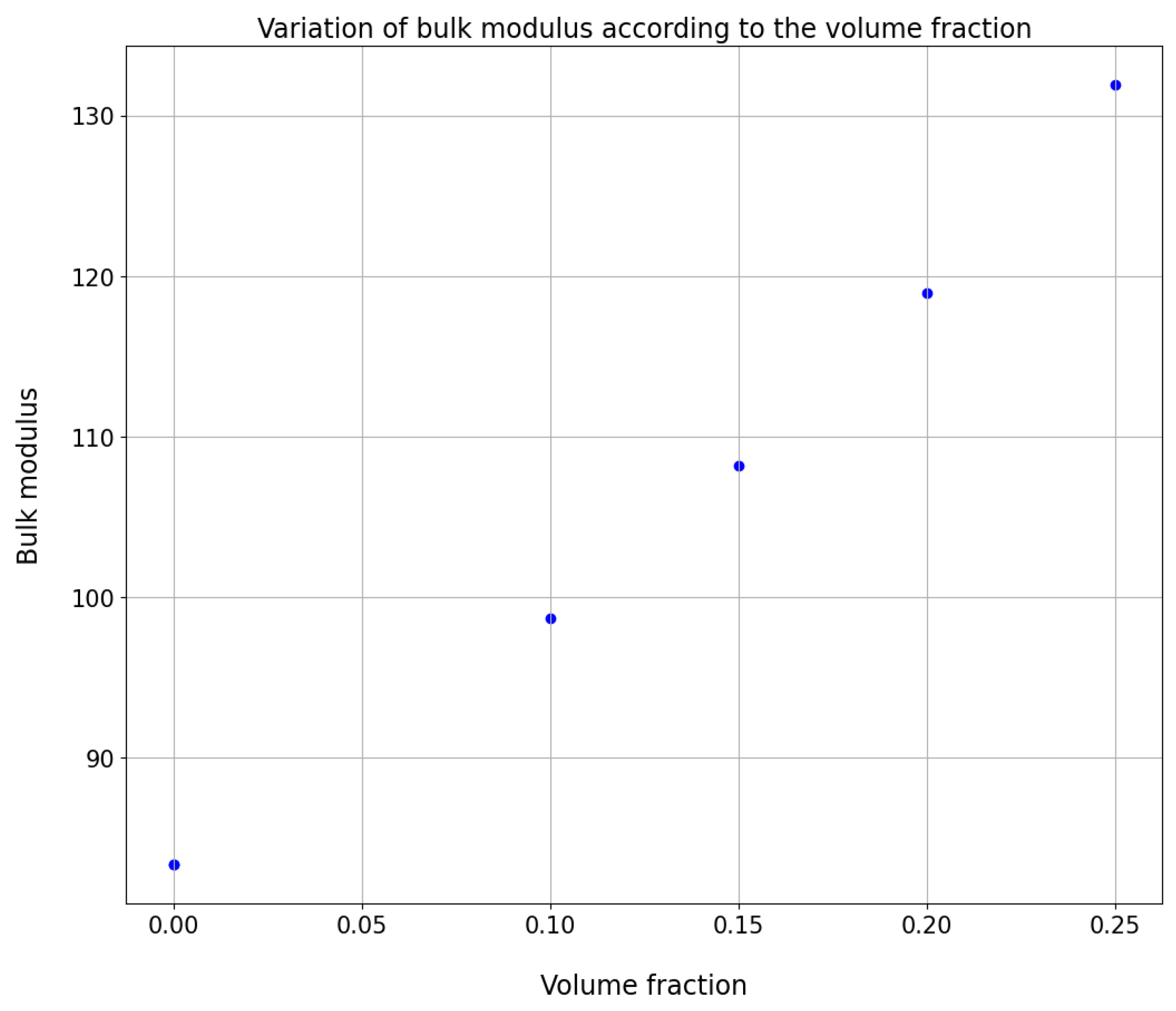
Our initial focus in this study is to analyze how the elastic and thermal behavior of a heterogeneous material varies as a function of the volume fraction while maintaining a constant contrast value.

This investigation entails examining the material’s response to changes to the volume fraction. Volume fraction, in this context, quantifies the proportion of one phase in a two-phase material system. By manipulating the volume fraction and keeping the contrast constant, we gain insights into the dynamic behavior of the material. This approach enables us to identify the ideal volume fraction that results in the desired elastic and thermal properties of the material. Figure 4 visually illustrates the variation in the bulk modulus with different volume fractions.

The selection of appropriate mathematical functions for modeling the intricate relationship between the dependent and independent variables holds paramount significance in data analysis. This becomes especially crucial when confronted with a scatter plot manifesting a nonlinear form: notably, characterized by a discernible parabolic shape in the data points. In delving further into the rationale for this choice, the decision to test both the quadratic polynomial function and the exponential function is based on their distinct abilities to capture and articulate the underlying dynamics between the property of interest and the volume fraction.

Quadratic polynomial function:

$$f_1\left(x\right)=a_0+a_{1}x+a_2{x}^2$$

(36)

where $a_0$, $a_1$ and $a_2$ are adjustable coefficients.

The initial function selected for our analysis is the quadratic polynomial function. This type of function is frequently utilized to characterize physical phenomena demonstrating nonlinear responses. It typically displays an inverted U-shaped curve featuring a vertex at a specific location along the independent variable axis. The quadratic polynomial function is particularly advantageous in modeling scenarios wherein the phenomenon exhibits a peak response at a certain point, followed by a subsequent decrease. Its capability to accurately represent such characteristics makes it an ideal choice for our study’s requirements.

Exponential function:

$$f_2\left(x\right)=\alpha {\mathrm{e}}^{\beta x}$$

(37)

where $\alpha$ and $\beta$ are adjustable coefficients and x is the independent variable.

The second function selected for our analysis is the exponential function, which is frequently employed to represent nonlinear relationships. Depending on the value of the coefficient b, the exponential function can depict either exponential growth or decay. It proves especially effective in modeling scenarios wherein phenomena demonstrate rapid growth or decline and eventually reach a state of long-term saturation.

The choice between polynomial and exponential fitting methods depends on the data’s nature. Polynomial fitting is typically utilized for data exhibiting an overall trend with random fluctuations around it, whereas exponential fitting is more suited for data that show exponential growth or reduction.

Both the exponential and polynomial functions follow a similar operational principle that incorporates three common methods. The first is the least squares method, which aims to find the coefficients $a_0$, $a_1$, and $a_2$ that minimize the sum of the squared differences between the data points and the respective points on the exponential curve or polynomial function. This statistical method is widely used to identify the best-fit line or curve that most accurately represents the data.

The second method is the maximum likelihood method, which seeks to determine the parameter values that maximize the probability of the observed data under the exponential function. This approach is extensively used in probability theory and statistics for parameter estimation for various distributions based on observed data.

The third method employed in our analysis is the nonlinear least squares method: a versatile approach applicable to various nonlinear functions, including both exponential and polynomial types. This method focuses on minimizing the cumulative squared differences between the data points and their corresponding values as predicted by the nonlinear function. Widely utilized in scientific research and engineering, the nonlinear least squares method is integral for optimizing and determining the best-fit model for experimental data.

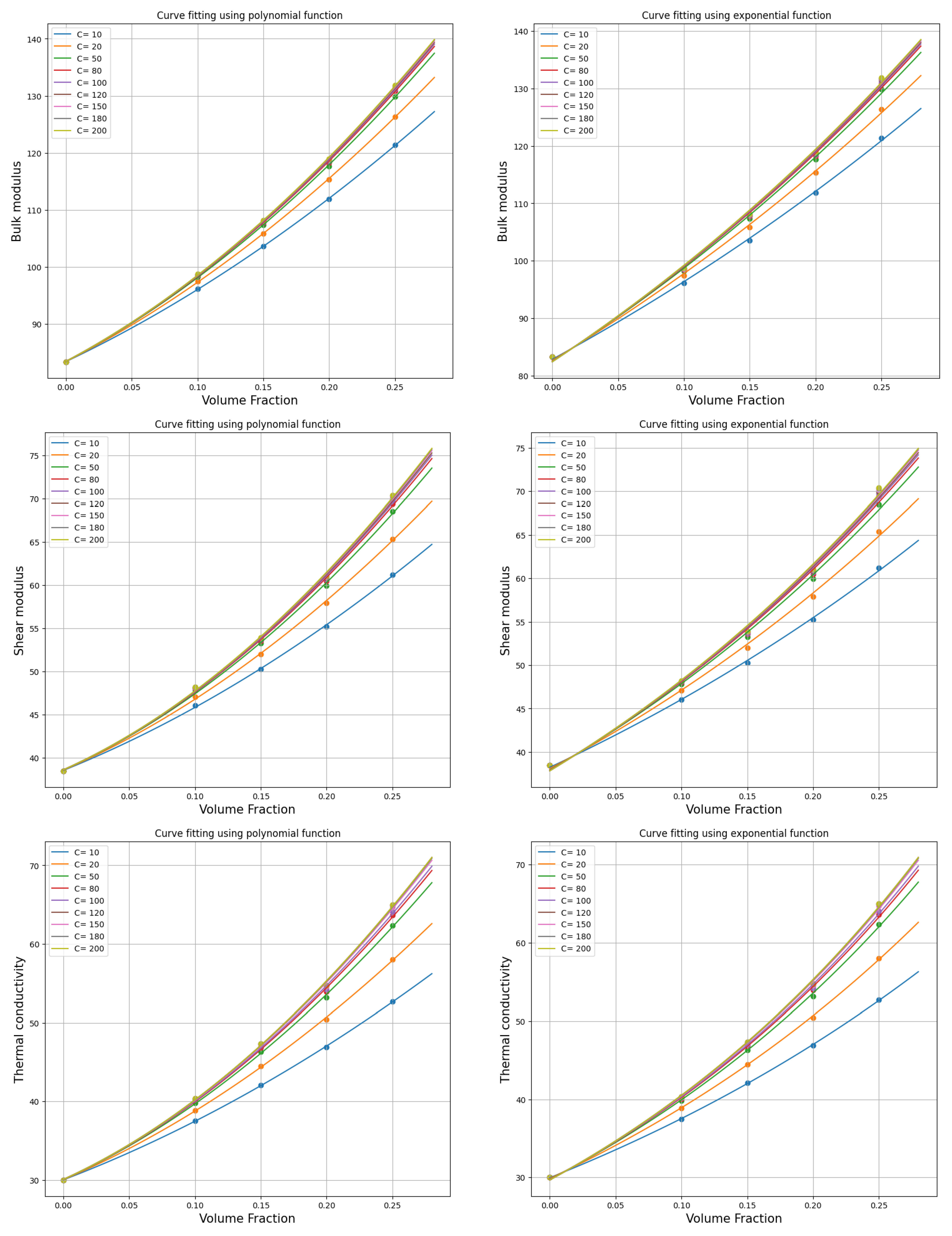
Through the application of these methods—least squares, maximum likelihood, and nonlinear least squares—we are equipped to accurately identify the most suitable model that aligns with our data, be it polynomial or exponential in nature. Figure 5 illustrates the curve-fitting process employing both the polynomial and exponential functions and showcases the versatility and effectiveness of these fitting techniques.

Upon careful analysis of the results derived from the curve-fitting process, we observed that both polynomial and exponential fitting methods yield similar outcomes. However, a critical observation is that the polynomial fitting method aligns more closely with the precise values. This alignment with exact values led us to choose the polynomial fitting method for our analysis. The higher degree of accuracy and precision offered by the polynomial fitting method is instrumental for making well-informed decisions.

Table 2. Optimal coefficients ($a_0$, $a_1$, and $a_2$) of polynomial curve fitting for different contrast values to predict bulk modulus.

Contrast	${\mathit{a}}_0$	${\mathit{a}}_1$	${\mathit{a}}_2$
10	83.354	109.73	167.637
20	83.369	117.306	216.81
50	83.383	121.325	256.56
80	83.38	122.082	268.895
100	83.39	122.344	272.99
120	83.391	122.496	276.023
150	83.39	122.752	278.45
180	83.394	122.857	280.512
200	83.393	122.90	281.484

presents the coefficients $a_0$, $a_1$, and $a_2$ for the polynomial fitting function corresponding to different contrast values. These coefficients’ values change in relation to the contrast, mirroring the variations in material behavior as the contrast increases. An in-depth examination of these coefficients provides valuable insight into the material’s characteristics and how it responds to different contrasts. Utilizing these coefficients in the fitting function enables us to predict the material’s behavior more accurately by substituting the input with a specific volume fraction.

Upon examining the curve and the parameters outlined in the table, a noteworthy observation is made. The formulated equation effectively satisfies the imposed boundary conditions. Notably, when the volume fraction $V_f$ equals zero, the behavior of the material corresponds with that of the matrix phase. This alignment is clearly reflected in the value of $a_0$, which closely approximates the known matrix bulk modulus $K_m$ at 83.33. This congruence demonstrates the equation’s accuracy and reliability at depicting the material’s anticipated response. It also affirms the equation’s capability to precisely represent scenarios for which the dispersed phase’s contribution is minimal or null, reinforcing the model’s validity for diverse material conditions.

4.2. Modeling of Effective Elastic and Thermal Properties of Heterogeneous Material as a Function of the Contrast between Both Phases

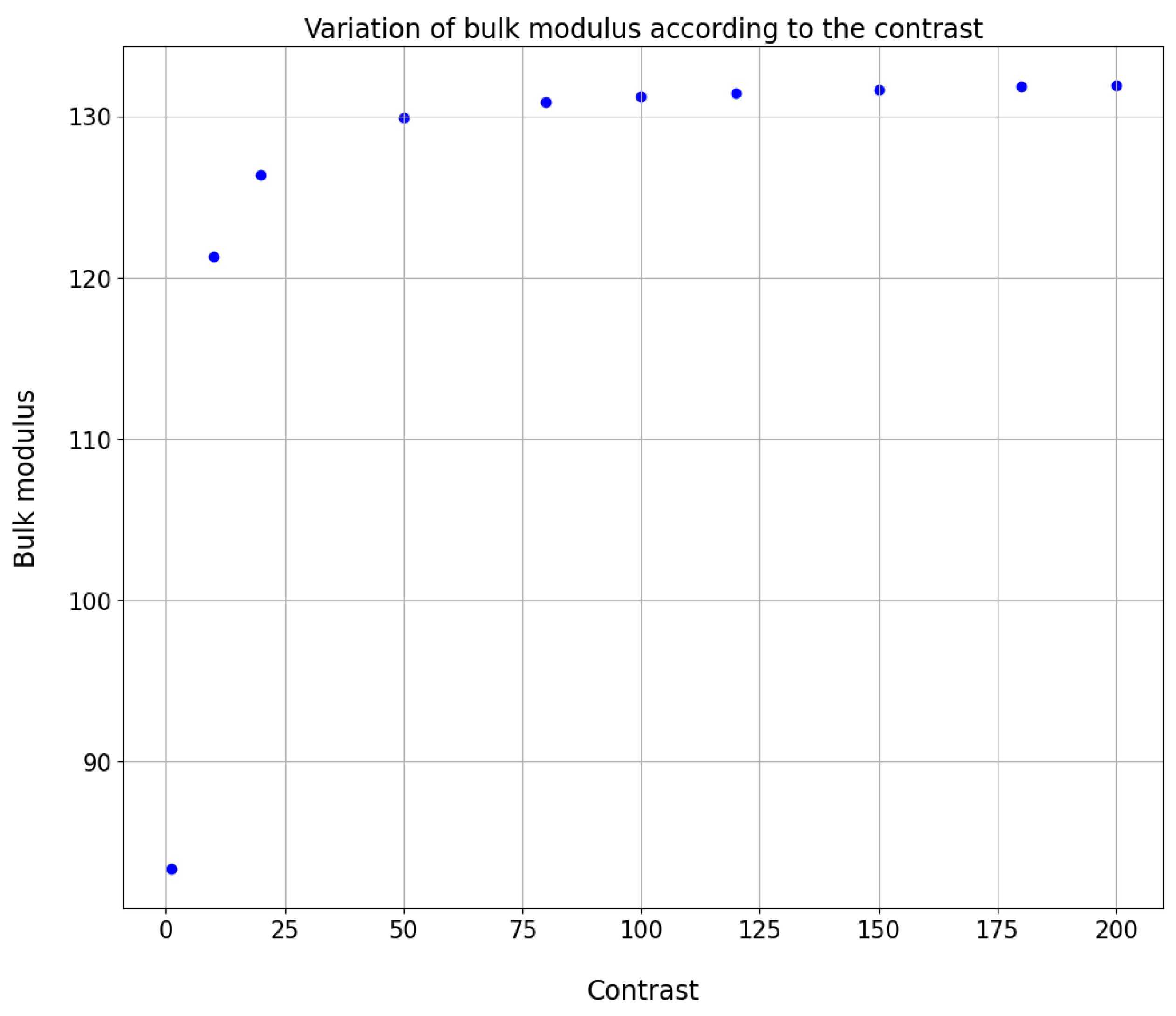
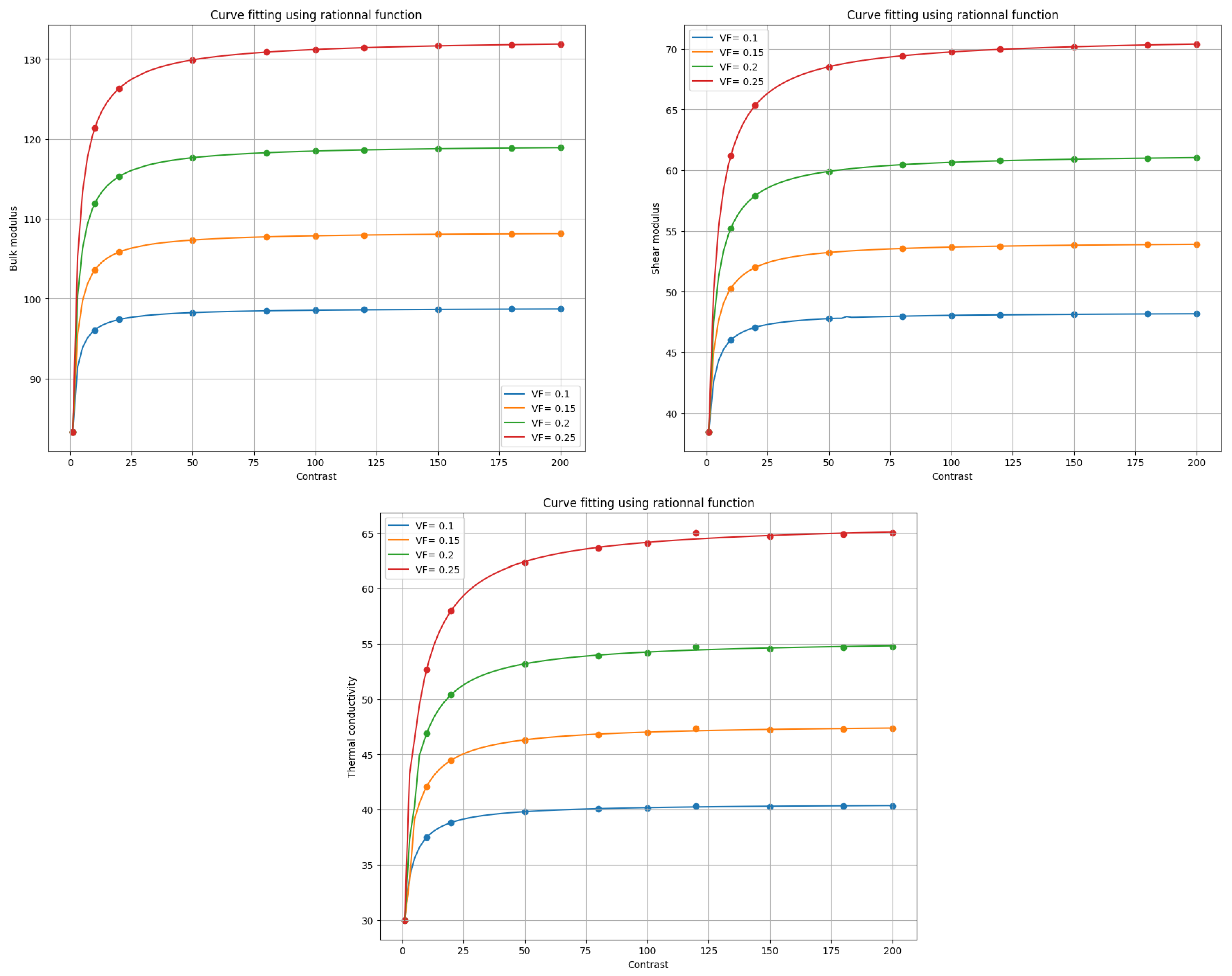
In the second phase of our study, we aim to model the various moduli as functions of contrast by maintaining a constant volumetric fraction. The analysis of the corresponding curve reveals a hyperbolic shape with a horizontal asymptote as the contrast value approaches infinity. This pattern aligns with the anticipated behavior of materials: beyond a certain contrast threshold, the material’s behavior becomes increasingly dominated by the inclusion phase. Essentially, the greater the disparity in properties between the matrix and the inclusion, the more pronounced the influence of the inclusion on the overall properties of the material. This effect is distinctly illustrated by the curve’s shape, which offers insights into the interaction between various parameters and their impact on the material’s properties. Figure 6 visually demonstrates how the bulk modulus varies in response to changes in contrast.

One commonly used mathematical function that can accurately model nonlinear behavior while remaining relatively simple to manipulate and interpret is rational functions. Rational functions are ratios of two polynomials, which gives them great flexibility to adapt to experimental data that may exhibit complex variations. These functions are also well-suited for describing physical phenomena that have asymptotic behavior, meaning they tend towards a limiting value as the independent variable approaches infinity or zero.

$$f\left(x\right)=\frac{b_0+b_{1}x+b_2{x}^2}{c_0+c_{1}x+c_2{x}^2}$$

(38)

where $b_0$, $b_1$, $b_2$, $c_0$, $c_1$, and $c_2$ are adjustable coefficients.

Rational functions stand out for their ability to accommodate data with intricate variations, owing to the flexibility provided by their form. This adaptability arises from the fact that both the numerator and the denominator of a rational function are polynomials, and their coefficients can be adjusted. Such adjustability enables these functions to more precisely fit experimental data compared to other functions with fixed mathematical structures.

Moreover, rational functions are particularly adept at modeling physical phenomena characterized by asymptotic behavior. In these scenarios, as the independent variable trends towards infinity or zero, the function approaches a finite limit, making rational functions suitable for describing such behavior.

Employing rational functions for data fitting allows for a more nuanced representation of the underlying physical or phenomenological principles. The coefficients of the polynomial terms in the function can be interpreted in a physical context, offering deeper insights into the system’s behavior.

To determine the optimal coefficients $b_i$ and $c_i$ for the rational function, least squares regression analysis is commonly used. This involves minimizing the sum of the squares of the differences between the observed data points and the values produced by the function. By taking partial derivatives of the error function $E_r$ with respect to each coefficient and setting them to zero, we obtain a system of linear equations. Solving these equations yields the coefficients that minimize $E_r$.

Techniques such as matrix algebra or Gaussian elimination can be utilized to solve this system of linear equations. With the optimal coefficients determined, the rational function can then be used to predict dependent variable values for any given independent variable within the data range. By comparing these predictions to the actual data, the fit’s accuracy can be assessed, and adjustments to the coefficients can be made as necessary.

Figure 7 illustrates the fitting of various moduli using the quadratic rational function. These curves visually demonstrate how the values of the moduli vary with the parameter and help to establish the relationships between contrast and material properties.

Table 3. Optimal coefficients ($b_i$ and $c_i$) of rational curve fitting for different volume fraction values to predict bulk modulus.

Volume Fraction	${\mathit{a}}_0$	${\mathit{b}}_1$	${\mathit{b}}_2$	${\mathit{c}}_0$	${\mathit{c}}_1$	${\mathit{c}}_2$
10%	1046.42	1245.90	5.009	14.512	12.618	0.050
15%	1175.60	1271.47	−2.202	16.843	11.716	−0.020
20%	−311.25	−282.73 5	2.722	−4.378	−2.352	0.022
25%	−6775.65	−4450.62	178.847	−88.797	−32.136	1.349

presents the coefficients $b_i$ and $c_i$ for the fitting functions associated with different volume fraction values. These coefficients exhibit variations depending on the volume fraction, indicating changes in the material behavior as the volume fraction increases. Analyzing these coefficients provides valuable insights into the characteristics of the material and its response to the volume fraction. By utilizing these coefficients obtained from the fitting function, one can predict the material’s behavior by substituting the input value with a desired contrast.

An intriguing observation arises from analysis of the curve and parameter table. It becomes apparent that the preceding equation successfully satisfies the imposed boundary condition. Specifically, when the contrast value is set to 1 (C = 1), the material’s behavior aligns with that of the matrix phase. This correlation is clearly manifested in the calculated value of ($b_0$ + $b_1$ + $b_2$)/($c_0$ + $c_1$ + $c_2$), which closely approximates the known value of $K_m$ (matrix bulk modulus) at 83.33. This result effectively demonstrates the equation’s accuracy and reliability for capturing the anticipated material response and validates its ability to faithfully represent the scenario for which the dispersed phase becomes negligible.

4.3. The Analytical Bounds

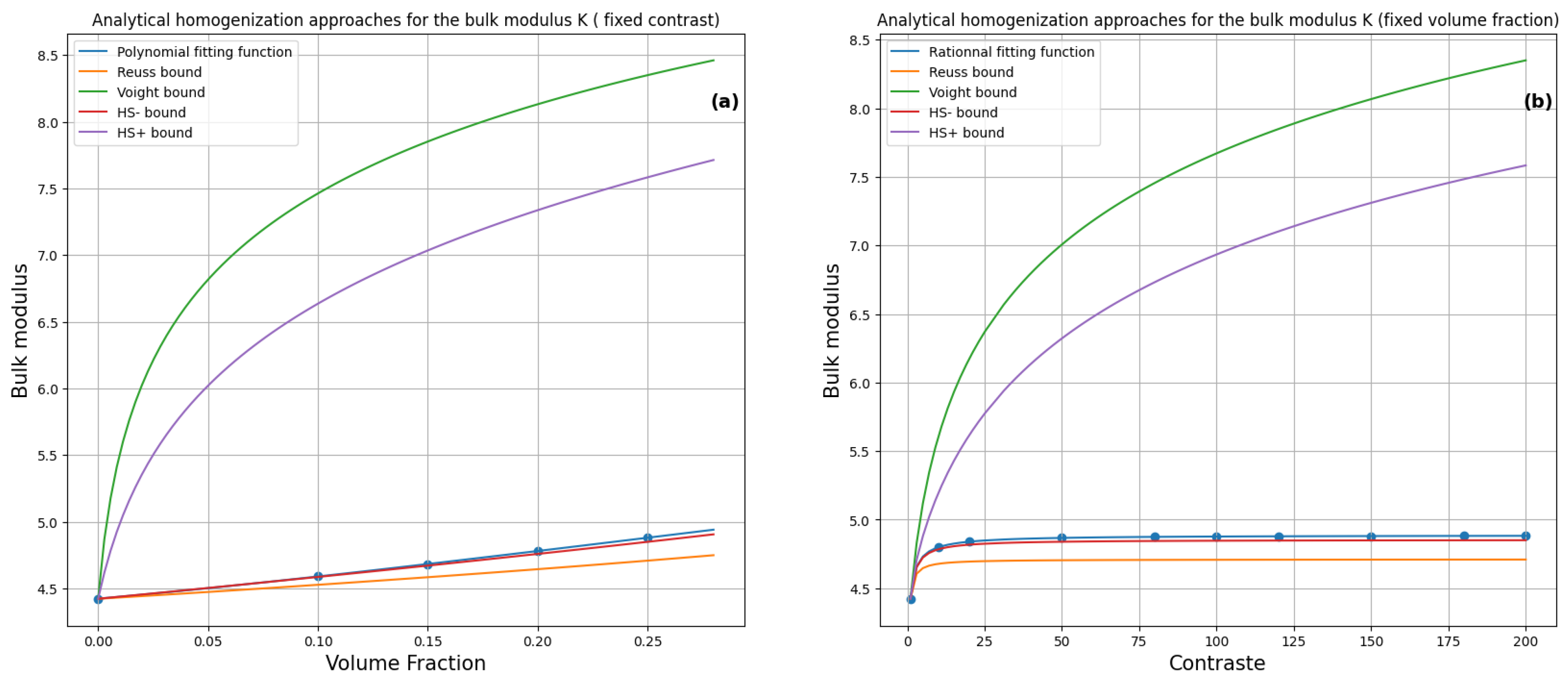
When analyzing numerical data and utilizing fitting functions to model relationships between various measured variables, it is imperative to ensure that the results align with theoretical expectations and bear physical significance. The first- and second-order analytical bounds offer theoretical limitations for the properties of composite materials relative to the volume fraction of each component. These bounds are instrumental for validating fitting functions and enhancing the credibility of experimental data analyses.

The first-order bounds, known as the Voigt–Reuss bounds, provide foundational limits. The Voigt bound is derived under the assumption that all phases are elastically isotropic and results in the application of the Voigt mixing rule for the overall elastic property calculation. Conversely, the Reuss bound is based on the same isotropy assumption but employs the Reuss mixing rule.

Moving to the second-order bounds, known as the Hashin–Shtrikman bounds, we find the upper bound (HS+) and lower bound (HS−). The HS+ bound is established assuming rigidly connected inclusions using the Hashin–Shtrikman mixing rule and is particularly relevant for fiber-reinforced or ceramic matrix composites. The HS− bound, meanwhile, assumes completely isolated inclusions and also employs the Hashin–Shtrikman mixing rule.

To validate the outcomes derived from fitting functions, it is critical to juxtapose the fitting curves with these analytical bounds. If the curves reside within the established first- and second-order bounds, it signifies consistency with theoretical principles and affirms that the fitting function yields physically meaningful parameters. Conversely, curves lying outside these bounds may suggest issues with the fitting function or discrepancies with theoretical assumptions.

In Figure 8, we have plotted the bulk modulus of a composite material with a high contrast ratio of 200 as a function of volume fraction. Additionally, we have plotted the same modulus as a function of contrast ratio for a fixed volume fraction of 25%. In both plots, we have included the Voigt–Reuss bounds and Hashin–Shtrikman bounds of order 1 and 2 for comparison.

To better visualize the behavior of these bounds, we have applied a logarithmic scale to the y-axis.

The fitting curves derived from the graphs clearly demonstrate that the effective properties of the material are accurately captured by the selected functions. The alignment of these curves within the first- and second-order Voigt–Reuss and Hashin–Shtrikman bounds is a testament to the precision of our fitting results. This not only validates the fitting process but also reinforces the reliability of the homogenization methods employed for analyzing the properties of composite materials.

The implications of these accurate fitting results extend into the realms of design and engineering of composite materials. Precise characterization of material properties enables more accurate predictions of composite material behavior under various load conditions, facilitating optimized design processes.

In conclusion, the successful fitting of material property curves using second-degree polynomial and rational functions, coupled with their compliance with the Voigt–Reuss and Hashin–Shtrikman bounds of order 1 and 2, unequivocally validates the efficacy of this novel approach for the analysis of heterogeneous materials. This alignment not only underscores the accuracy of the method but also highlights its potential for broad applications in material science and engineering.

4.4. Generalized Model

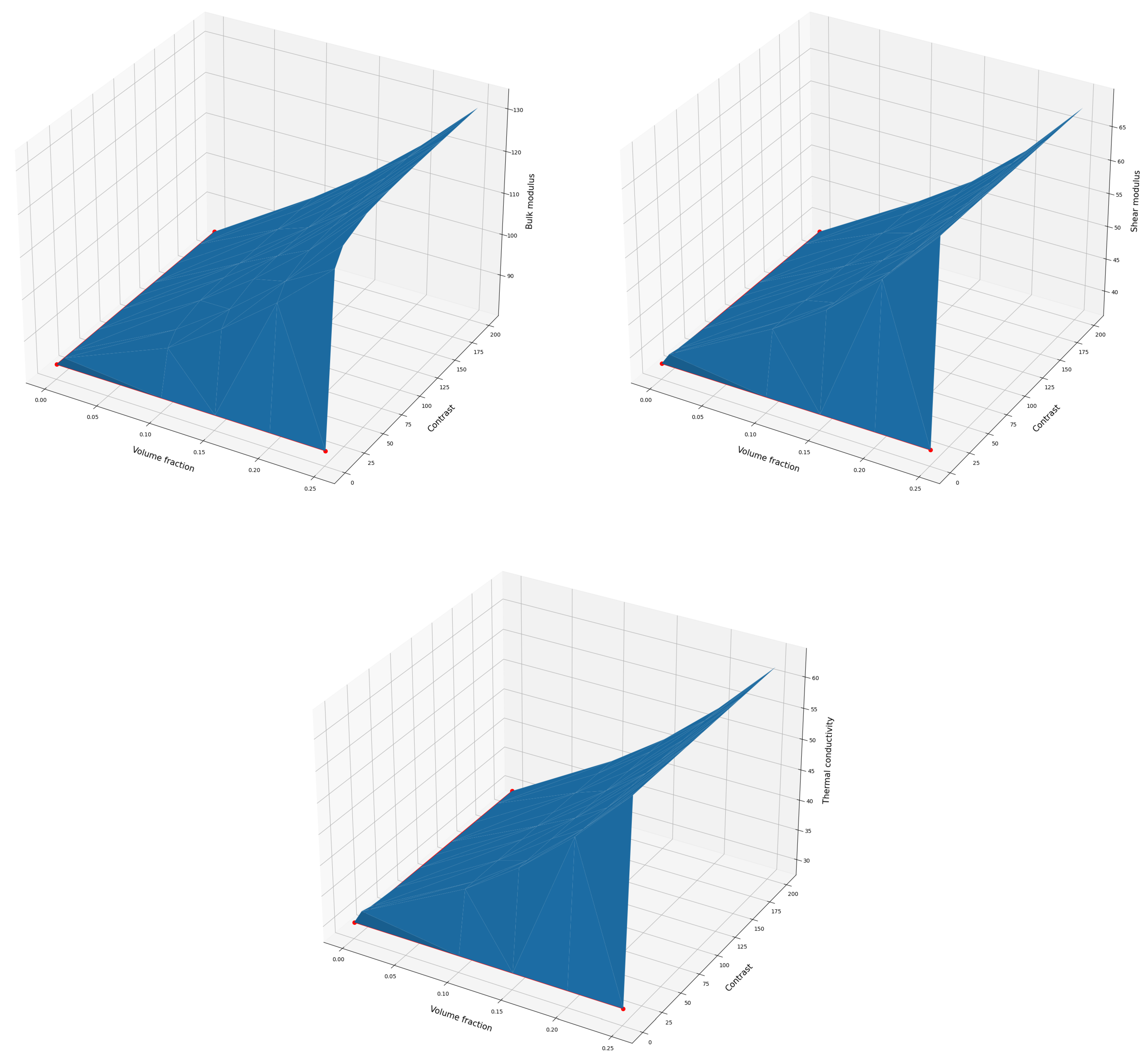
Integrating both the polynomial and rational functions into a unified model that incorporates the volume fraction and contrast as inputs significantly enhances our ability to model the intricate behavior of composite materials. The polynomial function is adept at tracing the general trend of material behavior as the volume fraction varies, whereas the rational function is more effective at capturing the changes to behavior as the contrast between the constituents of the composite material increases.

Moreover, this combined approach allows for a more thorough consideration of the interplay between volume fraction and contrast. For instance, an increase in the volume fraction could intensify the interaction between the composite’s constituents, potentially leading to a nonlinear relationship between behavior and contrast.

By employing both polynomial and rational functions, we can adeptly represent both the overarching trends and the subtle, complex interactions between these two key variables. This dual-function approach culminates in a more precise and comprehensive model of the composite material’s behavior. The final integrated function, which embodies this dual approach, is formulated as follows:

$$f(x,y)=(a{x}^2+bx+c)\left(\frac{d{y}^2+ey+f}{g{y}^2+hy+k}\right)$$

(39)

where:

x, y respectively represent the volume fraction and the contrast;

a, b, c, d, e, f, g, h, and k are adjustable coefficients.

Figure 9 shows a 3D curve constructed using the function that represents the product of the polynomial function and the rational function in two variables: volume fraction and contrast. This function was developed to describe the behavior of composite materials as a function of these two parameters.

The 3D curve generated in our study vividly illustrates the evolution of material properties in response to variations to the volume fraction and contrast. On this curve, the axes represent the two independent variables—volume fraction and contrast—while the surface of the curve maps the dependent variable, which in this case is the material properties.

Significantly, the two red lines on the curve demarcate the boundary conditions where the volume fraction $V_f$ equals zero and the contrast C is one. These lines mark the extreme limits of our study and highlight scenarios where the dispersed phase’s volume fraction is nil and the contrast is at its minimum, which perfectly aligns with the matrix phase.

Close examination of the 3D curve reveals regions where the material properties reach their highest and lowest points as functions of volume fraction and contrast. It also illustrates the global evolution of material properties when one parameter remains constant while the other varies. Consequently, this curve enhances our understanding of the interrelationships between parameters and properties in composite materials and offers valuable insights for the design and manufacturing of optimized composites.

Table 4. The optimal coefficients of the generalized fitting function obtained for the bulk modulus, shear modulus, and thermal conductivity.

Coefficient	a	b	c	d	e	f	g	h	k
Bulk	229.9	108.3	66.35	242.6	−5268.4	7370.9	11.69	−220.2	−324.07
Shear	182.75	60.65	20.71	−142.5	2905.9	−817.47	−6.94	123.02	334.16
Thermal	194.1	66.68	14.27	−103.91	5525.81	−3917.67	−5.44	265.67	1049.5

presents the optimal values of the coefficients for the resulting function that most effectively fit the curve; these values encapsulate the nuanced relationships.

5. Conclusions

In this article, we introduced a novel homogenization method centered around curve-fitting techniques. This method presents notable advantages in terms of time and resource efficiency, particularly when compared to conventional numerical or analytical methods. The development of our model comprised several key stages.

Initially, we collected 3D microstructures featuring 200 spherical inclusions while varying the contrast between the phases and their volume fractions. Employing finite element homogenization, we calculated various moduli, including the bulk modulus, shear modulus, and thermal conductivity. The resultant database was then leveraged to construct a mathematical model through a three-step process. The first step involved plotting module curves as functions of the volume fraction and contrast and enabled us to ascertain the shapes and limits of each curve and gain insight into the behavior of the modules. Subsequently, in the second step, we mathematically synthesized and integrated these modules to create a unified model that accurately predicts the values of different moduli. This involved analyzing the interrelations between the modules and the specific parameters to identify patterns and trends. Finally, we formulated mathematical equations or functions that effectively encapsulate and represent these relationships.

This methodical development process culminated in a robust mathematical model capable of precisely predicting different moduli based on variations to the volume fraction and contrast. The model offers a comprehensive understanding of the interplay between these parameters and the modules and thus serves as an invaluable tool for efficient and accurate predictions for similar heterogeneous material systems.

The results obtained affirm the efficacy of the chosen mapping functions and parameters. The functions are in compliance with the imposed boundary conditions and align with the first- and second-order analytical bounds. This alignment underscores the model’s success at capturing the fundamental characteristics and behaviors of the modules in question and validates its application in the field of material science and engineering.