Abstract
Heat switches are devices for controlling heat flow in various applications, such as electronic devices, cryogenic cooling systems, spacecraft, and rockets. These devices require non-linear transient thermal simulations, in which there is a lack of information. In this study, we introduce an innovative 1D thermo-hydraulic lumped parameter model to simulate loop heat pipes as heat switches by regulating the temperature difference between the evaporator and the compensation chamber. The developed thermo-hydraulic model uses the continuity, energy, and momentum equations to represent the behaviour of loop heat pipes as heat switches. The model also highlights the importance of some thermal conductance parameters and correction coefficients for accurately simulating the different operational states of a loop heat pipe. The simulations are conducted using the proposed 1D model, solved through the application of the Mathcad block function. The numerical model presented is successfully validated by comparing the temperatures of the evaporator and condenser inlet nodes with those of a referenced loop heat pipe from the literature. In conclusion, in this research, the mathematical modelling of loop heat pipes as heat switches is presented. This is achieved by incorporating correction coefficients with Boolean logic that results in non-linear transient simulations. The presented 1D thermo-hydraulic lumped parameter model serves as a valuable tool for thermal system design, particularly for systems with non-linear operational modes like sorption compressors. The graphical and nodal representation of this proposed 1D thermo-hydraulic model further enhances its utility in understanding and optimising loop heat pipes as heat switches across various thermal management scenarios.
1. Introduction
Heat pipes are highly efficient heat transfer devices, functioning on the principles of fluid phase transition and thermal conduction. They come in various geometries and sizes, typically in the form of sealed tubular devices filled with a specific type and amount of working fluid. The fluid undergoes vaporisation at the evaporator section, which is in contact with a heat source. Using the pressure generated by temperature differences, the vapour travels to the condenser, where it releases its latent heat to a cold source. The fluid then condenses back into liquid form and is passively pumped by the Wick structure back to the evaporator through capillary action. This combination of liquid and vapour phases enables extremely efficient heat transfer. Since heat pipes are closed-circuit systems, they operate continuously.
Heat pipes exhibit non-linear performance and require modelling encompassing heat transfer, fluid flow, and thermodynamics. These devices find wide applications in the aerospace industry, whether as individual heat pipes [1], pulse oscillating heat pipes [2], or loop heat pipes [3,4]. The advantage of loop heat pipes over standard heat pipes lies in their ability to dissipate substantial heat power over long distances without any loss in performance.
Heat switches (HS) are devices designed to regulate heat conduction within specific temperature ranges, typically from 0.05 K to nearly 400 K [5]. Heat switch technology finds important applications in “vibration-free” sorption compressors used in cryogenic Joule–Thompson coolers [5]. These advanced cooling systems are employed in space and ground scientific missions, such as Planck [6], Metis [7], and other Earth observation infrared missions [8,9,10]. The incorporation of heat switches in these systems ensures reliable performance by eliminating disruptive vibrations, leading to enhanced accuracy and precision in scientific measurements. Among the various heat switch technologies, the gas-gap heat switch (GGHS) [5,8,11,12,13,14,15,16,17,18,19] is most commonly used.
A recent developed sorption compressor system, part of the vibration-free cryogenic cooler project at Nova University (Portugal), as referenced in [9,10], has implemented a gas-gap heat switch that did not meet performance expectations. Unexpectedly long periods of both cooling and heating were observed due to higher thermal conductance in the elements between the sorption cell and the cooling source. This discrepancy is likely attributed to the OFF state of the gas-gap heat switch, which is almost three times higher than expected [10]. The design requirements for this cryogenic cooler unit included maintaining an evaporator temperature (cold tip) at 80 K, achieving a cooling power between 1 W and 1.5 W and fitting the system within a volume of 0.2 m. The cooler system comprises four adsorption cells, each containing 600 m of active medium made of HKUST-1, and a set of valves that regulate gas flow. After the compressed refrigerant gas exits the compression unit, it undergoes cooling through the heat exchanger. Subsequently, during its expansion through a Joule–Thomson valve, the refrigerant absorbs heat from the device being cooled. The adsorption cells of the compressor operate within the temperature range of 150 K to 400 K. Electric heaters and heat sinks are employed for heating and cooling the cells, respectively. Heat switches are used to establish thermal contact between these heated sorption cells and the heat sink (cold plate at 150 K). The OFF state of the switch is activated when heating the cell for gas desorption (compression), while the ON state is employed when the aim is gas adsorption during expansion, allowing heat dissipation into the cold source (heat sink). The malfunctioning gas-gap heat switch has been identified as a contributing factor, leading to undesired extended cycle duration and increased heating power requirements for the sorption cell.
A loop heat pipe presents promising alternative heat switch solutions in this sorption compressor application. This functionality is achieved by enabling the control of the temperature differential between the evaporator and the compensation chamber, as described in [20,21]. To implement it, a 1D thermo-hydraulic lumped parameter model mathematical model, as in [22,23,24,25,26,27,28,29,30], capable of predicting design and thermal performance, is necessary. This model should account for transient responses, complex interactions involving two-phase fluid flow, heat transfer, flow through porous structures, dry-out and priming phenomena, as well as condensation and evaporation within the loop heat pipe.
This article’s objective is to introduce an analytical 1D thermo-hydraulic mathematical model, offering a comprehensive understanding of the non-linear behaviour and thermal performance of loop heat pipes when functioning as heat switches. Currently, there is a lack of mathematical modelling references to address how the loop heat-pipe responds thermally in transient simulations, considering various state modes, such as a de-primed wick. By considering the intricate dynamics of two-phase fluid flow, heat transfer, and various phenomena, our objective is to provide valuable insights for the design and optimization of loop heat pipes as heat switches, particularly for sorption compressors in systems used for space applications.
The innovation of this article lies in its demonstration of how a lumped parameter model of a loop heat pipe can be effectively configured to illustrate its non-linear behaviour, resembling that of a heat switch. This non-linearity is a distinguishing feature due to the loop heat pipe having five (5) distinct operational states. These valuable insights will significantly contribute to improving the efficiency and performance of various engineering applications that require a transient simulation and cannot be analysed by a steady-state approach.
This paper, which aims to develop a 1D thermo-hydraulic lumped parameter model [22,23,24,25,26,27,28,29,30] for a loop heat pipe working as a heat switch, is organized as follows: Section 2 presents the mathematical model of the loop heat pipe working as a heat switch, Section 3 focuses on the dimensioning parameters, such as geometry and fluid properties, which are used in the simulations, and the corresponding results are presented in Section 4. Section 5 involves a discussion on the challenges and achievements from the prop- osed model.
2. Modelling
The geometrical configuration of the loop heat pipe used for the proposed mathematical model is based on Figure 1. It comprises a heat source (Node 8), a vapour transport line (Nodes 2 to 3), a liquid transport line (Nodes 5 to 6), a condenser (Nodes 3, 4 and 5), compensation chamber liquid (Nodes 6 to 7) and an evaporator (Node 1).
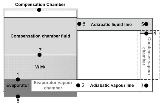
Figure 1.
Loop heat pipe generic configuration.
In this model, the loop heat pipe is analysed as a system of nodes and control volumes, , as shown in Figure 2 and Figure 3. Nodes are used to represent the solid elements, and control volumes are assigned to represent a specific mass of liquid or vapour that exists on each section. For example, between Node 1 (evaporator entrance) and Node 2 (evaporator exit) there is control volume , which defines the contained mass in a vapour state within the evaporator vapour chamber. This logic is applied to the remaining nodes and control volumes.
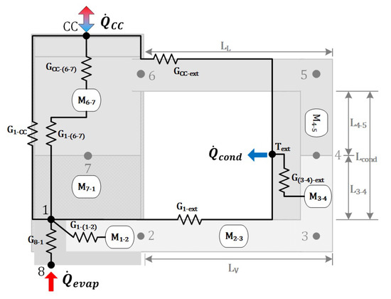
Figure 2.
Equivalent thermal network with nodes and control volumes.
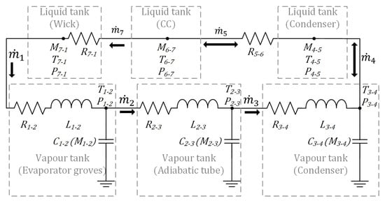
Figure 3.
Equivalent hydraulic network with nodes and control volumes.
With these nodes and control volumes, we define a thermo-hydraulic model that can be represented as in Figure 2 and Figure 3 using resistive, capacitive, and inductive elements.
By defining the boundary conditions at the evaporator, compensation Chamber and external temperature nodes, i.e., , and , respectively, a 1D model represented by a set of Ordinary Differential Equations (ODEs) can be obtained. The results of these equations allow for a comprehensive understanding of the transient thermo-hydraulic behaviour of the loop heat pipe when operating as a heat switch.
The circuit elements presented in Figure 2 and Figure 3, the thermal and hydraulic network systems, respectively, are based on equivalent electrical circuit elements such as Resistive R, Capacitive C and Inductive L. For clarity and consistency within this article, symbol G is used to represent thermal conductance, deviating from conventional symbol used for thermal resistance, given that . This decision was made to avoid confusion with the use of in the hydraulic model, as previously described.
2.1. Thermal Network Model
The loop heat pipe thermal network consists of two distinct elements: thermal conductance (G) and thermal capacitance (). Thermal conductance can be either axial or emphradial as shown in (1) and (2):
where A is the cross-sectional area through which heat transfer occurs, k is the material thermal conductivity, L is length, and and are the outside and inside diameters, respectively, for the case of the evaporator being a radial element. The thermal conductance values shown in Figure 2, based on the previous assumptions, are as follows:
- : Represents the thermal conductance between Node 8 and Node 1 relative to the heat source and evaporator, respectively.
- : Represents the thermal conductance between Node 1 and the compensation chamber node.
- : Represents the thermal conductance between Node 1 and the external node, relative to the evaporator and the external environment temperature node. This includes the transport pipeline for the liquid phase.
- : Represents the thermal conductance between the compensation chamber node and the external environment temperature node. This includes the transport pipeline for the vapour phase.
The thermal conductance associated with convection between fluids and surfaces, i.e., and , is as in (3):
where h is the convective heat transfer coefficient of liquid or vapour, and is the contact surface area between the fluids. The h coefficient is an empirical value usually obtained through thermal tests.
Finally, we can address the last two thermal conductances that are associated with the Wick and evaporator components, i.e., and , respectively. In both Gs, it is necessary to understand whether the loop heat pipe is an axial (1) or radial (2) design, and also include convective coefficient h (3) every time there is a thermal contact between fluid and solid. However, a different approach is required for the Wick effective thermal conductivity, , as shown in [31]:
In (4), is the solid material thermal conductivity, is the thermal conductivity of the working fluid in a liquid phase, and represents Wick porosity. The thermal capacitances () considered for the thermal network from Figure 1 are
- : Represents the thermal capacitance of evaporator saddle.
- : Represents the thermal capacitance of evaporator grooves that are in contact with the Wick.
- : Represents the thermal capacitance of compensation chamber cannister.
- : Represents the thermal capacitance of fluid inside the compensation chamber.
These thermal capacitances are then evaluated by
where M is the mass, V is the volume of the given node, is material density and is material heat capacitance of the associated node. Similarly, in Wick thermal conductance, there is also an effective thermal capacity to be estimated:
The general transient heat conduction equation governing each solid node (, , , ) is given by
where is the temperature of node i, is the temperature of adjacent node j, and is the thermal conductance between i and j.
2.2. Hydraulic Network Model
Modelling fluid processes pose significant challenges in this study. To overcome this challenge, first, it is necessary to understand the fundamentals of the elements used in the hydraulic network; Figure 3. The modelling of fluid processes necessitates the use of three elements, including fluid storage Capacitance, , used to estimate the pressure variation in due to ; and since the vapour phase is compressible, i.e., , it results in
where is vapour tank volume, is vapour adiabatic index, is specific gas constant and is vapour temperature.
Flow inductance L is used to estimate the “quantity of motion”, , and it is therefore expressed as
where is the effective length of the pipe at vapour tank exit, and is the hydraulic area of the transport lines.
Lastly, we have the fluidic resistance, , that is obtained from Hagen–Poiseuille and the Darcy equation:
where is the effective length of the pipe at vapour tank exit, is the vapour dynamic viscosity, is the vapour density, is the hydraulic area, and is the internal radius of the transport lines.
The foregoing three basic elements, , and , are used in the governing equations of energy, momentum and continuity in order to construct an equivalent hydraulic network as illustrated in Figure 3. For the hydraulic network, several fundamental assumptions are to be considered:
Assumption 1.
Fluid path is considered one-dimensional.
Assumption 2.
The liquid phase is assumed to be incompressible.
Assumption 3.
The vapour phase is represented using ideal gas equations.
Assumption 4.
Vapour temperature and pressure variation are derived from the Clausius–Clapeyron equation.
Assumption 5.
The flow is assumed to be laminar for both vapour and liquid phases.
Assumption 6.
Evaporation and condensation phenomena are confined to the evaporator and condenser zones, respectively.
Assumption 7.
The temperature of liquid present in the Wick section of the heat pipe is assumed to be equal to the temperature of the Wick in that region.
The liquid and the vapour are divided into two different regions, i.e., liquid tanks and vapour tanks, respectively, as shown in Figure 3. For the vapour, we have three tanks corresponding to the vapour storage in the evaporator grooves, the adiabatic tube and the condenser. There are two vapour paths corresponding to the flow through the vapour tanks. Similarly, three liquid tanks and two liquid paths are assumed for the liquid region. The liquid region and vapour region are connected by two additional paths, which represent evaporation and condensation, using latent heat expression . The fluid cycle, represented in Figure 2 and Figure 3, can be summarized in six steps:
- Step 1
- The evaporator, Node 1, is heated up and the liquid tank produces vapour; a mass of vapour is produced and flows into vapour tank .
- Step 2
- Pressure, , increases inside vapour tank and the mass of vapour, , is pushed into vapour tank , i.e., representing the adiabatic vapour tube pipe.
- Step 3
- Pressure, , increases inside the vapour tank and the mass of vapour, , is pushed into the vapour tank , i.e., representing vapour on the condenser tube.
- Step 4
- The condenser (Node 4) cools down and a mass of fluid is condensed and flows into condenser liquid tank .
- Step 5
- The condensed liquid pushes a mass of liquid from condenser liquid tank through the tube pipe, i.e., from Node 5 to Node 6, leaving the tube with a mass of liquid into compensation chamber tank .
- Step 6
- The liquid entering compensation chamber tank pressure-pushes a mass of liquid again to Wick tank , thus completing the fluid loop.
In the upcoming sections, we develop the energy, momentum, and continuity equations that are specific to each fluidic element. Separate equations are derived for the vapour and liquid phases to account for their distinct behaviours.
2.2.1. Vapour Equations
Vapour masses (, and ) are modelled as an ideal gas (as in Assumption 3), which means that continuity equation applied to the three vapour masses is rewritten as follows:
where is the mass flow rate, P is the pressure, is the universal gas constant, t is time, V is the tank volume, T is the temperature of the vapour in the tank, is the atomic weight, and is the flow capacitance. The temperature time derivative, , of the adiabatic vapour masses M is modelled according to the Clausius–Clapeyron relation, , as discussed in [32], providing a link between vapour pressure P and temperature T:
Following Assumptions 1 and 5, the 1D momentum equations for the vapour flow through the vapour ducts are as follows:
Integrating Equation (17) for each section in the evaporator and adiabatic pipe effective lengths, i.e., and , respectively, we obtain
Assuming that we have constant fluid properties in time and space, a laminar flow (using Hagen–Poiseuille and Darcy relations), each term of Equation (18) can be developed and reduced as follows:
substituting these three terms into (18) for the evaporator and adiabatic pipe length section, i.e., and , respectively, we have, finally,
2.2.2. Liquid Equations
For liquid masses (, and ), the continuity equations are as follows:
The liquid flow inside the Wick porous medium and the adiabatic liquid line is modelled with the Darcy equation:
where is the porous Wick permeability, L is the length of the Wick, A is the sectional area, is the volumetric flow and is the liquid viscosity. Taking into account that the liquid is assumed to be incompressible (as in Assumption 2), the liquid flow in the Wick and the adiabatic liquid line are purely flow resistive, where the fluid velocity is constant and the liquid mass flow rate is estimated by the local pressure drop using the Darcy equations:
where represents the liquid flow resistance. Additionally, the Wick capillary pump functionality, , is included in (29), which generates a differential pressure between liquid and vapour fluids through capillarity. This effect follows the Young–Laplace equation:
where is the capillary liquid/vapour pressure build up, is the capillary radius, and is the surface tension. Correction coefficient suggested in [22,23] accounts for the influence of the Wick dry-out on pressure drop and is calculated as follows:
where is the maximum liquid mass storage by capillary action on the Wick.
2.2.3. Solid/Fluid Coupling Equations
When we look into the latent heat () expression , it is possible to reach an expression that can relate the thermal resistance between solid and fluidic networks. The links between the vapour temperature nodes (, and ) and the solid Wick temperature nodes ( and ) are obtained as follows:
where is the input heat on the evaporator, is the output heat on the condenser, and is the latent heat of vaporisation/condensation. Recalling that the evaporating liquid temperature is assumed to be equal to the Wick temperature (as in Assumption 7), i.e., , leads us to the energy equations between solid and fluid nodes that govern the entire loop heat pipe:
Previous Equations (34)–(37) are developed using general transient heat conduction Equation (7) with the help of Figure 2 and Figure 3 as a reference.
2.3. Operational Constraints
In order to simulate the loop heat pipe operating as a heat switch, it is necessary to add operational constraint functions to the mathematical model. These functions must provide the five operating states of the loop heat pipe:
- Step 1:
- The loop heat pipe must be in a stabilised condition, i.e., where the Wick (), compensation chamber () and condenser () are primed with liquid;
- Step 2:
- Heat power is applied to evaporator Node (8) causing an increase in condensation mass at the condenser ();
- Step 3:
- The applied heat power is at the maximum capillarity limit, resulting in Wick dry-out;
- Step 4:
- Heating or cooling of the compensation chamber cannister () results in a reduction or increase in liquid in the compensation chamber (), respectively.
- Step 5:
- Applying heat in the evaporator () and compensation chamber cannister () results in the reduction in liquid in the Wick () and the compensation chamber (), resulting in shut-off of the loop heat pipe.
The previously described operational States can be visualised in Figure 4, showing how the fluid in the liquid and vapour phases migrates internally between the different regions of the loop heat pipe.
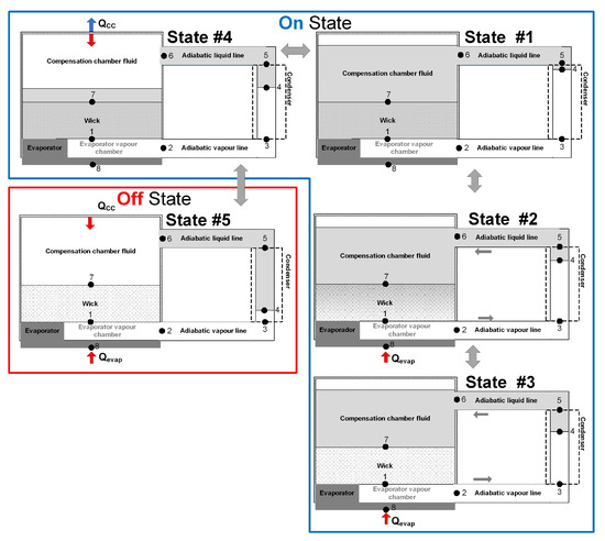
Figure 4.
Operating States of the loop heat pipe as a heat switch.
To integrate these five operational States in the loop heat pipe mathematical model, it is necessary to add the correction coefficients, and , as follows:
where and are correction coefficients used in , from Equation (32), and , respectively.
The red and blue arrows shown in Figure 4 indicate the boundary condition inputs for heating (red) and cooling (blue).
3. Materials and Methods
3.1. Geometry and Working Fluid
The numerical model presented here is representative of a radial loop heat pipe with similar parameters as in [33], shown in the Table 1:

Table 1.
Loop Heat Pipe input properties for a numerical model.
The objective of the presented results is to show a loop heat pipe working as a heat switch; therefore, no dedicated correlation process was performed in relation to an already validated model [33].
3.2. Numerical Implementation
The system of equations obtained from the lumped parameter model is in the form of
where
This is a system of first-order linear differential equations. Once the initial conditions and boundary conditions are defined correctly, the system can be solved with the help of numerical schemes like Odesolve, returning a solution to an ordinary differential equation (ODE), subject to initial value or boundary value constraint. This numerical model is developed with the use of Mathcad® software 15.0 using ODE solve blocks.
4. Simulation Results
4.1. Loop Heat Pipe Model Validation
In accordance with the geometrical properties provided in Section 3.1, a validated loop heat pipe model [33] was chosen as a reference for this article. To ensure the accuracy and credibility of the presented model, a validation study was conducted by comparing our analytical model with experimental tests performed on a loop heat pipe [33]. Through this rigorous process, we obtained comparable results, thereby validating the lumped parameter model. In Figure 5, the result is visible in the experimental test from [33], and the current model is also visible, where W is applied for 1.4 h on the evaporator (), and the external boundary temperature condition is °C.
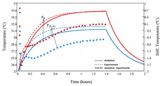
Figure 5.
and response comparisons between modeling results and experimental data. (, C).
The comparison of results in Figure 5 shows a good approximation between the proposed analytical model and experimental tests [33], where the temperature difference at steady-state conditions is approximately C and C, respectively, at and . After 1.4 h, the power is turned off, i.e., W, and the loop heat pipe model returns to the initial temperature state of C.
4.2. Loop Heat Pipe as a Heat Switch
In this section, we show transient simulation results of the developed lumped parameter model, which clarify the operation of the loop heat pipe functioning as a heat switch. Figure 6, Figure 7 and Figure 8 provide valuable insights into the behaviour of a loop heat pipe as a heat switch, clarifying its internal temperature, mass balance, and pressure dynamics.
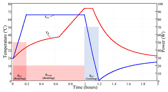
Figure 6.
Chart with changing in temperatures in evaporator and compensation chamber ( and ), and heating/cooling loads ( and ) over time.
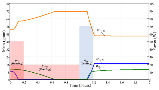
Figure 7.
Chart with changing in liquid masses in condenser, compensation chamber and wick (, and ), and heating/cooling loads ( and ) over time.
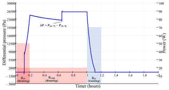
Figure 8.
Chart with changing in differential pressure () and heating/cooling loads ( and ) over time.
The numerical simulation begins from an initial stationary state at an ambient temperature of C, without any heating or cooling power applied. After a few seconds, the evaporator (Node 8) and the condenser (Nodes 3–5) are subjected to a heat power input of W and W, respectively, with a duration of 60 and 12 min as shown in Figure 6. This initiates the temperature increase in the evaporator () and the compensation chamber (), resulting in the natural evaporation of liquid from the Wick (). The liquid inside the compensation chamber () also shows a reduction, as in Figure 7. During this initial period, the pressure differential between the compensation chamber () and the condenser (), denoted as , shows a positive value. This means that there is no liquid flowing from the condenser () to the compensation chamber (), which results in a dry-out of the liquid in , as shown in Figure 7. This dry-out phenomenon first occurs in the compensation chamber () at approximately 0.1 h, followed by the Wick () at approximately 0.65 h.
Once the Wick and the compensation chamber have undergone dry-out, i.e., , the loop heat pipe is considered in an off-state, and its temperature increases linearly, as illustrated in Figure 6, from 0.65 h to 1 h. In this model, there are no significant heat leaks that could cause the temperature of the evaporator (Node 8) and the compensation chamber to cool down and restart the loop heat pipe operation. This means that it forces the device to a start-up.
To demonstrate the functionality of the loop heat pipe as a heat switch device, a cooling effect of W is imposed on the compensation chamber with a duration of 12 min. This restarts the device in an operational mode. In order to initiate the operation, it is crucial to establish a negative pressure differential between the compensation chamber () and the condenser (), i.e., Pa. This pressure differential is essential for facilitating the suction of liquid into compensation chamber and Wick , as illustrated in Figure 8 at 1.1 h.
During the 12 min of W, the compensation chamber temperature reduces linearly to C. At 1.1 h, the liquid inside Wick () and compensation chamber () starts to increase and evaporator temperature starts to decrease.
Finally, without any input heat load, the loop heat pipe returns to the equilibrium ambient temperature of C.
5. Discussion
Loop heat pipes are commonly analysed using various analytical models, including steady-state and transient models. In this study, we presented the lumped parameter model which exhibits thermal performance comparable to that reported by other researchers [33], indicating its reliability. It is worth noting that different authors may adopt distinct modelling approaches, highlighting specific elements of the loop heat pipe or incorporating additional components like radiators in the condenser line with sub-cooling effects, as discussed in [24].
The primary objective of this article was to simulate the heat switch effect that occurs during loop heat pipe dry-out. To achieve this, the model required adjustment parameters. For instance, we set to a value of 50 (W/(m°C)), resulting in a thermal conductance of = 0.267 (W/°C), ensuring reliable behaviour of the condenser. However, it is crucial to correlate this value with dedicated experimental data to enhance the model accuracy in order to find the correct thermal conductance coefficient due to convective effects.
Additionally, the investigation of the convection coefficient between the vapour and condenser lines () is another important aspect that required adjustments to achieve a closer fit between the test data curve from [33] and our model.
During the development of this lumped parameter model, another interesting finding emerged, which highlighted the criticality of correction coefficients, namely and , to simulate the five operational states of the loop heat pipe. Similar to , as suggested in [22,23], these correction factors account for the influence of Wick dry-out.
Interpreting these results in light of previous studies and working hypotheses, it is evident that the lumped parameter model demonstrates thermal performance consistent with that in the established literature, validating its efficacy as a modelling approach for studying the heat switch effect during loop heat pipe dry-out. However, further investigation is warranted to refine and validate the model by comparing it with experimental data and exploring the convection coefficient between the vapour and condenser lines () in greater detail.
An intriguing discovery emerged during the analysis of simulated results, as illustrated in Figure 6, Figure 7 and Figure 8. This discovery relates to the connection between the startup event, occurring at h, and the cooling process () within the time frame of 1 to h, specifically at the compensation chamber. In these figures (Figure 6, Figure 7 and Figure 8), a significant observation is that initiates cooling before the compensation chamber completes its cooling phase, which concludes at 1.2 h. This phenomenon can be attributed to the negative pressure differential () between the compensation chamber () and the condenser (), defined as , as observed in Figure 8. This pressure differential plays a crucial role in facilitating the inflow of liquid into the compensation chamber () and the Wick (), as depicted in Figure 8 at 1.1 h, enabling the device to restart. This means that the start-up of the device could be achieved even with reduction in cooling power () or its time frame. Given the transient nature of heat switch thermal simulations, a transient model proves to be a valuable tool, facilitating dimensioning and allowing for the determination of the appropriate amount of heating or cooling power and the respective application period.
From a broader perspective, this research contributes to the existing knowledge on loop heat pipes by offering insights into their behaviour during dry-out and also highlighting the significance of accurate parameter adjustment and correlation with experimental data. Future research endeavours should concentrate on refining the model by incorporating additional components such as condenser plates and examining other aspects of loop heat pipe operation, such as the impact of dry-out effects and the optimization of thermal conductance values like and .
6. Conclusions
In this study, we developed a lumped parameter model that incorporates solid and fluidic networks to analyse the behaviour of a wicked heat pipe. By formulating a system of first-order linear differential equations, we obtained a comprehensive mathematical representation of the loop heat pipe operation. The model was solved using Mathcad ODEsolver and validated through comparisons with experimental data from the literature. Notably, we successfully demonstrated the loop heat pipe’s effectiveness as a heat switch device. Our investigation led to several key conclusions.
Firstly, we found that the lumped parameter model exhibits excellent agreement with experimental results, underscoring its potential as a tool for evaluating the performance of loop heat pipes as heat switch devices. The model’s ability to replicate experimental outcomes validates its reliability and accuracy.
Secondly, our study introduced a novel mathematical model capable of predicting the transient behaviour of loop heat pipes as a heat switch. By adopting an innovative approach to switch the loop heat pipe on and off, we unlocked the possibility of leveraging loop heat pipes as heat switch devices. This advancement expands the application potential of loop heat pipe technology.
Furthermore, we identified the convective heat transfer coefficient, denoted by h, as a critical factor influencing the performance of loop heat pipes as heat switch devices. This coefficient plays a crucial role in facilitating heat transfer between the compensation chamber canister and its fluid, as well as between the vapour and the condenser pipe. To ensure accurate predictions, it is imperative to correlate the h coefficient using experimental data, enhancing the model’s reliability.
To simulate the five operational states of the loop heat pipe effectively, we introduced a set of corrective coefficients, namely and . These coefficients were essential for accurately capturing the intricate dynamics of the loop heat pipe system, enabling us to analyze and understand its behaviour comprehensively.
Moreover, we observed that applying cooling power to the compensation chamber resulted in a reduction in pressure within the chamber, leading to the cooling of the evaporator. This cooling effect played a crucial role in restarting the fluid loop within the loop heat pipe. Our current model provides valuable insights into estimating the required cooling power for successful loop heat pipe startup, aiding in the design and optimization of loop heat pipe-based systems.
While our research made significant strides, further improvements to the mathematical model are necessary to broaden its applicability. Specifically, simulating loop heat pipes with different geometries and achieving higher accuracy requires a more detailed representation of the processes occurring within the compensation chamber. By refining the model and incorporating these enhancements, we can advance our understanding of loop heat pipes and unlock their full potential in various engineering applications.
The conclusion of this article highlights the suitability of a lumped parameter model as a mathematical approach for predicting the non-linear behaviour of a loop heat pipe operating as a heat switch. However, in order to determine the fidelity and limitation of this non-linear behaviour, it is advisable to perform a model correlation against dedicated test campaigns.
As a future development on the validation of these devices, a valuable recommendation is to establish a correlation between this simplified model and more advanced simulation software such as Thermal Desktop® 6.3 and ESATAN® 2023 that use specialised toolboxes for loop heat pipes.
Author Contributions
Conceptualisation, J.P.C., R.M. and P.G.; methodology, J.P.C., R.M. and P.G.; software, J.P.C.; validation, N.G.D., R.M., P.G. and A.R.R.S.; investigation, J.P.C.; resources, R.M.; data curation, J.P.C.; writing—original draft preparation, J.P.C.; writing—review and editing, N.G.D., R.M., P.G., A.R.R.S. and R.M.P.; visualisation, J.P.C.; supervision, R.M., P.G. and A.R.R.S.; project administration, R.M. and P.G.; funding acquisition, R.M. All authors have read and agreed to the published version of the manuscript.
Funding
The authors acknowledge the support provided by the Research project called Mobilising Agenda: New Space Portugal (Ref. C644936537-00000046, Notice ACC02/CO5-i01/2022, funded by the “Mobilising Agendas for Business Innovation” through the “Recovery and Resilience Programme (PRR)” and by Portugal 2020 through the Competitiveness and Internationalisation Operational Programme and the Lisbon Regional Operational Programme and co-financed by “FEDER”; by FCT, through: CENTRA, project UIDB/00099/2020; IDMEC, under LAETA (Laboratório Associado em Energia, Transportes e Aeronáutica), Project UIDB/50022/2020; AEROG under LAETA, Project UIDB/50022/2020; Project UIDP/50022/2020, Project LA/P/0079/2020.
Institutional Review Board Statement
Not applicable.
Informed Consent Statement
Not applicable.
Data Availability Statement
Data are contained within the article.
Conflicts of Interest
The authors declare no conflict of interest.
Abbreviations
The following abbreviations are used in this manuscript:
| HS | heat switch |
| GGHS | gas-gap heat switch |
| LHP | loop heat pipe |
| Evap | evaporator |
| CC | compensation chamber |
| LPM | lumped parameter model |
| ODE | ordinary differential equations |
| input heat power on the evaporator, W | |
| input heat/cool power on the evaporator, W | |
| T | temperature of node(s), °C |
| M | mass of node(s), kg |
| specific heat at constant pressure, J/(kg·°C) | |
| thermal capacitance of node(s), J/°C | |
| G | thermal conductance, W/°C |
| fluid storage capacitance, s·m | |
| P | absolute pressure, Pa |
| volumetric flow rate, m/s | |
| volumetric mass density of vapour, kg/m | |
| t | time, s |
| volume of stored vapour, m | |
| adiabatic index | |
| specific gas constant, J/(kg·K) | |
| universal gas constant, J/(K·mol) | |
| vapour temperature, K | |
| fluid inductance, 1/m | |
| fluid tube effective length, m | |
| vapour hydraulic area, m | |
| convective surface area, W/(mC) | |
| fluid flow resistance, sm | |
| thermal resistance, °C/W | |
| L | length, m |
| k | thermal conductivity, W/(m·°C) |
| outside diameter, m | |
| internal diameter, m | |
| h | convective heat transfer, W/(mC) |
| equivalent thermal conductivity of Wick, W/(m·°C) | |
| thermal conductivity of solid, W/(m·°C) | |
| thermal conductivity of liquid, W/(m·°C) | |
| Wick porosity, % | |
| V | volume, m |
| fluid latent heat, J/kg | |
| input heat power, W | |
| mass flow rate, kg/s | |
| fluid atomic weight, g/mol | |
| Clausius–Clapeyron relation at saturation curve, g/mol | |
| fluid dynamic viscosity, Pa·s | |
| Wick permeability, m | |
| capillary pressure generated between liquid/vapour, Pa | |
| capillary meniscus radius, Pa | |
| fluid surface tension, N/m | |
| correction coefficient to account the Wick dry-out | |
| correction coefficient on | |
| correction coefficient on |
References
- Shukla, K. Heat Pipe for Aerospace Applications—An Overview. J. Electron. Cool. Therm. Control. 2015, 5, 1–14. [Google Scholar] [CrossRef]
- Bao, K.; Zhuang, Y.; Gao, X.; Xu, Y.; Wu, X.; Han, X. Transient Numerical Model on the Design Optimization of the Adiabatic Section Length for the Pulsating Heat Pipe. Appl. Sci. 2021, 11, 9432. [Google Scholar] [CrossRef]
- Maidanik, Y.; Fershtater, Y.; Solodovnik, N. Loop Heat Pipes: Design, Investigation, Prospects of Use in Aerospace Technics. In Proceedings of the Name of the Aerospace Atlantic Conference and Exposition, Dayton, OH, USA, 18–22 April 1994; pp. 1–9. [Google Scholar]
- Su, Q.; Chang, S.; Zhao, Y.; Zheng, H.; Dang, C. A review of loop heat pipes for aircraft anti-icing applications. Appl. Therm. Eng. 2018, 130, 528–540. [Google Scholar] [CrossRef]
- Shu, Q.S.; Demko, J.A.; Fesmire, J.E. Heat switch technology for cryogenic thermal management. Iop Conf. Ser. Mater. Sci. Eng. 2017, 278, 012133. [Google Scholar] [CrossRef]
- Morgante, G.; Pearson, D.; Melot, F.; Stassi, P.; Terenzi, L.; Wilson, P.; Hernandez, B.; Wade, L.; Gregorio, A.; Bersanelli, M.; et al. Cryogenic characterization of the Planck sorption cooler system flight model. J. Instrum. 2009, 4, T12016. [Google Scholar] [CrossRef]
- Development of a Sorption-Based JT Cooler for the METIS Instrument on E-ELT. Available online: https://indico.cern.ch/event/344330/contributions/806904/attachments/677968/931467/CEC_2015_Ter_Brake_JT_cooler_for_METIS.pdf (accessed on 13 July 2023).
- Barreto, J.; Martins, D.; Branco, M.C.; Branco, J.; Gonçalves, A.P.; Tirolien, T.; Bonfait, G. Hydrogen gas gap heat switch operating in the 150 K to 400 K temperature range. Cryogenics 2021, 119, 103365. [Google Scholar] [CrossRef]
- Barreto, J.; Martins, D.; Branco, M.B.C.; Branco, J.; Ribeiro, R.P.P.L.; Esteves, I.A.A.C.; Mota, J.P.B.; Gonçalves, A.P.; Tirolien, T.; Bonfait, G. 80 K vibration-free cooler for potential future Earth observation missions. IOP Conf. Ser. Mater. Sci. Eng. 2020, 755, 012016. [Google Scholar] [CrossRef]
- Barreto, J. Development of a 40 K to 80 K Vibration-Free Cooler for Future Earth Observation Missions. Ph.D. Thesis, Faculdade de Ciências e Tecnologia, Universidade Nova de Lisboa, Lisboa, Portugal, October 2020. [Google Scholar]
- Catarino, I.; Bonfait, G.; Duband, L. Neon gas-gap heat switch. Cryogenics 2008, 48, 17–25. [Google Scholar] [CrossRef]
- Vanapalli, S.; Keijzer, R.; Buitelaar, P.; ter Brake, H.J.M. Cryogenic flat-panel gas-gap heat switch. Cryogenics 2016, 78, 83–88. [Google Scholar] [CrossRef]
- Vanapalli, S.; Colijn, B.; Vermeer, C.; Holland, H.; Tirolien, T.; ter Brake, H.J.M. A Passive, Adaptive and Autonomous Gas Gap heat Switch. Phys. Procedia 2015, 67, 1206–1211. [Google Scholar] [CrossRef][Green Version]
- Shinozaki, K.; Nohara, T.; Ando, M.; Okamoto, A.; Maeda, M.; Sugita, H.; Takada, S. Research and Development of Heat Switch for Future Space Missions. Trans. Jpn. Soc. Aeronaut. Space Sci. 2014, 12, 7–11. [Google Scholar] [CrossRef]
- Franco, J.; Galinhas, B.; Sousa, P.B.; Martins, D.; Catarino, I.; Bonfait, G. Building a Thinner Gap in a Gas-Gap Heat Switch. Phys. Procedia 2015, 67, 1117–1122. [Google Scholar] [CrossRef]
- Prina, M.; Bhandari, P.; Bowman, R.C., Jr.; Paine, C.G.; Wade, L.A. Development of Gas Gap Heat Switch Actuator for the Planck Sorption Cryocooler. Adv. Cryog. Eng. 2000, 45, 553–560. [Google Scholar]
- Bowman, R.C., Jr. Metal Hydride Compressors with Gas-Gap Heat Switches: Concept, Development, Testing, and Space Flight Operation for the Planck Sorption Cryocoolers. Inorganics 2019, 7, 139. [Google Scholar] [CrossRef]
- Dermenakis, S. Thermal Characterization of a Gas-gap Heat Switch for Satellite Thermal Control. Master’s Thesis, Faculty of Aerospace Engineering, Delft University of Technology, Delft, The Netherlands, January 2016. [Google Scholar]
- Martins, D.F. Desenvolvimento, Construção e Teste de um Interruptor Térmico Para Baixas Temperaturas. Master’s Thesis, Faculdade de Ciências e Tecnologia, Universidade Nova de Lisboa, Lisboa, Portugal, 2010. [Google Scholar]
- Mishkinis, D.; Corrochano, J.; Torres, A. Development of Miniature Heat Switch Temperature Controller based on variable conductance LHP. In Proceedings of the Second International Conference “Heat Pipes for Space Application” (2HPSA), Moscow, Russia, 15–19 September 2014; pp. 1–9. [Google Scholar]
- Ku, J. Methods of Controlling the Loop Heat Pipe Operating Temperature. In Proceedings of the 38th International Conference on Environmental Systems, San Francisco, CA, USA, 29 June–2 July 2008; pp. 1–13. [Google Scholar]
- Ferrandi, C.; Iorizzo, F.; Mameli, M.; Zinna, S.; Marengo, M. Lumped parameter model of sintered heat pipe: Transient numerical analysis and validation. Appl. Therm. Eng. 2013, 50, 1280–1290. [Google Scholar] [CrossRef]
- Kolliyil, J.J.; Yarramsetty, N.; Balaji, C. Numerical Modeling of a Wicked Heat Pipe Using Lumped Parameter Network Incorporating the Marangoni Effect. Heat Transf. Eng. 2020, 42, 787–801. [Google Scholar] [CrossRef]
- Vlassov, V.J.; Riehl, R.R. Mathematical model of a loop heat pipe with cylindrical evaporator and integrated reservoir. Appl. Therm. Eng. 2007, 28, 942–954. [Google Scholar] [CrossRef]
- Koulocheris, D.; Vossou, C. Sensitivity Analysis of a Driver’s Lumped Parameter Model in the Evaluation of Ride Comfort. Vehicles 2023, 5, 1030–1045. [Google Scholar] [CrossRef]
- Florez, F.; Alzate-Grisales, J.A.; Fernández de Córdoba, P.; Taborda-Giraldo, J.A. Methodology for Modeling Multiple Non-Homogeneous Thermal Zones Using Lumped Parameters Technique and Graph Theory. Energies 2023, 16, 2693. [Google Scholar] [CrossRef]
- Ding, X.; He, Y.; Chen, Y.; Wang, Y.; Long, L. Integrated Thermofluid Lumped Parameter Model for Analyzing Hemodynamics in Human Fatigue State. Bioengineering 2023, 10, 368. [Google Scholar] [CrossRef]
- Fernández de Córdoba, P.; Montes, F.F.; Martínez, M.E.I.; Carmenate, J.G.; Selvas, R.; Taborda, J. Design of an Algorithm for Modeling Multiple Thermal Zones Using a Lumped-Parameter Model. Energies 2023, 16, 2247. [Google Scholar] [CrossRef]
- Deng, S.; Li, F.; Luo, H.; Yang, T.; Ye, F.; Chahine, R.; Xiao, J. Lumped Parameter Modeling of SAE J2601 Hydrogen Fueling Tests. Sustainability 2023, 15, 1448. [Google Scholar] [CrossRef]
- Bozkurt, S.; Bozkurt, S. Computational Modelling of Cerebral Blood Flow Rate at Different Stages of Moyamoya Disease in Adults and Children. Bioengineering 2023, 10, 77. [Google Scholar] [CrossRef] [PubMed]
- Mo, S.; Hu, P.; Cao, J.; Chen, Z.; Fan, H.; Yu, F. Effective Thermal Conductivity of Moist Porous Sintered Nickel Material. Int. J. Thermophys. 2006, 27, 304–313. [Google Scholar] [CrossRef]
- Asselman, G.A.A.; Green, D.B. Heat Pipes. Philips Tech. Mag. 1973, 33, 104–113. [Google Scholar]
- Bai, L.; Lin, G.; Wen, D. Modeling and analysis of startup of a loop heat pipe. Appl. Therm. Eng. 2010, 30, 2778–2787. [Google Scholar] [CrossRef]
Disclaimer/Publisher’s Note: The statements, opinions and data contained in all publications are solely those of the individual author(s) and contributor(s) and not of MDPI and/or the editor(s). MDPI and/or the editor(s) disclaim responsibility for any injury to people or property resulting from any ideas, methods, instructions or products referred to in the content. |
© 2023 by the authors. Licensee MDPI, Basel, Switzerland. This article is an open access article distributed under the terms and conditions of the Creative Commons Attribution (CC BY) license (https://creativecommons.org/licenses/by/4.0/).