Abstract
The loading rate of tectonic stress is not constant during long-term geotectonic activity and significantly affects the earthquake nucleation and fault rupture process. However, the mechanism underlying the loading rate effect is still unclear. In this study, we conducted a series of experiments to explore the effect of the loading rate on earthquake nucleation and stick–slip characteristics. Through lab experiments, faults were biaxially loaded at varying rates to produce a series of earthquakes (stick–slip events). Both shear strain and fault displacement were monitored during these events. The findings indicate a substantial effect of the loading rate on the recurrence interval and the shear stress drop of these stick–slip events, with the recurrence interval inversely proportional to the loading rate. The peak friction of the fault also decreases with the increasing loading rate. Notably, prior to the dynamic rupture of earthquakes, there exists a stable nucleation phase where slip occurs in a quasi-static manner. The critical nucleation length, or the distance required before the dynamic rupture, diminishes with both the loading rate and normal stress. A theoretical model is introduced to rationalize these observations. However, the rupture velocity of these lab-simulated earthquakes showed no significant correlation with the loading rate. Overall, this study enhanced our comprehension of earthquake nucleation and rupture dynamics in diverse tectonic settings.
1. Introduction
It has been widely accepted that stick–slip is the mechanism of shallow earthquakes [1]. A stick–slip cycle is usually divided into two stages (i.e., stick and slip). In the stick stage, the shear stress accumulates along the fault with the gradually increasing loading. Once the stress reaches the yield point, the fault will rupture dynamically, leading to a sudden release of the shear stress and rapid frictional sliding of the fault. This stage is called the slip stage. The study of stick–slip is crucial for understanding earthquake mechanisms and fault dynamics. Recent observations of stick–slip events in laboratory faults enabled us to obtain detailed knowledge of stick–slip behaviors and the rupture process of faults [2,3,4,5].
One of the most intriguing findings about stick–slip events confirmed by laboratory studies is that there is a stable nucleation phase preceding unstable dynamic ruptures. In this phase, the rupture zone expands slowly, and aseismic fault slip accumulates in this zone [5,6,7]. In a word, the earthquake nucleation phase represents the initial processes and interactions leading to the final earthquakes [5]. Generally, the earthquake nucleation phase is divided into two stages: (1) the quasi-static growth of rupture from the nucleus, (2) and the acceleration of rupture expansion until reaching the critical nucleation length. Reports exist of indirect observations concerning processes potentially associated with the nucleation phase of certain earthquakes [8,9,10]. Recently, the accelerated slip phase accompanied by a swarm of earthquakes was recognized weeks to months before major earthquakes [11,12]. Particularly, two slow slip transients propagating toward the epicenter of the 2011 Mw 9.0 Tohoku-Oki earthquake were believed to promote the occurrence of the mainshock [9]. Since the occurrence time and location of mainshocks are intimately related to the nucleation process [13], understanding the mechanism of earthquake nucleation is of great importance for earthquake prediction.
Over the past few decades, many efforts have been devoted to quantitatively characterizing the earthquake nucleation process, especially the factors controlling the critical nucleation length. Laboratory experiments [14,15,16,17] and numerical simulations [18] showed that the critical nucleation length scales inversely with the normal stress, which is consistent with the prediction from the theoretical model [19]. Another factor that may control the rupture behaviors of faults is the loading rate [20,21,22,23,24]. The loading rate of natural faults, typically determined through geodetic measurements, can be significantly influenced by the creep of adjacent segments along the fault system. This phenomenon can result in local loading rates that vary by order of magnitude compared to the overall tectonic loading rate, causing substantial differences in stress accumulation along the fault [25,26,27,28]. Some laboratory experiments and theoretical investigations showed that a higher loading rate contributes to a transition from stick–slip to stable slip [20,22,29,30,31]. On the contrary, some experimental results suggested that a higher loading rate may promote unstable slip [3,6,32] or favor ruptures with higher speed [33]. It was also suggested that the impact of loading rates on fault slip behaviors hinges on the fault’s proximity to a steady state. While typically higher rates drive faults away from steadiness, causing increased instability, in the context of stiff loading systems applying constant, high rates, faults are instead nudged toward a steady state, resulting in stable sliding [15]. This nuanced interaction underscores the complexity of fault responses in varying loading scenarios and surroundings [34].
Furthermore, the loading rate could also affect the nucleation process of earthquakes. An early laboratory experiment confirmed that the critical nucleation length decreases with the increase in the loading rate [6]. Specifically, the nucleation length decreases exponentially with the increase in the loading rate [35]. In addition, the spatial distribution of the nucleation zone is also influenced by the loading rate. At a high loading rate, the nucleation is concentrated in some specific locations, while the nucleation location is randomly scattered at a lower loading rate [35]. On the contrary, it was suggested that the initial rupture location tends to concentrate on the same patch at a low loading rate but is randomly distributed at a high loading rate [33]. Despite abundant field observations and laboratory investigations, the effect of the strain rate or the loading rate on the earthquake nucleation and rupture dynamics remains enigmatic.
In this study, we conducted highly constrained earthquake experiments, focusing on the influence of the loading rate on the earthquake nucleation and rupture dynamics. Through precise strain monitoring and high-speed photography, we monitored the spatial–temporal evolution of displacement fields. Our detailed analysis led to the development of an empirical model that integrates the effects of both the loading rate and the stress state, significantly enhancing our understanding of the earthquake nucleation process.
2. Materials and Methods
2.1. Fault Samples Acquisition
The fault sample was made of polymethyl methacrylate (PMMA), a commonly used material in laboratory investigations of earthquakes due to its low wave velocity, homogeneity, and tractability [35,36]. The physical properties of PMMA are shown in Table 1. As shown in Figure 1, the specimen is composed of two triangular PMMA plates. A frictional interface (700 × 20 mm) mimicking the fault was formed when the two plates were held together. The interface surfaces were polished to an overall roughness of less than 1 µm.

Table 1.
Properties of PMMA.
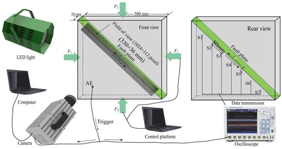
Figure 1.
Schematic diagram of the experimental settings. The experimental setup consists of a biaxial-loading apparatus, a fault model, a high-speed camera, a stress monitoring system, and a LED light. The fault plane is highlighted in green. The rectangular region (field of view) enclosing the fault is textured with speckle patterns, and the images of the field of view are taken by the high-speed camera. Shear strain near the fault is obtained by the strain rosette.
2.2. Experimental Setup
The configuration of the self-developed servo-controlled biaxial system is displayed in Figure 1. Four jacks were controlled independently, and the force was recorded at a sampling rate of 100 Hz, with an accuracy of 0.01 kN. In our experiments, the horizontal stress (σx) and vertical stress (σy) were simultaneously increased to 1 MPa at a rate of 0.01 MPa/s. Then, the stress state was held for 30 min to achieve a stable state. After that, the jacks in the vertical direction were instructed to move at a certain rate to load the fault while σx was held constant. With the successive increase in σy, a sequence of stick–slip events occurred on the fault in each run, at nearly constant recurrence intervals.
Figure 2 illustrates the typical displacement and load–time history curves obtained during the experiments. The curves demonstrate the system stability throughout the stress maintenance phase and the linear stress increasing during the loading phase, facilitated by the servo control system. Notably, a sequence of stick–slip events is evident. Each fault instability episode is marked by synchronous displacement in the y-direction platen (highlighted by the red line) and an abrupt, transient fluctuation in the x-direction load, which is promptly corrected by the biaxial press servo control to maintain the predetermined load. The shear stress (τ) and normal stress (σn) acting on the fault can be derived from the biaxial forces:
where F1 and F2 are the horizontal and vertical forces, respectively. A = 0.01 m2 is the lateral area of the sample. In this study, the fault was loaded at seven sets of rates, i.e., 0.5, 1.0, 1.5, 2.0, 2.5, 3.0, and 3.5 µm/s. To suppress the effect of slip history, we cleansed the fault surface with water after each run.
τ = (F2 − F1)/2A
σn = (F2 + F1)/2A
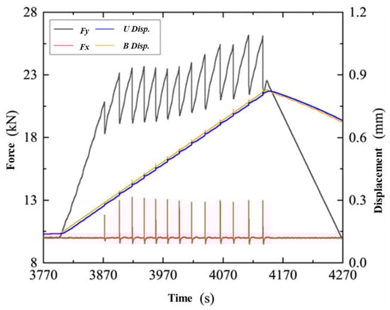
Figure 2.
Typical time history curves for displacement and load during experimental runs. The black line denotes the vertical load, while the red line denotes the horizontal load. Displacements from the upper jack and bottom jack are represented by the blue and orange lines, respectively.
2.3. Diagnostic Method
To probe the nucleation and rupture process of the laboratory earthquakes, we developed a monitoring method to simultaneously monitor the full-field displacement and the shear strain along the fault. Combining these two diagnostic methods facilitates the retrieval of accurate information about laboratory earthquakes.
2.3.1. Full Field Displacement
In this study, a Photron FASTCAM SA1.1 high-speed camera, with a capability to record at 50,000 frames per second (fps), was utilized to monitor the textured fault field of view (Figure 1). It possesses a buffer for 400 frames both before and after the trigger. The resolution at this speed stands at 1024 × 112 pixels, which translates to a physical domain of 330 × 36 mm. To quantitatively deduce the dynamic displacement during an earthquake simulated in the lab, digital image correlation (DIC) was used. Random speckle of monodispersed black dots was imprinted on a PMMA sheet’s surface, positioned orthogonally to the fault’s plane. DIC evaluations were calculated using the VIC-2D software version 6 by Correlation Solutions Inc., Irmo, SC, USA. by leveraging the “Fill Boundary” algorithm. This specific algorithm is adept at deciphering shear offsets at displacement discontinuities. For our calculations, a subset size of 21 × 21 pixels, approximately 10.25 mm, was selected with an incremental step of three pixels (approximately 1.5 mm). No averaging was conducted across multiple subsets, maintaining a consistent DIC parameter set that provided a holistic view of the displacement field for all experiments. Detailed error analysis can be found in a separate study [37].
2.3.2. Shear Strain
Seven groups of strain rosette were pasted along the fault on the back of the sample. These strain rosettes were located 1 mm away from the fault and spaced regularly, about 80 mm apart. The seismic wave was generated and propagated in the sample as stick–slip occurred, and the electrical signals were obtained by the ultrasonic sensor due to the piezoelectric effect when the seismic wave arrived. To avoid losing the small signal and ensure the signals are up to the trigger threshold of the high-speed camera and data acquisition system (DAQ), the electrical signals were amplified by 40 dB by the AE amplifiers. The signal sampling rate was set as 1 MHz, and the total recording duration was 8 ms, with the trigger point in the center of the duration. It should be noted that the electrical signals simultaneously triggered the DAQ and high-speed camera.
2.4. System Stiffness
Previous studies showed that the system’s stiffness significantly influences the stability of fault sliding [38]. A spectrum of fault slip behaviors can be produced by adjusting the stiffness, ranging from stable fault creep and slow slip events to unstable ruptures [38]. Unstable ruptures tend to occur if the system’s stiffness is reduced to a critical value [39]. In addition, a previous study estimated both the loading and unloading stiffness to pick data and to avoid the experimental result bias because of the unintentional variation in the system stiffness [33]. Thus, in this study, to isolate the loading rate effect on the fault slip behaviors, we needed to ensure that the loading and unloading stiffness of the loading system was independent of the loading rate.
2.4.1. Loading Stiffness
In this paper, the loading stiffness is defined as the ratio of vertical stress increment over vertical displacement increment. The vertical force fluctuates in the early stage of the loading stage; we thus selected the 50% data in the middle of the loading stage in the recurrence interval to calculate the loading stiffness of the upcoming stick–slip event (the red portion of Figure 3a,b). After counting the stiffness data of all the events (Figure 3c), we can discover that the loading stiffness at different loading rates is almost the same. We fitted the curve based on the data of the vertical stress increment and the vertical displacement increment as Δσy = 0.0103 ΔD and R2 = 0.99, and estimated that the macroscopic loading stiffness was 10.3 GPa/m. The results showed that the system runs consistently in the loading stage.
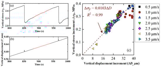
Figure 3.
Temporal evolutions of (a) vertical stress and (b) vertical displacement; the red segments in (a,b) are used to calculate the loading stiffness presented in (c). (c) Vertical stress increment versus vertical displacement increment and the loading stiffness fitted by the data. Both stress and displacement are recorded from the loading machine.
2.4.2. Unloading Stiffness
We summarized the relationship between the shear stress drop and fault displacement at different loading rates, as shown in Figure 4. The unloading stiffness of the system is defined as the stress drop corresponding to unit displacement, which is represented as the slope in Figure 4. The line slope corresponds to the macroscopic stiffness of the unloading system of 1.9 GPa/m. This result shows that the macroscopic stiffness of the system has a slight fluctuation under different conditions. Therefore, we can conclude that the system runs stably, and the loading rate has nearly no effect on the system loading and unloading stiffness. The experiment system can be used to research the loading rate effect on the nucleation mechanism and rupture dynamics.
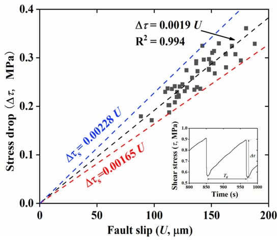
Figure 4.
Macroscopic shear stress drop–displacement curve at different loading rates. The black squares represent the shear stress drop at each fault slip. The blue and red lines represent the upper and lower limits of the stiffness fluctuation of the system, respectively. The inset shows the definition of shear stress drop and the fault slip defined as the fault displacement during a slip event. The fault slip is derived from DIC measurements.
3. Results
In this section, we first present the general mechanical results of the stick–slip events. Then, the results of the loading rate effects on the earthquake nucleation and rupture dynamics are presented.
3.1. Stick–Slip Events
Figure 5 shows the vertical stress (σy) as a function of time for seven sets of experiments with different loading rates. Each set of experiments is characterized by repeated stick–slip events, where the stress continuously accumulates during the interseismic “stick” stage and abruptly releases in the coseismic “slip” stage. After the first several runs, the stick–slip cycles gradually become periodic, with the recurrence interval nearly constant. This typical stick–slip behavior has been widely reported in previous experiments with various materials [21,23,33].
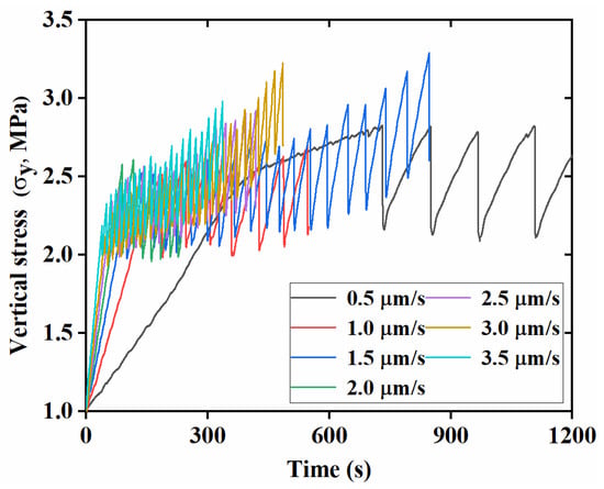
Figure 5.
Vertical stress evolution for faults at different loading rates.
3.2. Effect of Loading Rate on the Features of Stick–Slip Events
3.2.1. Shortening in Recurrence Interval
The recurrence interval is defined as the time interval between the two adjacent stick–slip events, as illustrated in Figure 6a. The effect of the loading rate on the recurrence interval is shown in Figure 6b. The recurrence intervals decrease with the increase in the loading rate. Previous studies [22] showed that there is a power–law relationship between the recurrence interval and the loading rate:
where m is the scaling constant, and n is the power–law exponent. Importantly, n determines the time-dependent effect of frictional strength: n > −1 corresponds to the time-dependent weakening effect; n = −1 indicates that the static stress drop is not affected by the recurrence interval, and there is no time-dependent strengthening; n < −1 means the time-dependent strengthening of the fault strength [40]. For this work, the experimental results in Figure 6b are fitted as follows:
TR = m (VL)n
log TR = nlog VL + m
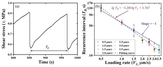
Figure 6.
(a) Shear stress versus time for the case with a loading rate of 0.5 µm/s, where TR is the recurrence interval of a stick–slip event. (b) TR as a function of loading rate. The dotted line is the fitted curve based on the data, while the solid line is the reference line with a slope of 1 which is used to distinguish whether the fault is strengthened or not.
The n is fitted as −1.201, indicating a time-dependent strengthening of the fault strength. A recent study [23] found that n is equal to −1.252 through stick–slip experiments on granite blocks simulating a fault, which is similar to our results.
3.2.2. Static Friction
Figure 7a shows the ratio between the shear stress and the normal stress as a function of time in the stick–slip cycles. This ratio increases linearly with the time during the interseismic stage until it reaches its peak values (static friction, μp) and then drops sharply in the coseismic stage. We define the friction drop (∆μ) as the difference between the peak friction μp and the residual friction μmin, i.e., ∆μ = μp − μmin. Figure 7b describes the peak friction coefficient μp as a function of loading rate. Generally, the peak friction decreases with the increase in the loading rate, despite the scattering. An exponential function is used to fit the results:
µp = 0.048 VL−0.455 + 0.414
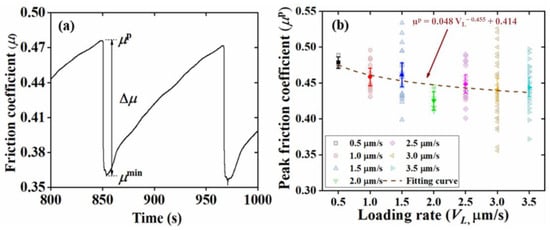
Figure 7.
(a) Friction coefficient–time curve defining the static friction (μp), the minimum friction (μmin), and the friction drop (∆μ). (b) Static friction (μp) as a function of loading rate. The light color symbols represent the actual value. The highlight color symbols are the mean values with a 95% confidence interval. The dotted line is the fitting curve based on the mean values at different loading rates.
Figure 8 shows the static friction as a function of recurrence interval. The static friction increases with the logarithm of the recurrence interval, which is consistent with previous results [41,42]. This positive correlation between the static friction and the recurrence interval is also consistent with the time-dependent strengthening of the fault strength suggested by Equation (5). It has been proved that the time-dependent strengthening of the fault strength may arise from the increase in the real area of adhesive contacts with time, which may be due to the localized creep and the degradation of contact hardness [43]. Thus, a lower loading rate may allow for more development of the time-dependent inelastic behaviors of the contacts, leading to larger contact areas.
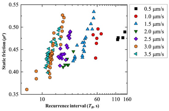
Figure 8.
Static friction versus recurrence interval. At a fixed loading rate, static friction rises logarithmically with recurrence intervals, consistent with the previous findings [41,42].
3.2.3. Stress Drop
The shear stress drop is closely related to the energy release of earthquakes and is one of the most important parameters of source process. Figure 9a describes the shear stress drop as a function of loading rate. With the increase in the loading rate, the shear stress drop decreases, and the relationship between the shear stress drop and the loading stress is fitted as Δτ = 0.294 VL−0.291. This trend is generally consistent with previous studies [20]. Figure 9b describes the friction drop ∆μ as a function of loading rate, and the curve can be expressed as Δµ = 0.101 VL−0.281 by fitting the data. For friction coefficient drop, it is observed that a lower loading rate guarantees a higher friction coefficient drop by analyzing both the macroscopic and local data [33], which is consistent with our result.
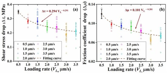
Figure 9.
(a) Stress drop and (b) friction drop as functions of loading rate. The light color symbols represent the actual values. The highlight color symbols are the mean values with a 95% confidence interval. The dotted line is the fitting curve based on the mean values at different loading rates.
3.3. Effect of Loading Rate on Earthquake Nucleation Process
3.3.1. Basic Characteristics of Earthquake Nucleation
The high-speed photography and strain rosette are used to simultaneously monitor the full-field displacement field and the shear stress at multiple locations along the fault at different loading rates. Figure 10 collectively presents the spatiotemporal evolution of the fault slip and the history of the shear stress along the fault from the quasi-static nucleation to the dynamic coseismic rupture. Figure 11 shows the detailed spatiotemporal progression of the rupture fronts at a 0.5 µm/s loading rate. The red line represents a linear fit of the rupture points, with its slope indicating the inverse of the rupture propagation speed. It highlights the contrast between the fast dynamic propagation at 1908 m/s and the notably slower quasi-static progression within the critical length (LC), moving at an approximate 11 m/s—well under the S-wave velocity. In this stage, the shear stress in the nucleation zone is partially released, which may be due to the development of localized pre-slip [4,7]. Dynamic rupture occurs when the size nucleation zone attains a critical length (LC). In the dynamic rupture stage, ruptures always propagate bilaterally at a velocity approaching or even exceeding the S-wave velocity. The abrupt increase in the fault slip corresponds to the abrupt drop in the shear stress, indicating that both the displacement and the shear stress monitoring can disclose the transient rupture process. Previous studies clearly showed that the rupture process can be divided into three stages: quasi-static growth, acceleration, and dynamic rupture [7,14]. Our observations are generally consistent with previous studies.
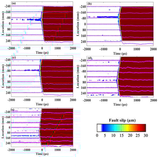
Figure 10.
Evolution process of displacement field and strain during fault nucleation and rupture at loading rates of (a) 0.5 µm/s, (b) 1.0 µm/s, (c) 1.5 µm/s, (d) 2.0 µm/s, and (e) 2.5 µm/s. The nephogram is the location–time view of fault slip evolution; the purple curve represents the shear strain at the corresponding position. Time 0 means the trigger time of displacement and strain monitoring system.
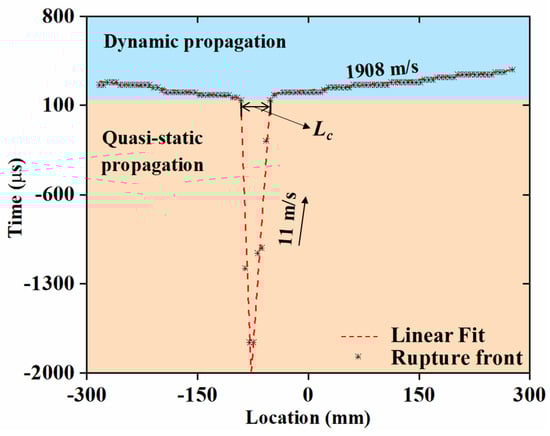
Figure 11.
Diagram illustrating the spatiotemporal distribution of rupture fronts, denoted by asterisk markers, at a loading rate of 0.5 µm/s. The red line provides a linear fit of these rupture points, with its slope signifying the reciprocal of the rupture propagation velocity. The chart distinguishes between the dynamic propagation at 1908 m/s and the more gradual quasi-static propagation with an approximate velocity of 11 m/s, notably below the S-wave velocity.
In addition, we found that the nucleation phase is controlled by the loading rate. As the loading rate increases, the nucleation size gradually decreases. When the loading rate reaches 3.0 µm/s, the nucleation region cannot be observed in the observation system mentioned in this paper. The direct shear experiment based on meter-scale rocks found that the nucleation phase exists at slow (0.01 mm/s) and intermediate (0.1 mm/s) loading rates, while it disappears at a fast loading rate (1 mm/s) [33]. In addition, the relationship between the nucleation length and the loading rate through double shear experiments are studied using high-speed photography and strain rosette [35]. It was found that when the loading rate increased from 0.01 MPa/s to 6 MPa/s, the nucleation length was nearly three times shorter. It is considered that the loading rate affects the nucleation length by modifying the dimensionless variable Vθ/dc in the framework of the rate-and-state constitutive friction law. The minimum nucleation length observed in the experiment is 0.8 cm.
3.3.2. Critical Nucleation Length
The critical nucleation length of the laboratory earthquakes can be determined from the rupture front in Figure 11. Theoretically, critical nucleation length is related to the normal stress and frictional parameters [19]. As shown in Figure 12, the critical nucleation length decreases with the increase in the loading rate when the loading rate is lower than 3.0 µm/s, which is qualitatively consistent with Guérin-Marthe’s results [35]. This result suggests that it may be more difficult to identify the nucleation phase of earthquakes on faults with high loading rates than those with slow loading rates.
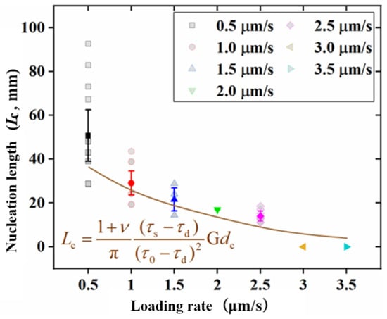
Figure 12.
Nucleation lengths as a function of loading rate. The light color symbols represent the actual values. The dark color symbols are the mean values with a 95% confidence interval. The dotted line is the fitting curve based on the actual values at different loading rates and the theoretical model.
Previous studies explored the underlying mechanism of the loading rate influence on the nucleation size to some extent [33,35]. However, these interpretations were mainly based on qualitative analysis. In this study, we attempted to explain why the nucleation size depends on the loading rate in a quantitative manner. Assuming that the fault friction is governed by the slip-weakening law [44], the critical rupture length can be expressed as follows:
where ν is the Poisson’s ratio, G is the shear modulus, and dc is the critical slip distance; τs = µsσn and τd = µdσn are the static and dynamic friction strengths, respectively; and τ0 = µpσn is the initial friction strength.
Lc = (1 + ν) · (τs − τd) · G · dc/π · (τ0 − τd)2
From Figure 7b, we can see that the loading rate has an effect on the fault strength. It was found that the loading rate influences the sliding mode in a specific range of the normal stress [21]. It was also found that the shear stress drop decreases with the loading rate, and the sliding mode transforms from stick–slip to stable sliding when the loading rate reaches a critical value. This is partly due to the fact that a higher loading rate may prevent the action of adhesion forces on the interlocking asperities. According to the rate and state friction constitutive law, the change in the sliding velocity leads to the change in the coefficient of friction. Thus, we can assume that the loading rate affects the static friction coefficient (µs), and the relationship between µs and the loading rate has the same form as that in the rate-and-state friction constitutive law:
where a and b are the constants. Equation (5) can be transformed as follows:
µs = aln(bVL)
L = Lcσn = (1 + ν) · (µs − µd) · G · dc/π · (µp − µd)2
= (1 + ν) · (aln(bVL) − µd) · G · dc/π · (0.048 VL−0.455 + 0.414 − µd)2
= (1 + ν) · (aln(bVL) − µd) · G · dc/π · (0.048 VL−0.455 + 0.414 − µd)2
Fitting the data in Figure 12 based on Equation (4) yields that a = −0.243, b = 0.156, µd = 0.16, dc = 19.6 µm, µp = 0.048 VL−0.455 + 0.414, and Δµ = 0.101 VL−0.281.
3.3.3. Nucleation Velocity and Duration of Nucleation Phase
Figure 13 shows the effect of the loading rate on the nucleation velocity and duration of the nucleation phase. In this work, the nucleation velocity is defined as the velocity that the nucleation zone expands at. We focus on cases with the loading rate below 3.0 µm/s because it is hard to observe the nucleation phase when the loading rate exceeds 3.0 µm/s. Our results show that the nucleation velocity decreases with the loading rate. Moreover, all the nucleation velocities are below 20 m/s, which is much lower than the S-wave velocity of the sample. The nucleation time varies with loading rate. Overall, a higher loading rate leads to a longer nucleation time. It is thus hard for us to catch the precursor of natural earthquakes because of the much lower loading rate of the tectonic stress.
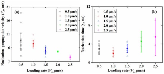
Figure 13.
Nucleation (a) velocity and (b) time as functions of loading rate. The light color symbols represent the actual values. The highlight color symbols are the mean values with a 95% confidence interval.
3.4. Effect of Loading Rate on Rupture Velocity
Figure 14 shows the normalized rupture velocity at different loading rates. VS is the S-wave velocity of the sample. Rupture velocities are calculated from the shear strain recordings. There is no clear relationship between the rupture velocity and the loading rate from Figure 14. Furthermore, the rupture velocity is distributed in the range from about 0.4 VS (sub-Rayleigh wave rupture) to about 1.7 VS (super-shear wave rupture), except the forbidden zone (VR~VS). It is also found that the ruptures are all sub-Rayleigh events [35]. Moreover, one study proposed that the dynamic rupture velocity increases with the loading rate, and that the dynamic rupture velocity can exceed the shear velocity only at the fastest loading rate (1 mm/s in their work) [33]. The above results are different from our results, which may be due to the different loading ways and stress states.
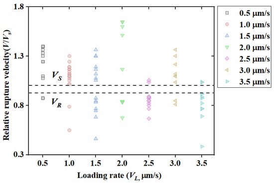
Figure 14.
Summary of relative velocity as a function of loading rate. Two dotted lines refer to the top (VS) and bottom (VR) limitations of the so-called “forbidden zone”.
4. Conclusions
In this work, we studied the characteristics of earthquake nucleation and rupture dynamics at different loading rates. Our findings unveiled several key relationships:
- Recurrence intervals: As the loading rate increases, the recurrence intervals decrease. This suggests that at higher loading rates, faults require less time to accumulate the stress necessary for an earthquake, resulting in more frequent seismic events.
- Frictional dynamics: The peak friction coefficient, the change in the friction coefficient, and the change rate of the friction coefficient decrease with the increasing loading rate. This could imply limited interactions between the fault surfaces at higher rates, potentially undermining the fault’s locking mechanisms.
- Shear stress and energy release: The shear stress drop (or the relative shear stress drop) decreases with the loading rate, which indicates that seismic events at slower loading rates release a more significant portion of accumulated energy. A lower loading rate means a larger recurrence interval and thus longer holding time of the two contact surfaces. This may favor the strengthening of the fault.
- Critical nucleation length: The critical nucleation length decreases with the loading rate. In simpler terms, higher tectonic activities can trigger earthquakes even in shorter fault segments. We propose a theoretical model to explain the loading rate dependence on the critical nucleation length.
- Aseismic slip: Our findings revealed that during the initial stages of the nucleation phase, aseismic or stable slip is the only activity. As the process evolves, this slip shifts towards a cascading process. This observation aligns with the results from other studies [16]. However, a long-lasting question is whether the primary seismic event, or the mainshock, is genuinely initiated by this cascade-like sequence. Essentially, it is debated whether the mainshock is merely an amplified foreshock resulting from the rupture of a sufficiently large or weak segment which then propagates across the entire fault plane. Recent seismic data point to a similarity between small and large earthquakes [45], suggesting that this might indeed be the scenario.
To conclude, we demystified the effects of loading rates on key fault friction parameters, such as the static friction coefficient (µs), the dynamic friction coefficient (µd), and the critical slip distance (dc). These insights are invaluable for a comprehensive understanding of earthquake processes.
Author Contributions
Conceptualization, C.W. and X.L.; methodology, C.W.; software, K.Z.; validation, C.W. and G.W.; formal analysis, G.W.; investigation, G.W.; resources, X.L.; data curation, G.W.; writing—original draft preparation, G.W.; writing—review and editing, C.W.; visualization, K.Z.; supervision, C.W.; project administration, C.W. and X.L.; funding acquisition, X.L. All authors have read and agreed to the published version of the manuscript.
Funding
This research was funded by CNPC Innovation Fund (#2022DQ02-0610).
Institutional Review Board Statement
Not applicable.
Informed Consent Statement
Not applicable.
Data Availability Statement
The data presented in this study are available on request from the corresponding author. The data are not publicly available due to restrictions from the State Key Laboratory.
Acknowledgments
This work was supported by the China Scholarship Council. We also extend our gratitude to Arie Xia of Richmond Hill High School, Ontario, Canada, for his assistance in conducting the experiments and analyzing the data.
Conflicts of Interest
The authors declare no conflict of interest.
References
- Brace, W.F.; Byerlee, J.D. Stick-slip as a mechanism for earthquakes. Science 1966, 153, 990–992. [Google Scholar] [CrossRef] [PubMed]
- Passelègue, F.X.; Schubnel, A.; Nielsen, S.; Bhat, H.S.; Deldicque, D.; Madariaga, R. Dynamic rupture processes inferred from laboratory microearthquakes. J. Geophys. Res. Solid. Earth 2016, 121, 4343–4365. [Google Scholar] [CrossRef]
- McLaskey, G.C.; Yamashita, F. Slow and fast ruptures on a laboratory fault controlled by loading characteristics. J. Geophys. Res. Solid. Earth 2017, 122, 3719–3738. [Google Scholar] [CrossRef]
- McLaskey, G.C.; Kilgore, B.D. Foreshocks during the nucleation of stick-slip instability. J. Geophys. Res. Solid. Earth 2013, 118, 2982–2997. [Google Scholar] [CrossRef]
- Ohnaka, M.; Kuwahara, Y. Characteristic features of local breakdown near a crack-tip in the transition zone from nucleation to unstable rupture during stick-slip shear failure. Tectonophysics 1990, 175, 197–220. [Google Scholar] [CrossRef]
- Kato, N.; Yamamoto, K.; Yamamoto, H.; Hirasawa, T. Strain-rate effect on frictional strength and the slip nucleation process. Tectonophysics 1992, 211, 269–282. [Google Scholar] [CrossRef]
- Ohnaka, M. Earthquake source nucleation: A physical model for short-term precursors. Tectonophysics 1992, 211, 149–178. [Google Scholar] [CrossRef]
- Ellsworth, W.L.; Beroza, G.C. Seismic evidence for an earthquake nucleation phase. Science 1995, 268, 851–855. [Google Scholar] [CrossRef]
- Kato, A.; Obara, K.; Igarashi, T.; Tsuruoka, H.; Nakatani, M.; Hirata, N. Propagation of slow slip leading up to the 2011Mw 9.0 Tohoku-Oki earthquake. Science 2012, 335, 705–708. [Google Scholar] [CrossRef]
- Bouchon, M.; Karabulut, H.; Aktar, M.; Ozalaybey, S.; Schmittbuhl, J.; Bouin, M.P. Extended nucleation of the 1999 Mw 7.6 Izmit earthquake. Science 2011, 331, 877–880. [Google Scholar] [CrossRef]
- Ruiz, S.; Metois, M.; Fuenzalida, A.; Ruiz, J.; Campos, J. Intense foreshocks and a slow slip event preceded the 2014 Iquique Mw 8.1 earthquake. Science 2014, 345, 1165–1169. [Google Scholar] [CrossRef] [PubMed]
- Ruiz, S.; Aden-Antoniow, F.; Baez, J.C.; Otarola, C.; Potin, B. Nucleation phase and dynamic inversion of the Mw 6.9 valparaíso 2017 earthquake in central chile. Geophys. Res. Lett. 2017, 44, 10.290–10.297. [Google Scholar] [CrossRef]
- Dong, P.; Xu, R.; Yang, H.; Guo, Z.; Xia, K. Fault slip behaviors modulated by locally increased fluid pressure: Earthquake nucleation and slow slip events. J. Geophys. Res. Solid. Earth 2022, 127, e2022JB024612. [Google Scholar] [CrossRef]
- Latour, S.; Schubnel, A.; Nielsen, S.; Madariaga, R.; Vinciguerra, S. Characterization of nucleation during laboratory earthquakes. Geophys. Res. Lett. 2013, 40, 5064–5069. [Google Scholar] [CrossRef]
- McLaskey, G.C. Earthquake Initiation from Laboratory Observations and Implications for Foreshocks. J. Geophys. Res. Solid. Earth 2019, 124, 12882–12904. [Google Scholar] [CrossRef]
- Marty, S.; Schubnel, A.; Bhat, H.S.; Aubry, J.; Fukuyama, E.; Latour, S.; Nielsen, S.; Madariaga, R. Nucleation of Laboratory Earthquakes: Quantitative Analysis and Scalings. J. Geophys. Res. Solid. Earth 2023, 128, e2022JB026294. [Google Scholar] [CrossRef]
- Dong, P.; Xia, K. Laboratory investigations probing earthquake source process. Chin. Sci. Bull. 2022, 67, 1378–1389. [Google Scholar] [CrossRef]
- Kaneko, Y.; Nielsen, S.B.; Carpenter, B.M. The onset of laboratory earthquakes explained by nucleating rupture on a rate-and-state fault. J. Geophys. Res. Solid. Earth 2016, 121, 6071–6091. [Google Scholar] [CrossRef]
- Andrews, D.J. Rupture velocity of plane strain shear cracks. J. Geophys. Res. 1976, 81, 5679–5687. [Google Scholar] [CrossRef]
- Teng-Fong, W.; Zhao, Y. Effects of load point velocity on frictional instability behavior. Tectonophysics 1990, 175, 177–195. [Google Scholar] [CrossRef]
- Bouissou, S.; Petit, J.P.; Barquins, M. Normal load, slip rate and roughness influence on the polymethylmethacrylate dynamics of sliding 1. Stable sliding to stick-slip transition. Wear 1998, 214, 156–164. [Google Scholar] [CrossRef]
- Karner, S.L.; Marone, C. Effects of loading rate and normal stress on stress drop and stick-slip recurrence interval. In Geocomplexity and the Physics of Earthquake; Geophysical Monograph Series; American Geophysical Union: Washington, DC, USA, 2000; pp. 187–198. [Google Scholar]
- Zhou, X.; He, Y.; Shou, Y. Experimental investigation of the effects of loading rate, contact roughness, and normal stress on the stick-slip behavior of faults. Tectonophysics 2021, 816, 229027. [Google Scholar] [CrossRef]
- Dong, P.; Xia, K.; Xu, Y.; Elsworth, D.; Ampuero, J.P. Laboratory earthquakes decipher control and stability of rupture speeds. Nat. Commun. 2023, 14, 2427. [Google Scholar] [CrossRef]
- Klein, E.; Bock, Y.; Xu, X.; Sandwell, D.T.; Golriz, D.; Fang, P.; Su, L. Transient deformation in california from two decades of GPS displacements: Implications for a three-dimensional kinematic reference frame. J. Geophys. Res. Solid. Earth 2019, 124, 12189–12223. [Google Scholar] [CrossRef]
- Bacques, G.; de Michele, M.; Raucoules, D.; Aochi, H.; Rolandone, F. Shallow deformation of the San Andreas fault 5 years following the 2004 Parkfield earthquake (Mw6) combining ERS2 and Envisat InSAR. Sci. Rep. 2018, 8, 6032. [Google Scholar] [CrossRef] [PubMed]
- Chaussard, E.; Bürgmann, R.; Fattahi, H.; Johnson, C.W.; Nadeau, R.; Taira, T.; Johanson, I. Interseismic coupling and refined earthquake potential on the Hayward-Calaveras fault zone. J. Geophys. Res. Solid. Earth 2015, 120, 8570–8590. [Google Scholar] [CrossRef]
- De Michele, M.; Raucoules, D.; Rolandone, F.; Briole, P.; Salichon, J.; Lemoine, A.; Aochi, H. Spatiotemporal evolution of surface creep in the Parkfield region of the San Andreas Fault (1993–2004) from synthetic aperture radar. Earth Planet. Sci. Lett. 2011, 308, 141–150. [Google Scholar] [CrossRef]
- Ohnaka, M. Experimental studies of stick-slip and their application to the earthquake source mechanism. J. Phys. Earth 1973, 21, 285–303. [Google Scholar] [CrossRef]
- Logan, J.M.; Teufel, L.W. The effect of normal stress on the real area of contact during frictional sliding in rocks. Pure Appl. Geophys. 1986, 124, 471–485. [Google Scholar] [CrossRef]
- Baumberger, T.; Heslot, F.; Perrin, B. Crossover from creep to inertial motion in friction dynamics. Nature 1994, 367, 544–546. [Google Scholar] [CrossRef]
- Togo, T.; Shimamoto, T.; Yamashita, F.; Fukuyama, E.; Mizoguchi, K.; Urata, Y. Stick–slip behavior of Indian gabbro as studied using a NIED large-scale biaxial friction apparatus. Earthq. Sci. 2015, 28, 97–118. [Google Scholar] [CrossRef]
- Xu, S.; Fukuyama, E.; Yamashita, F.; Mizoguchi, K.; Takizawa, S.; Kawakata, H. Strain rate effect on fault slip and rupture evolution: Insight from meter-scale rock friction experiments. Tectonophysics 2018, 733, 209–231. [Google Scholar] [CrossRef]
- Gounon, A.; Latour, S.; Letort, J.; El Arem, S. Rupture nucleation on a periodically heterogeneous interface. Geophys. Res. Lett. 2022, 49, e2021GL096816. [Google Scholar] [CrossRef]
- Guérin-Marthe, S.; Nielsen, S.; Bird, R.; Giani, S.; Di Toro, G. Earthquake nucleation size: Evidence of loading rate dependence in laboratory faults. J. Geophys. Res. Solid. Earth 2019, 124, 689–708. [Google Scholar] [CrossRef] [PubMed]
- Ben-David, O.; Cohen, G.; Fineberg, J. The dynamics of the onset of frictional slip. Science 2010, 330, 211–214. [Google Scholar] [CrossRef]
- Dong, P.; Chen, R.; Xia, K.; Yao, W.; Peng, Z.; Elsworth, D. Earthquake Delay and Rupture Velocity in Near-Field Dynamic Triggering Dictated by Stress-Controlled Nucleation. Seism. Res. Lett. 2022, 94, 913–924. [Google Scholar] [CrossRef]
- Leeman, J.R.; Saffer, D.M.; Scuderi, M.M.; Marone, C. Laboratory observations of slow earthquakes and the spectrum of tectonic fault slip modes. Nat. Commun. 2016, 7, 11104. [Google Scholar] [CrossRef]
- Rice, J.R.; Ruina, A.L. Stability of steady frictional slipping. J. Appl. Mech. 1983, 50, 343–349. [Google Scholar] [CrossRef]
- Beeler, N.M.; Hickman, S.H.; Wong, T.F. Earthquake stress drop and laboratory-inferred interseismic strength recovery. J. Geophys. Res. Solid. Earth 2001, 106, 30701–30713. [Google Scholar] [CrossRef]
- Marone, C. Laboratory-derived friction laws and their application to seismic faulting. Annu. Rev. Earth Planet. Sci. 1998, 26, 643–696. [Google Scholar] [CrossRef]
- Dieterich, J.H. Time-dependent friction in rocks. J. Geophys. Res. 1972, 77, 3690–3697. [Google Scholar] [CrossRef]
- Dieterich, J.H.; Kilgore, B. Direct observation of frictional contacts: New insights for state-dependent properties. Pure Appl. Geophys. 1994, 143, 283–302. [Google Scholar] [CrossRef]
- Palmer, A.C.; Rice, J.R. Growth of Slip Surfaces in Progressive Failure of over- Consolidated Clay. Proc. R. Soc. London Ser. A Math. Phys. Eng. Sci. 1973, 332, 527–548. [Google Scholar]
- Ide, S. Frequent observations of identical onsets of large and small earthquakes. Nature 2019, 573, 112–116. [Google Scholar] [CrossRef]
Disclaimer/Publisher’s Note: The statements, opinions and data contained in all publications are solely those of the individual author(s) and contributor(s) and not of MDPI and/or the editor(s). MDPI and/or the editor(s) disclaim responsibility for any injury to people or property resulting from any ideas, methods, instructions or products referred to in the content. |
© 2023 by the authors. Licensee MDPI, Basel, Switzerland. This article is an open access article distributed under the terms and conditions of the Creative Commons Attribution (CC BY) license (https://creativecommons.org/licenses/by/4.0/).