Noise Source Diagnosis Method Based on Transfer Path Analysis and Neural Network

Abstract

Clarifying the noise source and the contribution of each path is essential for the system’s noise control. The auxiliary converter cabinet, which is a crucial component of rail transportation, has numerous intricate noise sources. The contribution of each path point must be inverted-solved using known transfer functions and target point test values when identifying noise sources. This article suggests a method for diagnosing noise using transfer path analysis and neural networks (TPA-NN). Firstly, the principle and scheme for analyzing the transmission path of the converter cabinet are proposed. The transfer function of each path is obtained by selecting suitable path points, reference points, and target points for air and structure acoustic vibration experiments. The external target point data are then combined with the neural network’s linear fitting function, and the contribution of each path is used as an output for network training while some path point contributions are rebuilt. The results indicate that the method’s outcomes are most accurate when the converter cabinet’s path point is 13 and the target point is 6. This approach offers an innovative technique for locating noise sources in intricate systems.

1. Introduction

Low noise performance has grown in importance as a key indicator of product quality with the booming urban rail transportation sector [1]. Transformers, resistances, and centrifuges are only a few of the various sources of motivation that are integrated internally as part of the railway vehicle’s core equipment. In order to ensure the ventilation effect of the electrical components, the higher power fan will ineluctably produce noises such as wind noise caused by the wind path and windshield rotation. In addition, cabinet vibration will produce noises such as vibrational radiation and electromagnetic noise while the transformer, resistor, and other electrical components are operating [2].

Multiple excitations that arrive at the target position via various transmission paths combine to form mechanical systems’ vibration and noise. A thorough analysis of the condition of every excitation and transmission path is required to diagnose and optimize vibration and noise more effectively. Decomposing the contribution of path points to target points using transmission path analysis (TPA) is a useful technique. TPA quantifies the contribution of various sound streams and their paths to vibration and noise. To preserve noise and vibration within preset target values, TPA can be used to identify the dominant transmission pathways for vibration and noise. These pathways can then be improved and controlled. The transfer path analysis method has evolved with the signal processing method of the multi-input, multi-output system. After many years of development, the TPA method has formed many different types of sub-methods, according to the basic theory, mainly divided into conventional TPA (CTPA) [3,4], operational TPA (OTPA) [5,6], operational-X TPA (OPAX) [7,8,9], and various variants of TPA. Conventional TPA stimulates the transmission function of the direct measurement of the path through the force hammer and the reverse matrix method is used to calculate the load. The transmission function for measuring the source to the target point requires the joint system to be disconnected and the active components to be dismantled, so efficiency is not high. Influenced by the conditional matrix values of the transmitted function and data measurement errors, the use of singular value decomposition (SVD) is generally used to solve the reverse non-adaptation problem of sound source recognition [10]. Conventional TPA has been the standard for the automotive industry’s noise, vibration, harshness (NVH) analysis [11]. For example, TPA contribution analysis for low-frequency vibration problems on bus steering wheels by Ye and others has shown that exhaust systems are linked to the steer transmission function as the main cause of steer vibration [12].

To increase test effectiveness, the researchers proposed the operational TPA method [13], which represents the target point response as a combination form of the load position response, capturing only the work condition data, without the need for the transmission function measurement, thus greatly reducing testing and modeling time. During the TPA test process, all stimulus points and target response points are collected simultaneously, so that the stimulus point and target response point matrix are interconnected. The presence of interference between the inputs can cause the matrix to reverse the value problem, so that it is not possible to accurately solve the transmission function of the system. The accuracy of the method is too dependent on mathematical methods and is vulnerable to noise signal interference [14]. De Klerk and others [5] detailed the basic theory of the operational TPA method and proposed the odd value decomposition method for the disconnection between input signals. Ström [15] conducted an analysis of the contribution to the driver’s indoor noise by using the operational TPA method at a speed of 130 km/h for the shift to the shelf region, and the results showed that the internal noise of the driver is primarily derived from structural stimuli in the shifting to the shaft region, while the air stimulus only contributes to the noise in the cabin in the high frequency band [16].

The OPAX method requires the acquisition of working status data, supplemented by a small amount of system frequency function data, to identify the workload on the basis of a parametric load recognition model [17]. The method is time-efficient, and analytical accuracy is higher than the working condition TPA, but there is still a gap with the traditional TPA. At the same time, the OPAX method requires researchers to have a clear understanding of the test data or model used, thereby determining the accuracy of the OPAX model established [18]. Rao and others [19] use the OPAX method for dynamic rigidity recognition of the suspension of a full-time quad-drive SUV, and use the recognition results to establish the NVH performance simulation model of the drive system. From the above analysis of the characteristics of various methods of transmission path analysis, it can be seen that the choice of the TPA method is based on the combined consideration of the study object, the study objective, and other multiple factors.

Computer science has driven the development of neural networks [20,21,22,23,24], and networks of various structures have been widely used [25,26,27], such as convolutional neural network (CNN) [28,29], recurrent neural network (RNN) [30,31], and variational autoencoder (VAE) [32,33]. Neural networks have powerful linear alignment capabilities that can quickly and accurately align data. Each neuron in a neural network has weights and biases, and they are arranged in various layers. The network updates weights and bias using backpropagation errors, which lowers the loss function’s value. The algorithm determines the weight gradient and loss function bias, then modifies the parameters in accordance with the gradient descent principle. After a sufficient number of training iterations, the neural network will be able to accurately output the predicted results. During the training process, the neural network will gradually adjust the weights and biases to minimize the loss function.

Measuring the system’s transfer function and collecting data on different operating conditions are necessary in order to ascertain the path points’ contribution in the TPA problem. There will be an ill-posed problem in reverse solving when the number of unknowns is greater than the number of equations, and the solution for the path point contribution obtained is not unique when solving the path contribution from the target data in reverse when the number of target points is less than the number of path points.

Therefore, by fusing neural networks with conventional TPA testing, we suggest a noise source diagnosis approach for TPA-NN. This article’s primary contribution is as follows: (1) Choose appropriate reference points and path points based on the rail transit converter cabinet’s characteristics. Apply conventional TPA techniques, such as the reciprocity of the transfer function and the inverse matrix method. Conduct experiments to verify the converter cabinet system’s target point signal and transfer function. (2) Under representative working conditions of the converter cabinet, forward solve the accurate contribution of each path point in the following order: reference point, path point, target point. (3) Integrate the neural network and the TPA technique, then feed the acquired contribution data into the neural network to begin training. Finally, the contribution of the neural network reconstruction path was compared with the actual contribution results in order to confirm the viability and accuracy of the TPA-NN method. The outcomes show that this strategy produces accurate results, and reverse solving will not encounter any poorly posed issues.

This article is organized as follows: Section 2 introduces the inverter cabinet’s structure and sound source characteristics as well as the fundamentals of the TPA method. Section 3 provides specifics about the TPA testing plan. In Section 4, the TPA-NN results are examined and discussed. Section 5 provides a summary of the entire content.

2. Converter Cabinet System and Transfer Path Analysis Method

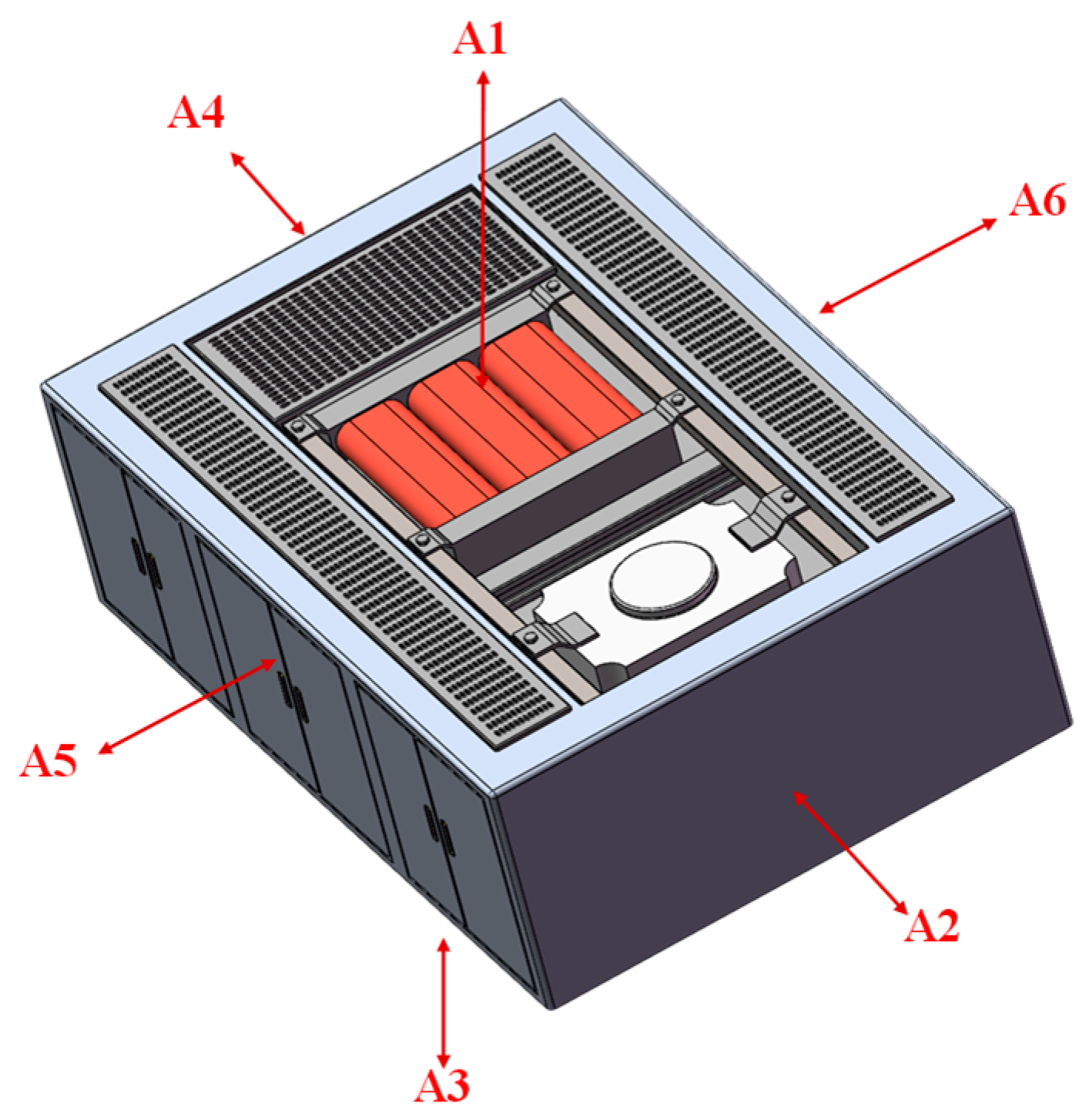
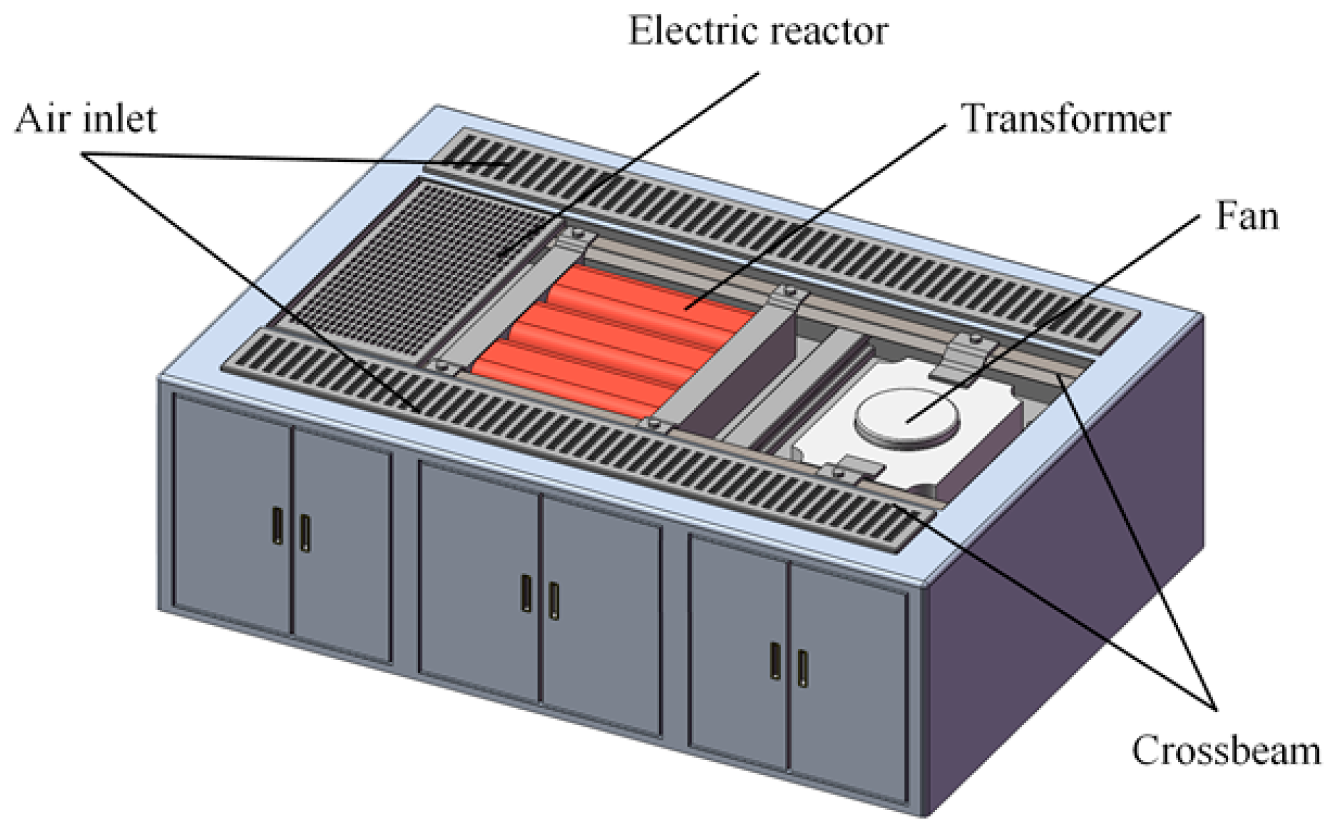
2.1. Converter Cabinet System

The converter cabinet mainly relies on the transformer, which uses the fan to dissipate heat, so the main noise sources are transformers and fans. The fan and transformer in the converter cabinet need to be operational at the same time, and the fan air duct must enter from both sides and exit through the transformer from the middle. The air outlet is right under the electric reactor. Figure 1 depicts the converter cabinet’s structural layout. The transformer is suspended on the left and right crossbeams through four rigid lifting eyes, and the fan is suspended on the same crossbeams through two rigid lifting eyes. The fan base is also connected to the bottom plate through four bolt holes. Zoom in on these installation locations in Figure 1, and as shown in Figure 2, the bolted connect locations between the converter cabinet, transformer, and fan are indicated by numbers 1 through 10.

By analyzing the working principle and structural characteristics of the converter cabinet, the following main noise sources are identified. The fan produces strong eddy current noise while rotating, as well as flow noise at the flow channel’s corners and variable cross-section, which is primarily transmitted from the air channel’s inlet and outlet. Under the influence of an electromagnetic field, the transformer body produces electromagnetic force, which stimulates it to produce loud noise. The entire cabinet vibrates and emits noise when the transformer is operating owing to the magnetostrictive effect of the silicon steel sheet material used in the construction of the transformer, which is transmitted to the cabinet system through the bolt installation point. The fan vibrates when it is operating because it is periodically struck by airflow. This vibration is then transmitted to the cabinet’s equipment via the bolts holding the fan in place, which increases cabinet vibration and emits noise.

According to the different transmission path, the noise of the transformer and fan to the target point is divided into two categories: structural noise and air noise. When the transformer and fan work, they vibrate themselves and transmit vibration to the whole cabinet through their respective connected structures (beams and baseboards), and they radiate noise from the cabinet to the target point. The noise radiated by the vibration of the shell of the transformer and the fan during work or the aerodynamic noise generated during work is transmitted to the evaluation point through the flow channel or leaks from the structural gap to the target point, or it is transmitted from the cabinet wall panel to the target point (due to the strong sound insulation ability of the wall panel, the transmitted part can be ignored).

2.2. Transfer Path Analysis Method

The primary objective of transmission path analysis is to reduce the complexity of the system into an analysis model of incentive source transmission path target point. By analyzing the contribution of the excitation source transmitted to the designated target point, the main sound source can be located, giving instructions for system noise control. The noise sound pressure or vibration level at the target point is equal to the sum of the energy propagated along various paths to the evaluation point by each excitation source under working load excitation, assuming that the entire converter cabinet system is linearly invariant. When considering both structural sound and airborne sound, the target point noise can be expressed as

$$P_l\left(t\right)=\sum _{i=1}^u P_{li}\left(t\right)+\sum _{j=1}^v P_{lj}\left(t\right)$$

(1)

The number of transmission paths for the structural and acoustic loads, respectively, are indicated by $u$ and $v$ in the equation. $P_l\left(t\right)$ is the total contribution response of the $l$-th target point; $t$ is a time variable; $P_{li}\left(t\right)$ is the contribution of the structural load of the i-th path to the target point l; $P_{lj}\left(t\right)$ is the contribution of the air load of the j-th path to the target point l.

Through the reference point signal and the transfer function from the path point to the reference point when the converter cabinet is working, the load at the path point when the converter cabinet is working can be obtained by using the inverse matrix method.

$$\left[\begin{array}{c}{F}_1\\ ⋮\\ F_n\end{array}\right]={\left[\begin{array}{cccc}{H}_{X_1/F_1}& H_{X_1/F_2}& \dots & H_{X_1/F_n}\\ ⋮& ⋮& \ddots & ⋮\\ H_{X_m/F_1}& H_{X_m/F_2}& \dots & H_{X_m/F_n}\end{array}\right]}^{-1}\left[\begin{array}{c}{a}_1\\ ⋮\\ a_m\end{array}\right]$$

(2)

which can be simplified as

$${\left[F\right]}_n={{\left[H\right]}^{-1}}_{m\times n}{\left[a\right]}_m$$

(3)

The term m in the equation represents the number of reference points, and n represents the number of path points. ${\left[F\right]}_n$ represents the load at the path point. Term ${\left[H\right]}_{m\times n}$ is the transfer function matrix from the path point to the reference points. Term $a_m$ represents the acceleration response of the reference point during operation.

The number of reference points m (m = 26) and path points n (n = 13) tested satisfy the matrix statically indeterminate condition: $m\ge 2n$, ensuring sufficient accuracy when solving the inverse matrix. ${\left[H\right]}_{m\times n}^{-1}=\left({\left[H\right]}^T\right[H]{)}^{-1}{\left[H\right]}^T$ is created when $m>n$ and takes the place of ${\left[H\right]}_{m\times n}^{-1}$. Singular value decomposition (SVD) for $\left[H\right]$, which is transformed into orthogonal space through SVD, is performed concurrently in order to prevent calculation errors brought on by improperly conditioned matrices. Different singular values and singular vectors in the system matrix represent various linear independences or independent terms. Utilizing LMS TPA software (Siemens LMS Test.Lab 17A), perform SVD decomposition on the frequency response function matrix to determine the load at the working path point based on the measured data. The target point response is calculated by calculating the load at the path point and the transfer function from the path point to the target point.

$$\left[\begin{array}{c}{P}_1\\ ⋮\\ P_q\end{array}\right]=\left[\begin{array}{cccc}{H}_{P_1/F_1}& H_{P_1/F_2}& \dots & H_{P_1/F_n}\\ ⋮& ⋮& \ddots & ⋮\\ H_{P_q/F_1}& H_{P_q/F_2}& \dots & H_{P_q/F_n}\end{array}\right]\left[\begin{array}{c}{F}_1\\ ⋮\\ F_n\end{array}\right]$$

(4)

simplified as

$${\left[P\right]}_q={\left[H\right]}_{q\times n}{\left[F\right]}_n$$

(5)

where term $q$ in the equation represents the number of target points; the term ${\left[P\right]}_q$ represents the sound pressure at each target point; the term ${\left[H\right]}_{q\times n}$ refers to the transfer function matrix from the path point to the target point.

3. Transfer Path Analysis Test

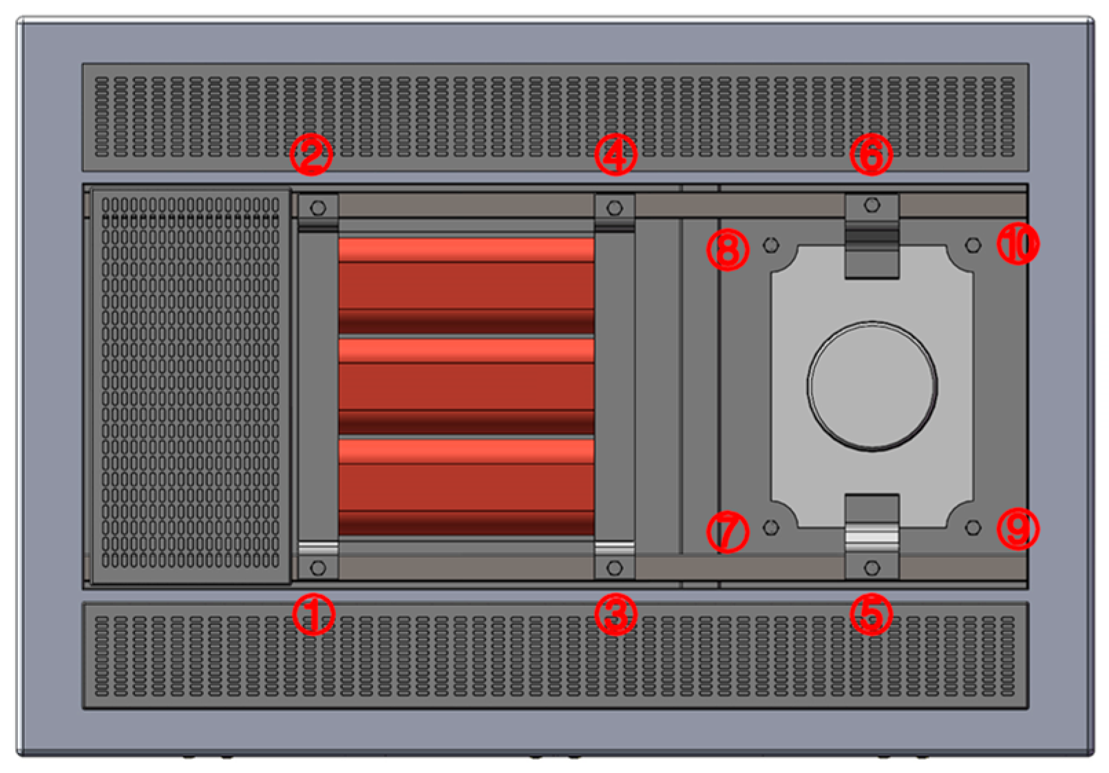
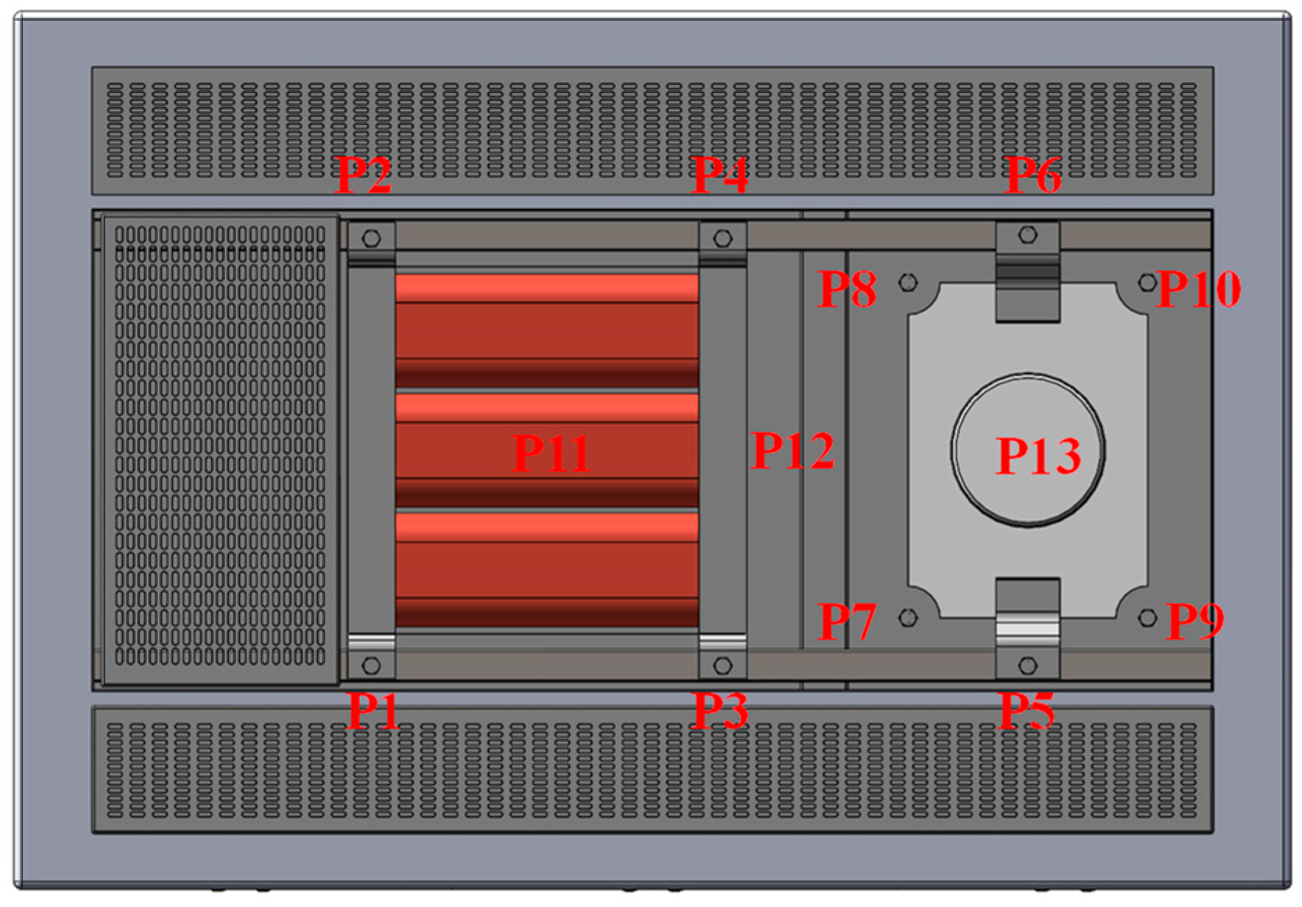
3.1. Testing Arrangement

The test mainly collects the vibration and noise signal and transfer function of the flow cabinet in different states and working conditions and analyzes the vibration and noise transmission characteristics of the transformer under test by using the transmission path. Position the microphone and accelerometer as described below, connect the data acquisition system (LMS. Test. Lab 17A, 24 channels) to the laptop computer, use the sampling analyzer FFT for spectrum analysis, and use the time recorder to record the time domain data. The sound excitation source is provided by LMS Company (Louvain, Belgium), model E-MVVFS. The main test contents are shown in

Table 1. Test content.

Test Type	Test Content		Remark
Working signal	The noise or vibration signals of I1b-I13a and A1–A6 points are collected under four working conditions		The signal is collected three times for each working condition, and the average value is obtained.
Transfer function	force-sound	I1b-I13a was excited, respectively, and P1–P13 signals were collected	The signal was measured three times for each excitation point and averaged.
	sound-sound	I1b-I13a was excited, respectively, and P1–P13 signals were collected

.

When the converter is not working, a microphone is used to test the background noise on the surface of the converter body. The test environmental conditions require the background noise level (SPL) to be low enough. Generally speaking, the difference between the background noise and the total noise of the test object sound source is less than 3 dB (A), so the measurement is not accurate. It needs to be corrected to between 3 and 10 dB (A). When the noise of the tested object is more than 10 dB (A) higher than the background noise, the result does not need to be corrected. Install the inverter cabinet on the test bench during a quiet period (when there is no activity or little noise impact in the traction test room). The background noise at each measurement point is more than 10 dB (A) lower than the test noise, which can be seen through noise testing to be 14.88 dB (A) on average. The test results do not need to be corrected. Through the above analysis, n theoretical transfer paths (n = 13) can be analyzed according to the structural characteristics and source characteristics of the transformer tank of the test object. According to the general requirements of the TPA theory above, 26 reference points are arranged in the test scheme. Figure 3 and Figure 4 depict the measurement point layout, and the layout form is as follows. Six target spots are designated A1 through A6, each 0.8 m from the cabinet’s surface; the 13 path points are designated P1–P13. Six vibration points are among them and each are transmitted twice along the beam, in the Z and X directions, with little or no effect in the Y direction, which is the beam’s axial direction. Three of the four places on the fan’s suspension system that convey vibration in one direction are air noise path points. The bottom air outlet is where P13 is located; to gather surface normal acceleration data, there are 26 reference points labeled I1a, I1b–I13a, and I13b, which are all positioned on the left or right sides of the 13 path points.

3.2. Testing Procedure

During the actual operation of the converter, the fan must run continuously to dissipate heat from the transformer; therefore, only two representative operating conditions—full speed and half speed—are used to determine the vibration and noise characteristics of a single fan. This serves as the basis for testing the transformer’s vibration and noise characteristics under complex working conditions with half load and full load. The working condition data are then measured. Close the cover plate of the converter cabinet and operate the converter cabinet according to the working conditions. Measure the noise and vibration responses of target points and reference points. The reference point signal is used to calculate the path load, and each working condition is measured 3 times. The test conditions are shown in

Table 2. Test conditions.

Condition Number	Condition State
1	Fan at half speed and transformer at no-load
2	Fan at full speed and transformer at no-load
3	Fan at half speed and transformer at full load
4	Fan at full speed and transformer at full load

.

(1)

Working condition data measurement. Close the upper end of the cover plate of the converter cabinet, and operate the converter cabinet according to the requirements of the four working conditions in Table 2 under normal operation. The noise and vibration response of the target point and reference point are measured. The reference point signal is used to calculate the path load. Each working condition is measured 3 times. The test conditions are shown in Table 2.

(2)

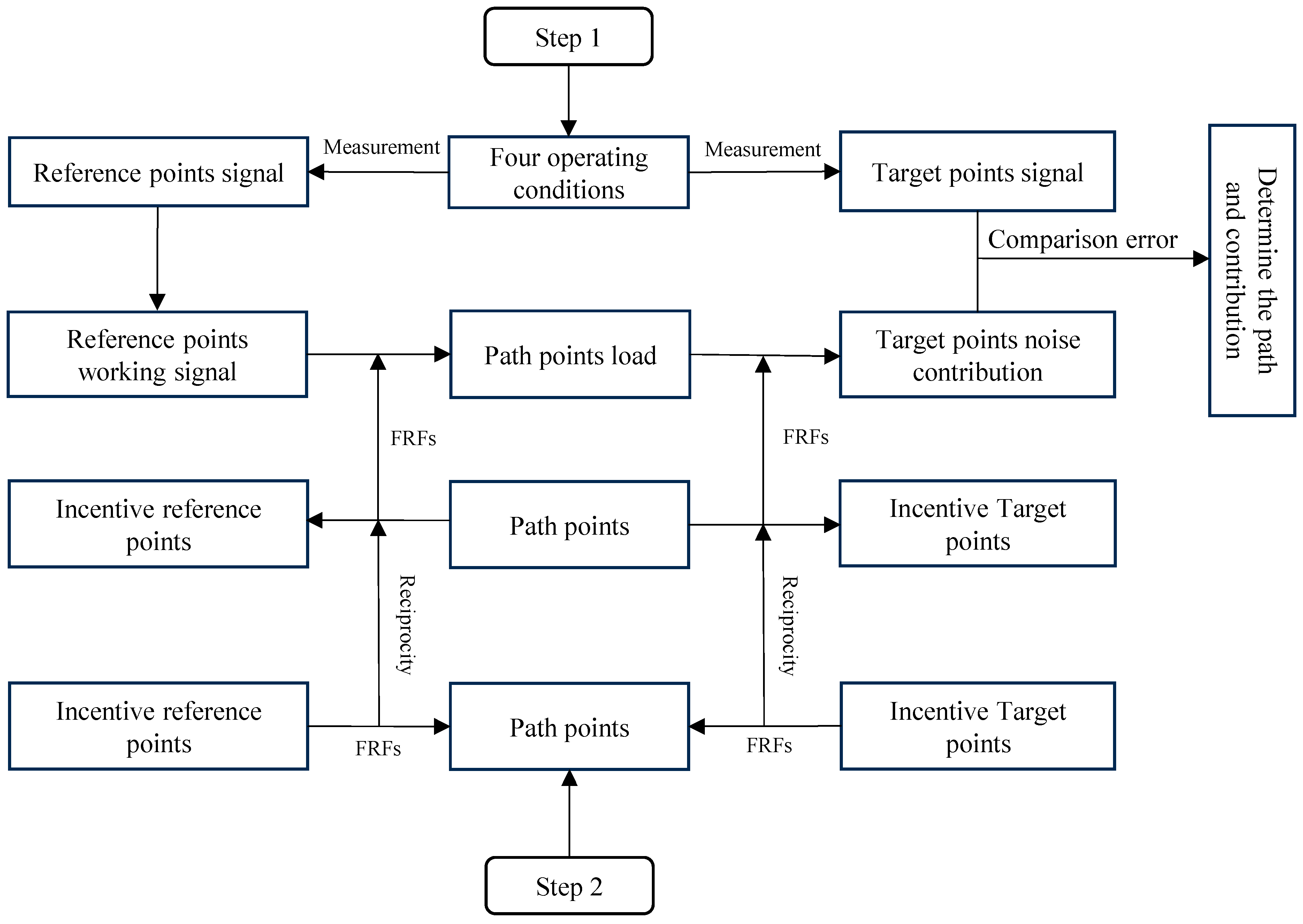
Transfer function measurement. The reciprocity principle reveals the reciprocity between vibration and sound transmission in a linear time-invariant elastic system, that is, the ratio of an incentive applied at one point A in the system to the response generated by that incentive at another point B in the system is equal to the ratio of an incentive applied at B to the response generated at A. Due to the complexity of the structure of the measured object and the limited internal space structure, it is difficult to directly test the response of the reference point and the target point, respectively, with the excitation path points. The transfer function is an inherent attribute of the structure and does not change with the excitation force, so the reciprocity method is used for measurement. Remove the converter cabinet and fan, close the cover plate, open a hole in the cover plate to lead out the sensor cable, and seal it with mastic. Firstly, the reference point is stimulated by a hard hammer, the response of the internal path is measured, and the transfer function from the reference point to the path point is obtained. Then, the volume sound source excites the external target point, measures the response of the internal path, and obtains the transfer function from the target point to the internal path. At this point, the transfer function between the reference point, the path point, and the target point can be obtained and the contribution can be solved. The test procedure is shown in Figure 5.

4. Noise Source Diagnosis by TPA-NN

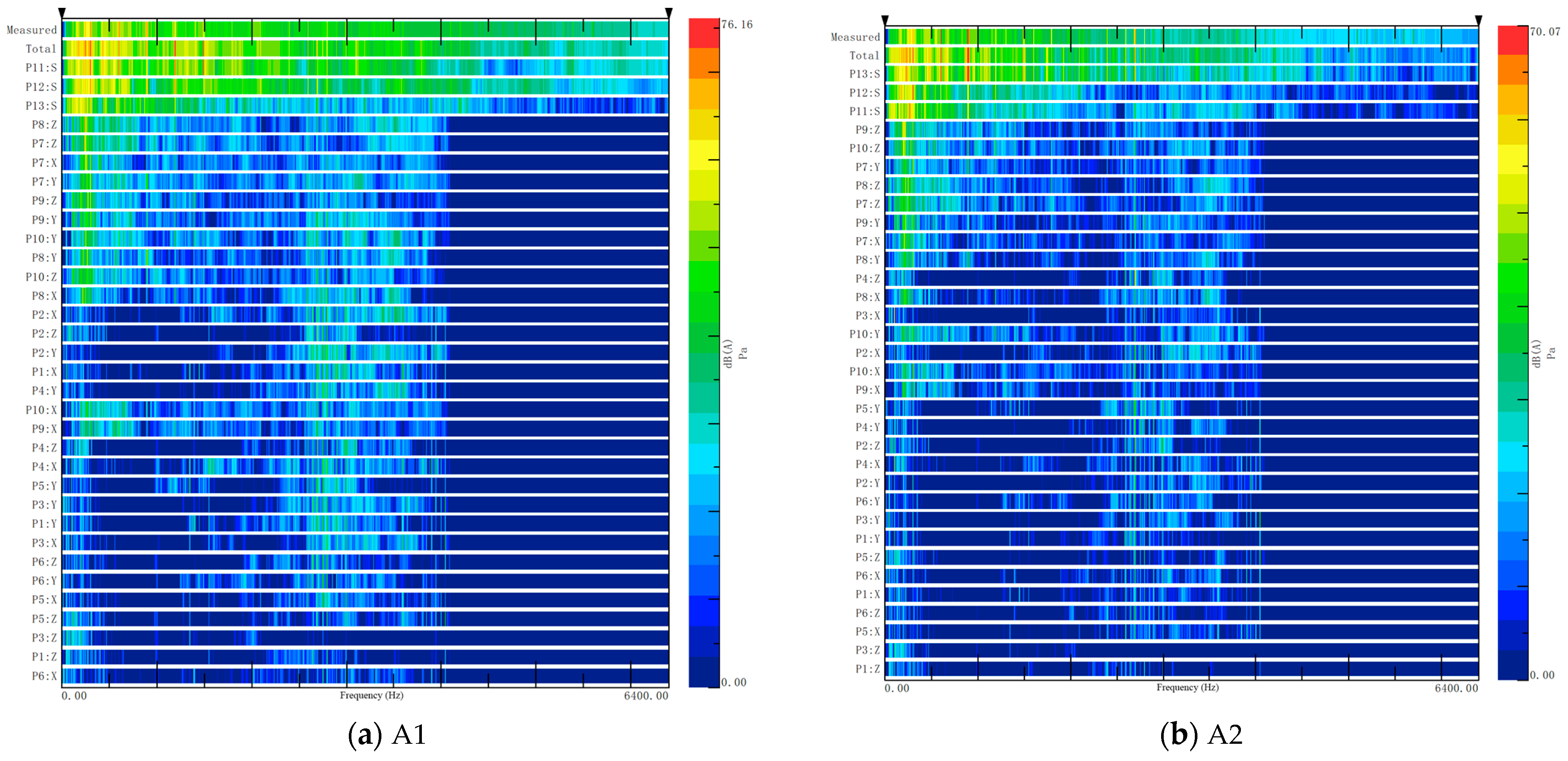
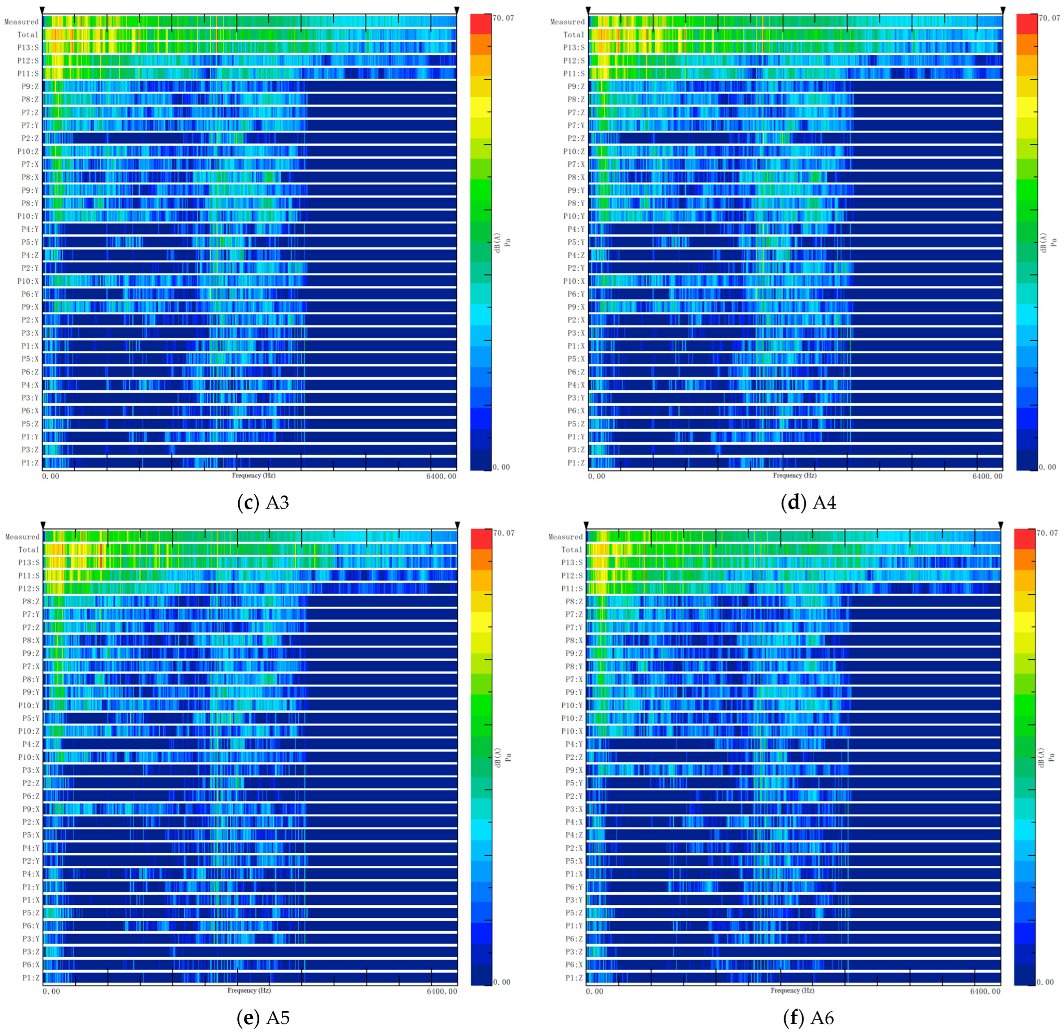
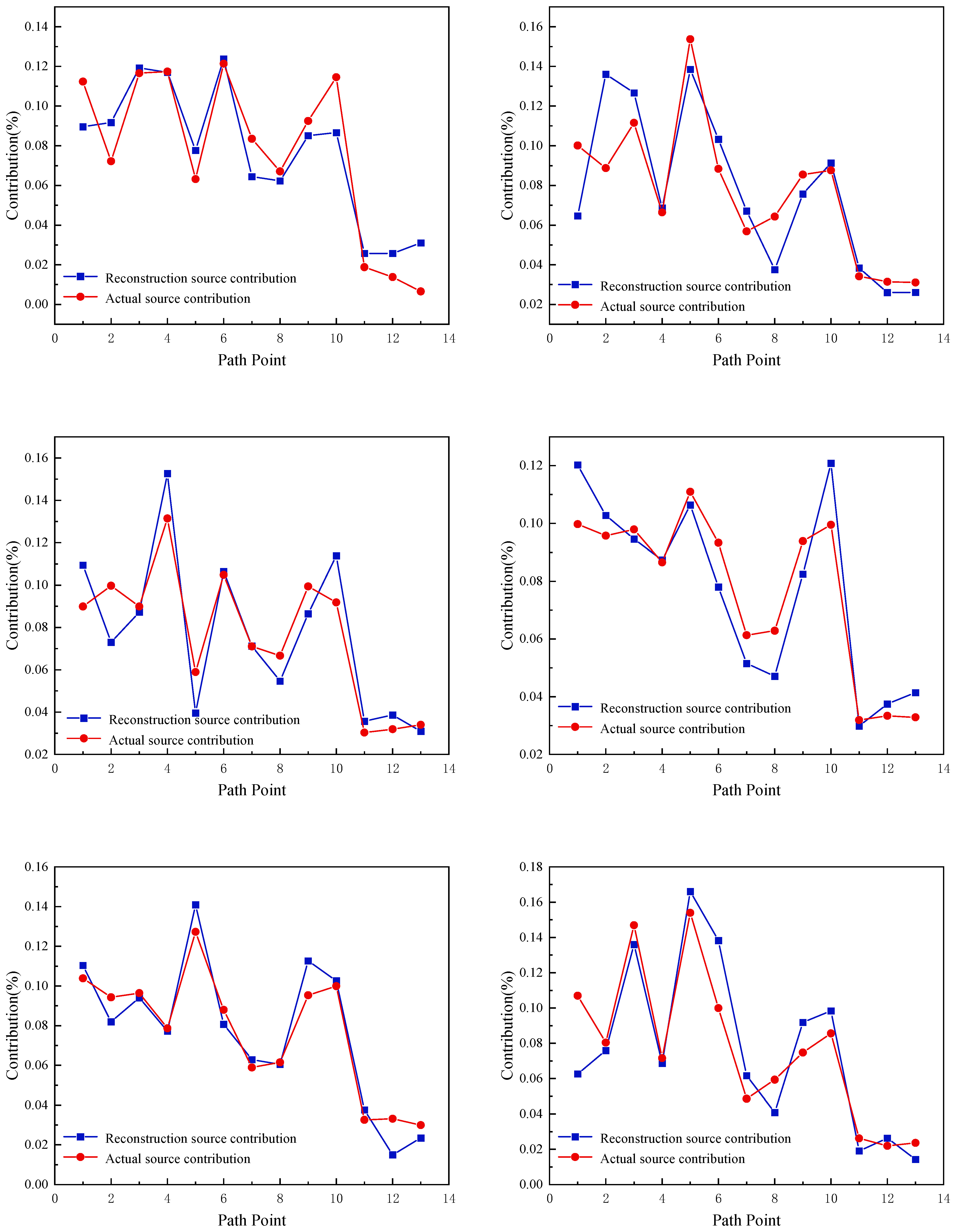
4.1. Sound Source Contribution Analysis Based on TPA Test

According to the calculated path load and the transfer function from the path to the target point, the synthesized noise at the target point A3 can be obtained using LMS TPA software. At the same time, the microphone was used to test the actual noise data at point A3 under the same working condition. As shown in Figure 6, the synthetic noise was basically consistent with the test noise in the entire frequency range, which characterized the rationality of the TPA model. The A3 point contribution chromatography is shown in Figure 7.

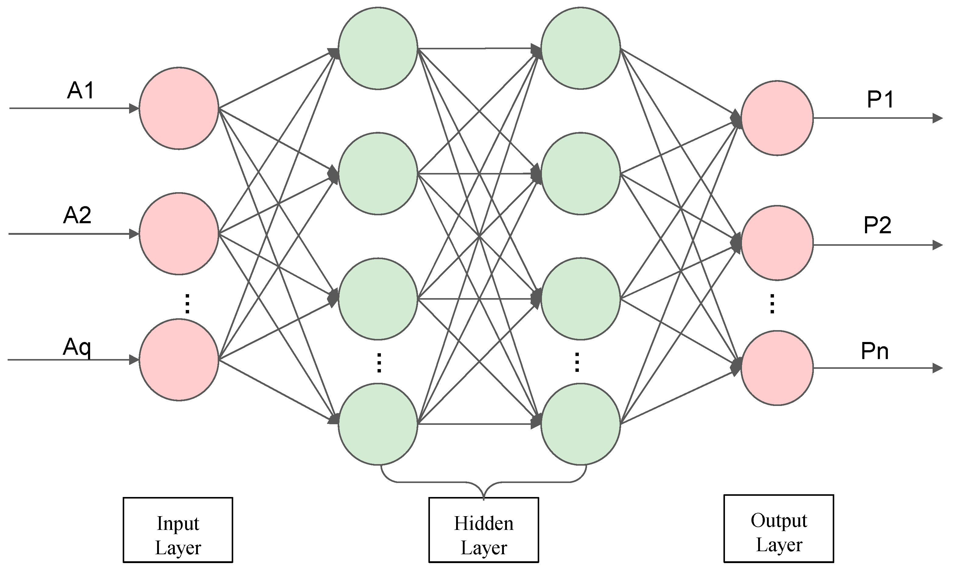
4.2. Network Structure

The contribution of the path point is inversely solved by the transfer function from the path point to the target point through the response of the target point when working in the converter cabinet. Simultaneously, the unknown contribution is 13 and the known response is 6. According to the mathematical analysis, when the unknown is greater than the number of equations, the solution of the path contribution is not unique. Taking the above target point response as the input and path contribution as the output of the neural network, the network structure in this paper is determined by comparison and parameter adjustment, as shown in Figure 8. Among them, red represents the input/output layer, and green represents the hidden layer.

The network consists of one input layer, two hidden layers for a fully connected layer, and one output layer. Fully connected layer operations are essentially linear transformations from one feature space to another. Unlike convolutional networks that extract local features, each fully connected layer neuron can be treated as a polynomial that optimizes the weight coefficient through backpropagation to obtain the appropriate weight, and extracts global features through the weight matrix.

The upper limit of transformer electromagnetic noise is about 6000 Hz, and in order to avoid data omission, the upper limit of test data is raised to 10,240 Hz. The input layer receives a two-dimensional array of the shape (10240,6), i.e., six target points in the range of 0–10,240 Hz, through the first fully connected layer, which has six neurons and applies the ReLU activation function to extract the input features; through the second fully connected layer, which has nine neurons, and the ReLU activation function is applied to further capture the relevant features in the input data; and finally, through the output layer to obtain the contribution of each path to the target point. The output layer has 13 neurons, and the Softmax activation function is applied, which converts the real value vector of the output from the previous layer into a normalized probability distribution, which is the normalized output, and the sum of the outputs is equal to 1.

The activation function expression is as follows:

$$ReLu=\max \left(0,x\right)$$

(6)

$$Softmax=\frac{e^{z_i}}{{\sum }_{j=1}^K{e}^{z_j}}$$

(7)

where $Z_i$ is an element of the input vector of the function, ${\sum }_{j=1}^K{e}^{z_j}$ is a normalized term. Equation (7) ensures that all output values of the function add up to 1, and that each value is in the range (0, 1), thus constituting a valid probability distribution, where $K$ is the generic number.

To train and optimize the model, the optimizer Nadam (Nesterov-accelerated Adaptive Emoment Estimation) is selected, and the Mean Squared Error MSE (Mean Squared Error) is used as the loss function of the model. Minimize the difference between the model output and the real output so that the model can accurately predict the desired output.

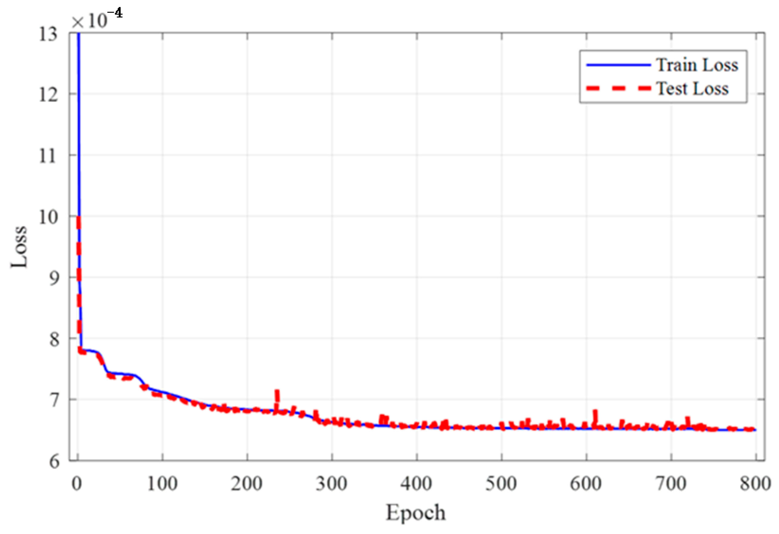
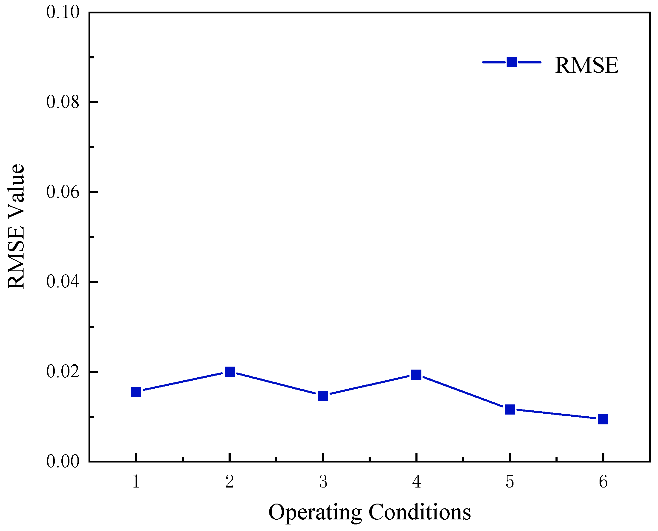
4.3. Network Training and Results

The spectrum data of the actual contribution obtained through the forward solution of the test are sent to the neural network as data samples for training as shown in Figure 9. The data sample is divided into the training set and the test set in an 8:2 ratio. The training batch size was 64 and the training batch epochs was 800 rounds. The training loss and test loss curves of the TPA-NN model are shown in the figure. It can be seen from the figure that both training loss and verification loss decrease continuously with the increase in training rounds, and the curves fit well. Finally, both training loss and test loss approach 6 × 10⁻⁴. As a result, the TPA-NN model’s training and verification effects might be regarded as positive.

In order to verify the accuracy of the network output results, six groups of target points outside the data samples were randomly selected to inversely solve 13 path point contributions in the test data with a frequency of 50 Hz. The comparison between the neural network reconstruction contribution and the actual contribution is shown in Figure 10. The comparison between the actual contribution and the reconstruction contribution of 13 paths that correspond to the six target points is displayed in six subgraphs. Figure 11 indicates the root mean square error between the reconstructed contribution and the actual contribution of six randomly selected target points’ test data. The error does not exceed 0.02, indicating that this method has high accuracy and meets practical engineering needs. The overall trend observation reveals that the contribution of the reconstruction path of the six target points is basically consistent with the actual contribution, indicating the reliability of this method in reverse solving the contribution during the actual operation of the converter cabinet.

5. Conclusions

According to the structure of the converter, the characteristics of the sound source and noise transmission path of the converter are analyzed, and the traditional TPA test scheme is designed. The data of four working conditions are tested, and the transfer function matrix of each path point’s contribution to the target point is obtained. The actual contribution of each path to the target point is calculated. In order to solve the inverse ill-posed problem when the target points are smaller than the path points, the inverse reconstruction method of TPA-NN, which combines the traditional TPA test scheme and neural network, is proposed. In order to verify the accuracy of the proposed method, the path point contribution at some frequencies is reconstructed. The results show that when the path point number of the converter is 13 and the target point number is 6, the root-mean-square error between the reconstructed contribution and the actual contribution is less than 0.02, and the results of the proposed method are more accurate.

In future work, we will continue to promote the versatility and accuracy of TPA-NN methods, including the combination of other types of TPA methods with neural networks and the improvement of neural network structures, such as the introduction of one-dimensional convolutional networks, to improve the accuracy of this method.

References

1. Guo, R.; Qiu, S.; Yu, Q.L.; Zhou, H.; Zhang, L.J. Transfer path analysis and control of vehicle structure-borne noise induced by the powertrain. Proc. Inst. Mech. Eng. Part D-J. Automob. Eng. 2012, 226, 1100–1109. [Google Scholar] [CrossRef]
2. Xu, Z.; Wei, J.; Zhang, S.; Liu, Z.; Chen, X.; Yan, Q.; Guo, J. A state-of-the-art review of the vibration and noise of wind turbine drivetrains. Sustain. Energy Technol. Assess. 2021, 48, 101629. [Google Scholar] [CrossRef]
3. Plunt, J. Finding and Fixing Vehicle NVH Problems with Transfer Path Analysis. Sound Vib. 2005, 39, 12–17. [Google Scholar] [CrossRef]
4. Diez-Ibarbia, A.; Battarra, M.; Palenzuela, J.; Cervantes, G.; Walsh, S.; De-La-Cruz, M.; Theodossiades, S.; Gagliardini, L. Comparison between transfer path analysis methods on an electric vehicle. Appl. Acoust. 2017, 118, 83–101. [Google Scholar] [CrossRef]
5. Klerk, D.D.; Ossipov, A. Operational transfer path analysis: Theory, guidelines and tire noise application. Mech. Syst. Signal Process. 2010, 24, 1950–1962. [Google Scholar] [CrossRef]
6. Sitter, G.D.; Devriendt, C.; Guillaume, P.; Pruyt, E. Operational transfer path analysis. Mech. Syst. Signal Process. 2010, 24, 416–431. [Google Scholar] [CrossRef]
7. Janssens, K.; Gajdatsy, P.; Gielen, L.; Mas, P.; Britte, L.; Desmet, W.; Van der Auweraer, H. OPAX: A new transfer path analysis method based on parametric load models. Mech. Syst. Signal Process. 2011, 25, 1321–1338. [Google Scholar] [CrossRef]
8. Tosun, M.; Yildlz, M.; Ozkan, A. Investigation and refinement of gearbox whine noise. Appl. Acoust. 2018, 130, 305–311. [Google Scholar] [CrossRef]
9. Wang, Z.W.; Zhu, P.; Shen, Y.; Huang, Y.Y. An improved OPAX method based on moving multi-band model. Mech. Syst. Signal Process. 2019, 122, 321–341. [Google Scholar] [CrossRef]
10. Cheng, W.; Blamaud, D.; Chu, Y.; Meng, L.; Lu, J.; Basit, W.A. Transfer Path Analysis and Contribution Evaluation Using SVD- and PCA-Based Operational Transfer Path Analysis. Shock Vib. 2020, 2020, 9673838. [Google Scholar] [CrossRef]
11. Zhu, P.; Wang, Z.; Qin, Z.; Shen, Y. The transfer path analysis method on the use of artificial excitation: Numerical and experimental studies. Appl. Acoust. 2018, 136, 102–112. [Google Scholar] [CrossRef]
12. Ye, S.; Hou, L.; Zhang, P.; Bu, X.; Xiang, J.; Tang, H.; Lin, J. Transfer path analysis and its application in low-frequency vibration reduction of steering wheel of a passenger vehicle. Appl. Acoust. 2020, 157, 107021. [Google Scholar] [CrossRef]
13. Gajdatsy, P.; Janssens, K.; Desmet, W.; Van der Auweraer, H. Application of the transmissibility concept in transfer path analysis. Mech. Syst. Signal Process. 2010, 24, 1963–1976. [Google Scholar] [CrossRef]
14. Tang, Z.; Zan, M.; Zhang, Z.; Xu, Z.; Xu, E. Operational transfer path analysis with regularized total least-squares method. J Sound Vib. 2022, 535, 117130. [Google Scholar] [CrossRef]
15. Ström, R. Operational Transfer Path Analysis of Components of a High-Speed Train Bogie. Master’s Thesis, Chalmers University of Technology, Gothenburg, Sweden, 2015. [Google Scholar] [CrossRef]
16. Wang, J.; Yang, M.Q.; Liang, F.; Feng, K.R.; Zhang, K.; Wang, Q. An Algorithm for Painting Large Objects Based on a Nine-Axis UR5 Robotic Manipulator. Appl. Sci. 2022, 12, 7219. [Google Scholar] [CrossRef]
17. An, K.; Lee, S.-K. Identification of Influence of Cross Coupling on Transfer Path Analysis Based on OPAX and OTPA in a Dummy Car. Int. J. Automot. Technol. 2021, 22, 771–778. [Google Scholar] [CrossRef]
18. Chen, K.; Zhang, X.; Liu, Y.; Ma, J. An improved denoise method based on EEMD and optimal wavelet threshold for model building of OPAX. Proc. Inst. Mech. Eng. Part D-J. Automob. Eng. 2021, 235, 3530–3544. [Google Scholar] [CrossRef]
19. Rao, M.V.; Moorthy, S.N.; Raghavendran, P. Dynamic Stiffness Estimation of Elastomeric Mounts Using OPAX in an AWD Monocoque SUV; SAE Technical Paper 2015-01-2190; SAE International: Warrendale PA, USA, 2015; Volume 2190. [Google Scholar] [CrossRef]
20. Vincent, P.; Larochelle, H.; Lajoie, I.; Bengio, Y.; Manzagol, P.-A. Stacked Denoising Autoencoders: Learning Useful Representations in a Deep Network with a Local Denoising Criterion. J. Mach. Learn. Res. 2010, 11, 3371–3408. [Google Scholar]
21. Schmidhuber, J. Deep learning in neural networks: An overview. Neural Netw. 2015, 61, 85–117. [Google Scholar] [CrossRef]
22. Badrinarayanan, V.; Kendall, A.; Cipolla, R. SegNet: A Deep Convolutional Encoder-Decoder Architecture for Image Segmentation. IEEE Trans. Pattern Anal. Mach. Intell. 2017, 39, 2481–2495. [Google Scholar] [CrossRef]
23. Krizhevsky, A.; Sutskever, I.; Hinton, G.E. ImageNet Classification with Deep Convolutional Neural Networks. Commun. Acm. 2017, 60, 84–90. [Google Scholar] [CrossRef]
24. He, K.; Gkioxari, G.; Dollar, P.; Girshick, R. Mask R-CNN. IEEE Trans. Pattern Anal. Mach. Intell. 2020, 42, 386–397. [Google Scholar] [CrossRef]
25. Jain, M.; Kumar, A.; Bahl, R. Simulation-Based Asymptotic Study of Multi-channel Filtered-x Least Mean Square (MC-FxLMS) Algorithm for Active Noise Control. J. Vib. Eng. Technol. 2023, 11, 647–665. [Google Scholar] [CrossRef]
26. Zhang, D.; Zhong, Z.; Xia, Y.; Wang, Z.; Xiong, W. An Automatic Classification System for Environmental Sound in Smart Cities. Sensors 2023, 23, 6823. [Google Scholar] [CrossRef]
27. Zhou, M.; Han, J.; Rachh, M.; Borges, C. A neural network warm-start approach for the inverse acoustic obstacle scattering problem. J. Comput. Phys. 2023, 490, 112341. [Google Scholar] [CrossRef]
28. Salamon, J.; Bello, J.P. Deep Convolutional Neural Networks and Data Augmentation for Environmental Sound Classification. IEEE Signal Process. Lett. 2017, 24, 279–283. [Google Scholar] [CrossRef]
29. Van-Sang, D.; Thien, H.-T.; Kim, D.-S. Underwater Acoustic Target Classification Based on Dense Convolutional Neural Network. IEEE Geosci. Remote Sens. Lett. 2022, 19, 1500905. [Google Scholar] [CrossRef]
30. Cakir, E.; Parascandolo, G.; Heittola, T.; Huttunen, H.; Virtanen, T. Convolutional Recurrent Neural Networks for Polyphonic Sound Event Detection. IEEE-Acm. Trans. Audio Speech Lang. Process. 2017, 25, 1291–1303. [Google Scholar] [CrossRef]
31. Deng, M.; Meng, T.; Cao, J.; Wang, S.; Zhang, J.; Fan, H. Heart sound classification based on improved MFCC features and convolutional recurrent neural networks. Neural Netw. 2020, 130, 22–32. [Google Scholar] [CrossRef]
32. Seki, S.; Kameoka, H.; Li, L.; Toda, T.; Takeda, K. Underdetermined Source Separation Based on Generalized Multichannel Variational Autoencoder. IEEE Access 2019, 7, 168104–168115. [Google Scholar] [CrossRef]
33. Cody, R.A.; Tolson, B.A.; Orchard, J. Detecting Leaks in Water Distribution Pipes Using a Deep Autoencoder and Hydroacoustic Spectrograms. J. Comput. Civ. Eng. 2020, 34, 04020001. [Google Scholar] [CrossRef]
Figure 1. Schematic diagram of the converter cabinet structure.
Applsci 13 12244 g001
Figure 2. Partial enlarged view of installation site.
Applsci 13 12244 g002
Figure 3. Schematic diagram of target point layout.
Applsci 13 12244 g003
Figure 4. Layout plan of path points.
Applsci 13 12244 g004
Figure 5. Test steps.
Applsci 13 12244 g005
Figure 6. Comparison of test noise and synthetic noise.
Applsci 13 12244 g006
Figure 7. Target point contribution chromatography.
Applsci 13 12244 g007aApplsci 13 12244 g007b
Figure 8. Neural network structure diagram.
Applsci 13 12244 g008
Figure 9. Training and testing loss of TPA-NN.
Applsci 13 12244 g009
Figure 10. Comparison of theoretical and reconstructed source contributions.
Applsci 13 12244 g010
Figure 11. RMSE between actual contribution and reconstructed contribution.
Applsci 13 12244 g011