Adaptive Smoothing for Visual Improvement of Image Quality via the p(x)-Laplacian Operator Effects of the p(x)-Laplacian Smoothing Operator on Digital Image Restoration: Contribution to an Adaptive Control Criterion

Abstract

This article concerns the improvement of digital image quality using mathematical tools such as nonlinear partial differential operators. In this paper, to perform smoothing on digital images, we propose to use the p(x)-Laplacian operator. Its smoothing power plays a main role in the restoration process. This enables us to dynamically process certain areas of an image. We used a mathematical model of image regularisation that is described by a nonlinear diffusion Equation (this diffusion is modelled by the p(x)-Laplacian operator). We implemented the continuous model in order to observe the steps of the regularisation process to understand the effects of the different parameters of the model on an image. This will enable parameters to be used and adapted in order to provide a proposed solution.

1. Introduction

The smoothing of digital images is an important theme in the field of image correction. It provides a method for erasing unwanted effects caused by various factors, such as the quality of the acquisition material, human error or the degradation induced in order to reduce its storage space.

There are many processing operators for smoothing digital images. Their aim is to maintain highlights in the relevant areas and smooth the rest.

Among these operators, we can mention the p(x)-Laplacian operator, which mathematically models the diffusion of a signal (in this case, a digital image), taking into account the local information of this signal. This operator, by its formulation, is able to perform smoothing according to a criterion. Generally, in the literature, the criterion defining the degree of smoothing for the p(x)-Laplacian operator is calculated at the beginning of processing. In this way, the amount of smoothing is set to the same level. In the present work, contrary to what is generally carried out, we wanted to make the processing adaptive by locally adjusting the criterion taken into account in the definition of the p(x)-Laplacian operator. Thus, this procedure allows us to select, from the observed image, the areas that will undergo the necessary smoothing while preserving those that we consider more important.

In recent years, the most common version is the lossy compression, which often results in image degradation. In this context, we propose the adaptation of a nonlinear mathematical model for the improvement of these images. Currently, most image restoration methods are based on partial differential Equations (see [1,2,3,4]) that involve two parameters, one of which is always considered to be fixed.

This paper is organised as follows:

• Section 1 introduces the subject matter of this work and the setting of the problem;
• In Section 2, we present the main mathematical tools associated with a continuous version of the problem and its formulation. The use of graph theory proposes a discretised version of the initial problem by employing an adaptive algorithm. In addition, we recall some current properties of the $p\left(x\right)$-Laplacian operator;
• Section 3 discusses the simulation approaches;
• Section 4 proposes some illustrations of usually referenced images which are provided in well-known databases;
• Section 5 addresses some comparative studies between our proposed approach and others.

2. Context and Problems

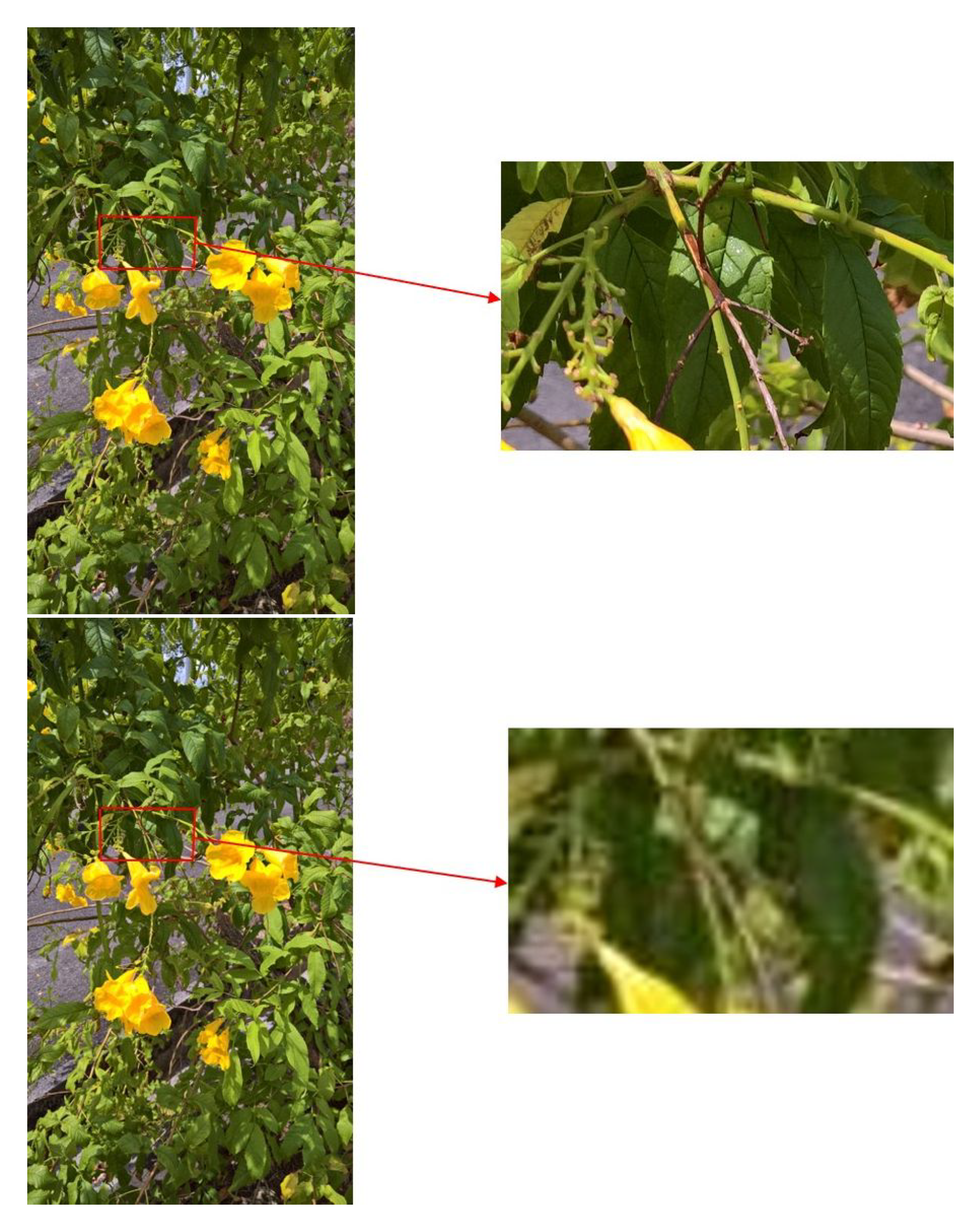
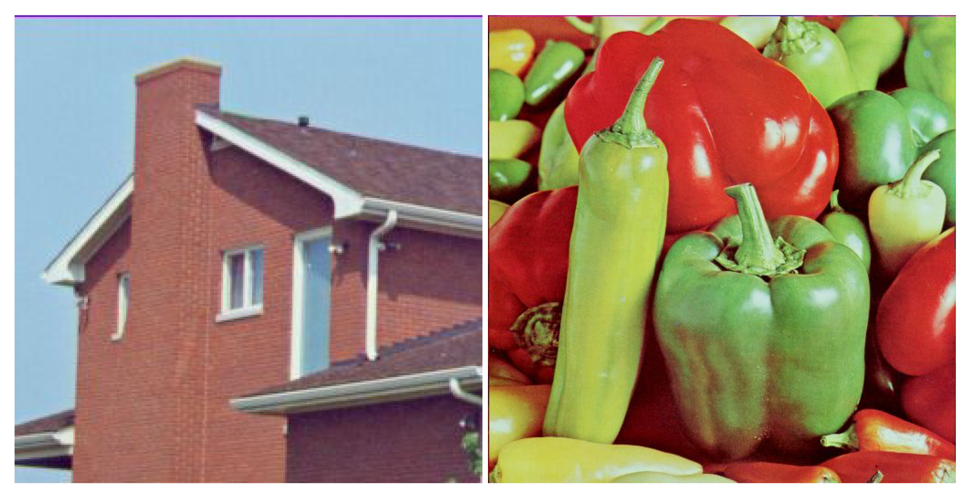
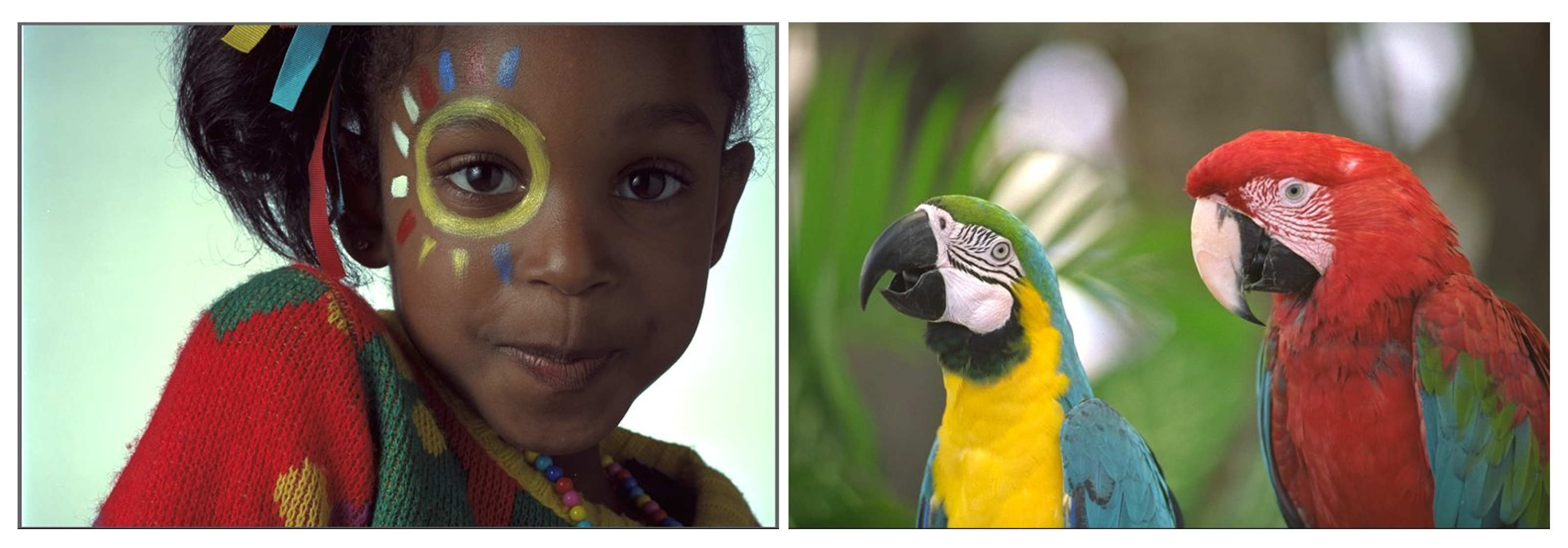
2.1. Pictures

Images may have minor changes that are in need of smoothing in order to improve their readability. The image shown in Figure 1 is an example of the type of degradation that can be seen in an image.

All equipment has sensors and acquisition algorithms that are more or less efficient, which means that quality is lost. To this, one must add the human factor [5], which is often the reason why the work of an inexperienced photographer has lower quality.

2.2. Adaptive Smoothing Using the p(x)-Laplacian

Mathematical modelling is used to model phenomena from various fields, including physics, chemistry, biology and, in particular, digital image processing. In some cases, computer science makes it possible to apply some of these patterns to improve the quality of digital images. In this paper, we use the results from a class governed by a nonlinear operator of the pseudo-Laplacian-type with a variable exponent. In our case, this function denotes an image (see [6]).

Our aim is to improve the quality of the images by homogenising areas where the gradient is low, while preserving the amount of detail in the areas where the gradient is high.

3. The Method

3.1. Presentation of Some Models with a Diffusion Term

First of all, we must consider that an observed digital image $f_0$ is the noisy image. This digital image could be interpreted as a real image f (the desired one) with one (or several) noise(s) or residual(s) of image r (see [7], p. 6, (18) r = N(0;$\sigma$) is considered as a Gaussian noise with mean = 0 and deviation $\sigma$). The effects of the degradation (caused by the camera or object motion, atmospheric turbulence optics, etc.) on the piecewise smooth image f are modelled by a linear or a nonlinear operator K. Usually, the operator K is named the degradation operator or degradation function, and it is also known as a point spread function (PSF) or kernel.

This is modelled by the following equation

$$f_0=K\left(f\right)+r.$$

(1)

The smoothing process consists of approaching $f$ from $f_0$ by means of a minimisation problem of the energy function $E(f;f_0;\lambda )$ as defined below

$$E(f,f_0,\lambda )=E_{reg}\left(f\right)+\lambda E_{approx}(f,f_0)$$

(2)

where

• $E(f;f_0;\lambda )$ stands for the energy that allows one to go from $f_0$ to the desired image;
• $E_{reg}\left(f\right)$ denotes the regularisation energy to the real image f;
• $E_{approx}(f,f_0)$ interprets the energy of approximation between the real image f and the observed image $f_0$, also named the fitting term or the fidelity term;
• $\lambda$ is the fidelity parameter or the penalty parameter.

The main goal is to recover an image corrupted by the noise while preserving edges and some details on the observed image and small scale structures such as textures and other details on the observed image.

Among examples of energies functions, we can cite the following continuous energies functions.

$$E(f,f_0,\lambda )={\int }_{\mathrm{\Omega }}\left|\nabla f\right|dx+\frac{\lambda }{2}{\int }_{\mathrm{\Omega }}{\left|f-f_0\right|}^{2}dx,$$

(3)

$$E(f,f_0,\lambda )={\int }_{\mathrm{\Omega }}{\left|\nabla f\right|}^{2}dx+\frac{\lambda }{2}{\int }_{\mathrm{\Omega }}{\left|f-f_0\right|}^{2}dx.$$

(4)

Models (3) and (4) were introduced by Rudin et al. in [3].

We can also cite the model associated with the following energy function

$$E(f,f_0,\lambda )={\int }_{\mathrm{\Omega }}{\left|\nabla f\right|}^{p\left(x\right)}dx+\frac{\lambda }{2}{\int }_{\mathrm{\Omega }}{\left|f-f_0\right|}^{2}dx.$$

(5)

here, the variable exponent p is defined as follows

$$p\left(x\right)=\left\{\begin{array}{cc}\hfill 1& \hfill \mathrm{if}\left|x\right|>M,\hfill \\ \hfill 2& \hfill \mathrm{if}x=0\hfill \end{array}\right.$$

where $M>0$ is a positive constant. Precisely, $M>0$ is either the index of the preservation (i.e., $\left|x\right|>M)$ or the index of degradation (i.e., $\left|x\right|\le M)$. For more details, a reader interested in the field can refer to [1].

A variant of Model (5) is the following

$$E(f,f_0,\epsilon )=\frac{1}{\epsilon }{\int }_{\left|\nabla f\left(x\right)\right|<\epsilon }{\left|\nabla f\right|}^{2}dx+\frac{1}{2\epsilon }{\int }_{\left|\nabla f\right|\ge \epsilon }\left(\left|\nabla f\right|-\frac{\epsilon }{2}\right)dx+\frac{\lambda }{2}{\int }_{\mathrm{\Omega }}{\left|f-f_0\right|}^{2}dx.$$

(6)

This energy function was introduced by Chambolle and Lions [2]. In this model, we can observe that $p=2$ for $\left|\nabla f\left(x\right)\right|<\epsilon$, while $p=1$ for $\left|\nabla f\left(x\right)\right|\ge \epsilon$.

3.2. The Formulation of the Present Model

To date, the previous models have been considered with a degree of smoothness p independent of the location x in the domain $\mathrm{\Omega }$. The aim of our paper is to observe the effects of the degree of smoothness depending on the location x. Taking into account the spatial location x, the smoothness is considered a dynamic process linked to the following energy function.

$$E(f,f_0,\lambda )={\int }_{\mathrm{\Omega }}\frac{1}{p\left(x\right)}{\left|\nabla f\right|}^{p\left(x\right)}dx+\frac{\lambda }{2}{\int }_{\mathrm{\Omega }}{\left|f-f_0\right|}^{2}dx$$

(7)

where

$$p\left(x\right)=1+\frac{1}{1+k{|\nabla G_{\sigma }\star f_0\left(x\right)|}^2},k,\sigma >0,$$

(8)

$G_{\sigma }\left(x\right)={\sigma }^{-1}exp\left(-{\left|x\right|}^2/4{\sigma }^2\right)$ represents the Gaussian filter function. Models (7)–(8) were suggested and investigated by Chen, Levine, and Rao in [4] in the special context of BV${}^p(·)$ functions. For more details and properties on BV${}^p(·)$ functions, an interested reader can consult [8].

The variable exponent function $p(·)$ belongs in the interval $[1;+\infty [$

 It represents a regularisation degree. It also improves the quality of the image resulting from the smoothing process. More precisely, this function encodes the information on the regions where the gradient is near zero (the homogeneous regions). Therefore, the model avoids the staircase effect by always keeping the edges. When the $p(·)$ function is constant $\left(p\right(·)=p)$, this situation is namely called static restoration while the opposite situation is called dynamic restoration.

In addition, $\lambda$ is the data fidelity parameter. This parameter specifies the compromise between the two competing terms and determines the amount of noise removed.

It is not difficult to see that the objective function is strictly convex, and so using standard convex analysis arguments demonstrates that the optimisation problem has a unique solution.

$\left|\nabla f\right|$ represents the local variation of the function f over the domain $\mathrm{\Omega }$. Let us note that, in Model (7), the parameters $p(·)$ and $\lambda$ strike a balance between the regularisation and approximation energies.

3.3. Preliminaries and Results for the Minimising Problem Associated with (7)

Before dealing with the results of the insurance of the minimisation problem, we recall some preliminary tools.

Let $\mathrm{\Omega }$ be an open-bounded domain in $\mathbb{R}{}^N$ with a sufficient regular boundary. Throughout this section, we assume that p is a measurable function from $\mathrm{\Omega }$ to $]1;+\infty [$: We write

$${\displaystyle p^{+}:=\underset{x\in \mathrm{\Omega }}{\sup }p\left(x\right),p^{-}:=\underset{x\in \mathrm{\Omega }}{\inf }p\left(x\right).}$$

$L^{p(·)}\left(\mathrm{\Omega }\right),$ the Lebesgue space with a variable exponent $p(·)$, which is the so-called Nakano space and a special sort of Musielak–Orlicz spaces (see [9]). It is defined as follows:

$$L^{p(·)}\left(\mathrm{\Omega }\right):=\{u:\mathrm{\Omega }\to \mathbb{R};\mathrm{measurable}\mathrm{in}\mathrm{\Omega }\mathrm{and}{\int }_{\mathrm{\Omega }}{\left|u\left(x\right)\right|}^{p\left(x\right)}dx<+\infty \}$$

This space is equipped with the Luxemburg-type norm

$${\parallel u\parallel }_{p\left(x\right)}=\inf \left\{s>0;{\int }_{\mathrm{\Omega }}{\left|{\displaystyle \frac{u\left(x\right)}{s}}\right|}^{p\left(x\right)}dx\le 1\right\}.$$

(9)

$W^{1,p(·)}\left(\mathrm{\Omega }\right)$ designates the variable exponent Sobolev spaces on the open-bounded domain $\mathrm{\Omega }$. It is defined as follows:

$$W^{1,p(·)}\left(\mathrm{\Omega }\right):=\left\{u\in L^{p(·)}\left(\mathrm{\Omega }\right);{\displaystyle \frac{\partial u}{\partial x_i}}\in L^{p(·)}\left(\mathrm{\Omega }\right)\mathrm{for}\mathrm{all}i=1,2,\cdots ,N\right\}$$

with the norm

$${\parallel u\parallel }_{W^{1,p(·)}\left(\mathrm{\Omega }\right)}:={\parallel u\parallel }_{p\left(x\right)}+{\parallel \nabla u\parallel }_{p\left(x\right)}$$

(10)

where ${\parallel \nabla u\parallel }_{p\left(x\right)}$ defines the norm of $\left|\nabla u\right|$ on the Lebesgue space $L^{p(·)}\left(\mathrm{\Omega }\right).$

The complete and full results on the Lebesgue space and Sobolev spaces with a variable exponent can be found in the monograph in [10].

Now, let us consider the energy function $E(f,f_0,\lambda )$ defined as in (7), and then the smoothing process corresponds to the optimal problem. Below, we give the existence and uniqueness results.

Proposition 1. 

Under the assumptions $1<p^{\le p\left(x\right)<p^{+}<2}$ and $f_0\in L^2\left(\mathrm{\Omega }\right),$ the minimising problem

$${\displaystyle \underset{f\in W^{1,p}\left(\mathrm{\Omega }\right)}{\inf }\left[{\int }_{\mathrm{\Omega }}{\left|\nabla f\right|}^{p\left(x\right)}dx+\frac{\lambda }{2}{\int }_{\mathrm{\Omega }}{\left|f-f_0\right|}^{2}dx\right].}$$

(11)

has a unique solution $f^{\star }$ in $W^{1,p}\left(\mathrm{\Omega }\right).$

Proof. 

We present the most important points to ensure that the desired result (11) is achieved. Throughout the proof, we denote by $\mathrm{\Phi }$ the application defined for any f in $W^{1,p\left(x\right)}\left(\mathrm{\Omega }\right)$ by

$${\displaystyle \mathrm{\Phi }\left(f\right)={\int }_{\mathrm{\Omega }}\frac{1}{p\left(x\right)}{\left|\nabla f\left(x\right)\right|}^{p\left(x\right)}dx+\frac{\lambda }{2}{\int }_{\mathrm{\Omega }}{|f\left(x\right)-f_0\left(x\right)|}^{2}dx.}$$

(12)

The proof will be divided into two steps.

• Step 1 In the first step, we establish the existence of an element $f^{\star }$ of $W^{1,p\left(x\right)}\left(\mathrm{\Omega }\right)$ such that ${\displaystyle \mathrm{\Phi }\left(f^{\star }\right)=\underset{f\in W^{1,p\left(x\right)}\left(\mathrm{\Omega }\right)}{\inf }\mathrm{\Phi }\left(f\right).}$
  For this, we can already notice that, for any $f\in W^{1,p\left(x\right)}\left(\mathrm{\Omega }\right),$$\mathrm{\Phi }\left(f\right)$ is strictly positive. This implies that there exists a real number $\alpha$, such that

  $${\displaystyle \underset{f\in BV\left(\mathrm{\Omega }\right)}{\inf }\mathrm{\Phi }\left(f\right)=\alpha .}$$

  (13)
  To do this, we consider a minimising sequence ${\left(f_n\right)}_n$ of $\mathrm{\Phi }.$

  $$||f_n{||}_{1,p\left(x\right)}\le C.$$

  (14)
  Indeed, since $f_n$ is a minimising sequence of $\mathrm{\Phi },$ then we specifically have

  $$\mathrm{\Phi }\left(f\right)\le \alpha +{\displaystyle \frac{1}{n}},\mathrm{for}\mathrm{all}n\in \mathbb{N}\setminus \left\{0\right\}.$$

  (15)
  Consequently, by the definition of $\mathrm{\Phi }$ given in (12), we successively deduce

  $${\displaystyle {\int }_{\mathrm{\Omega }}\frac{1}{p\left(x\right)}{\left|\nabla f_n\left(x\right)\right|}^{p\left(x\right)}dx\le \alpha +1}$$

  (16)

  and

  $${\displaystyle {\int }_{\mathrm{\Omega }}{|f_n\left(x\right)-f_0\left(x\right)|}^{2}dx\le \alpha +1.}$$

  (17)
  By using the triangular inequality and (17), it follows that there exists a constant $K_1>0$, such that

  $$||f_n{||}_{L^2\left(\mathrm{\Omega }\right)}\le K_1.$$

  (18)
  On the other hand, since ${\displaystyle p^{+}:=\underset{·}{\sup }}$${}_{x\in \mathrm{\Omega }}p\left(x\right)<2$, the embedding of $L^2\left(\mathrm{\Omega }\right)$ into $L^{p\left(x\right)}\left(\mathrm{\Omega }\right)$ is continuous (i.e., there exists a constant $\tilde{C}>0$ such that $||f_n{||}_{L^{p\left(x\right)}\left(\mathrm{\Omega }\right)}\le \tilde{C}{||f_n||}_{L^2\left(\mathrm{\Omega }\right)}$). Thus, combined with (18), we find a constant $K_2>0$, such that

  $$||f_n{||}_{L^{p\left(x\right)}\left(\mathrm{\Omega }\right)}\le K_2.$$

  (19)
  To continue, we observe that after combining the equivalence norm properties [11] (Theorem 2.3) with the estimate in (16), we can deduce that there exists a positive constant $K_3$ such that

  $$||\nabla f_n{||}_{L^{p\left(x\right)}\left(\mathrm{\Omega }\right)}\le K_3,\mathrm{for}\mathrm{all}n\in \mathbb{N}.$$

  (20)
  Hence, let us return to the definition in (10) of the norm ${\parallel ·\parallel }_{W^{1,p\left(x\right)}\left(\mathrm{\Omega }\right)}$. By using the estimates from (19) and (20), we obtain

  $$||f_n{||}_{W^{1,p\left(x\right)}\left(\mathrm{\Omega }\right)}\le C.$$
  In other words, we obtain the desired estimate (14). Moreover, since $W^{1,p\left(x\right)}\left(\mathrm{\Omega }\right)$ is a reflexive space, we can extract from the sequence $f_n$ a sub-sequence that converges weakly in $W^{1,p\left(x\right)}\left(\mathrm{\Omega }\right)$. We denote this weak limit by $f^{\star }$. Since the application $\mathrm{\Phi }$ is strictly convex (as a sum of two convex functions on $W^{1,p\left(x\right)}\left(\mathrm{\Omega }\right)$) and continuous for the topology of the norm ${\parallel ·\parallel }_{W^{1,p\left(x\right)}\left(\mathrm{\Omega }\right)}$, we can apply [12] (Corollary 3.9). In this case, we obtain

  $${\displaystyle \mathrm{\Phi }\left(f^{\star }\right)\le \underset{n\to +\infty }{lim\; inf}\mathrm{\Phi }\left(f_n\right).}$$
  Consequently, from the existence of ${\displaystyle \underset{f\in W^{1,p\left(x\right)}\left(\mathrm{\Omega }\right)}{\inf }}$, $\mathrm{\Phi }\left(f\right)=\alpha$ leads to f on one side

  $$\alpha \le \mathrm{\Phi }\left(f^{\star }\right).$$

  (21)
  On the other side, taking into account that the sequence $f_n$ has the property from (15), this implies that, after passing to the lower limit on n, the following yields

  $${\displaystyle \underset{n\to +\infty }{lim\; inf}\mathrm{\Phi }\left(f_n\right)\le \alpha .}$$
  Therefore, it is possible to conclude that

  $$\mathrm{\Phi }\left(f^{\star }\right)\le \alpha .$$

  (22)
  Then, estimates from (21) and (22) lead to the conclusion that

  $${\displaystyle \mathrm{\Phi }\left(f^{\star }\right)=\alpha =\underset{f\in W^{1,p\left(x\right)}\left(\mathrm{\Omega }\right)}{\inf }\mathrm{\Phi }\left(f\right)}$$

  which establishes that the minimisation problem has a solution in $W^{1,p\left(x\right)}\left(\mathrm{\Omega }\right).$ The uniqueness of $f^{\star }$ is due to the strict convexity property of the function $\mathrm{\Phi }.$ Indeed, let us reason by the opposite. This means that, suppose that the application $\mathrm{\Phi }$ reaches its minimum in $f_1^{\star }$ and that $f_2^{\star }$ has two distinct elements. As $\mathrm{\Phi }$ is strictly convex on $W^{1,p\left(x\right)}\left(\mathrm{\Omega }\right),$ particularly for all $\beta \in ]0,1[,$ we have

  $$\mathrm{\Phi }(\beta f_1^{\star }+(1-\beta )f_2^{\star })<\beta \mathrm{\Phi }\left(f_1^{\star }\right)+(1-\beta )\mathrm{\Phi }\left(f_2^{\star }\right).$$

  (23)
  Thus, because ${\displaystyle \alpha =\underset{f\in W^{1,p\left(x\right)}\left(\mathrm{\Omega }\right)}{\inf }\mathrm{\Phi }\left(f\right),}$ we specifically have

  $$\alpha \le \mathrm{\Phi }(\beta f_1^{\star }+(1-\beta )f_2^{\star }).$$
  By observing (23), we can thus conclude that a contradiction yields since the left-hand member is estimated below by $\alpha$, while the right-hand member is estimated above by $\alpha$ conforming to the hypothesis on $f_1^{\star }$ and $f_2^{\star }$, respectively.
  The uniqueness of the solution of the minimising problem occurs. □

Remark 1. 

The solution of (11) is characterised as the solution to a partial differential equation described by the stationary equation.

$$-div\left({\left|\nabla f\right|}^{p(·)-2}\nabla f\right)+\lambda \left(f_0-f\right)=0,in\mathrm{\Omega }.$$

(24)

Indeed, employing the Euler–Lagrange equation, we can noticed that the unique solution of the minimising problem (11) coincides with the problem of finding solutions for the partial differential equation in (24). Therefore, to determine in practice this unique solution of the optimal problem (11), it is equivalent to solving the partial differential equation in (24).

This point is not our aim in this paper. We propose in the next part another approach comprising the discretisation of the minimisation (11).

3.4. The Corresponding Discretised Model by Means of the Graph Theory

After reviewing the continuous case, we now discuss how to translate the framework to the discrete setting of a graph. In contrast to the well-known numerical recalled earlier, it is proposed to apply the theory of weighted graphs applied to regularisation processing [13].

We introduce this section by recalling the main tools on graph theory.

Let $d\in \mathbb{N}\setminus \left\{0\right\}.$ $V=\left\{v_1,\dots ,v_d\right\}$ designate a finite set of d vertices $v_i,i=1,\dots ,d$. Every vertex $v\in V$ consists of a pixel for the image. The finite set V plays the same role as the domain $\mathrm{\Omega }$ of $\mathbb{R}{}^N$ given previously in the general case. Let u and v be two vertices, where $(u,v)$ is named the edge. We write $u\sim v$ for two adjacent vertices. The neighbourhood of a vertex u (i.e., the set of vertices adjacent to u) is denoted by $N\left(u\right).$ We say that an edge $(u,v)$ is incident on vertex u if the edge starts from u. An edge $(u,v)$ is a self-loop if $u=v$.

Let $\omega :V\times V\to {\mathbb{R}}_{+}$ be a symmetric function (i.e., for every $u,v$ in $V,$ $\omega (u,v)=\omega (v,u)$). In [13,14], one can find some examples of the weight functions $\omega .$ If $(u,v)$ is not an edge, one has $\omega (u,v)=0$, and thus the set of edges $E\subset V\times V$ can be characterised by the weight function $\omega$ as $E=\left\{(u,v)\in V\times V\left|\omega \right(u,v)>0\right\}.$

The degree of a vertex u is defined as ${\displaystyle {\delta }_{\omega }\left(u\right)=\sum _{v\sim u}\omega (u,v).}$

V, E, and $\omega$ define a weighted graph $G=(V,E,\omega )$. The elements of V are the vertices of the graph, and the elements of E are the edges of the graph. A path is a sequence of vertices $(v_1,v_2,\dots ,v_d)$ such that $(v_i,v_{i+1})$ is an edge for all $1\le i\le d-1$.

The following highlights some properties of graph theory.

–

A graph is connected when there is a path between any two vertices.

–

A graph is undirected when the set of edges is symmetric, i.e., for each edge $(u,v)\in E$, we also have $(v,u)\in E$, and the weight function $\omega$ satisfies the symmetry condition $\omega (u,v)=\omega (v,u).$ In the following, the graphs are always assumed to be connected, undirected, and have no self-loops or multiple edges.

Now, we designate by $\mathcal{H}\left(V\right)$ the space of real-valued functions f defined on the vertices of a weighted graph $(V,E,\omega )$, i.e., each function $f:V\to \mathbb{R}$ in $\mathcal{H}\left(V\right)$ is assigned to be a real value $f\left(u\right)$ to each vertex $u\in V.$ For a function $f\in \mathcal{H}\left(V\right)$, the $L^{p\left(x\right)}\left(V\right)$ norm of f is given by

$${\displaystyle {\parallel f\parallel }_{p\left(u\right)}=\inf \left\{\lambda >0;\sum _{u\in V}{\left|\frac{f\left(u\right)}{\lambda }\right|}^{p\left(u\right)}<+\infty \right\}.}$$

(25)

The formulation in (25) must be understood as a discretised version of the definition in (9).

Let us note that, for $p\left(u\right)=p$ to be constant, ${\parallel f\parallel }_{p\left(u\right)}$ simply becomes the classical $L^p$-norm. This means that

$${\displaystyle {\parallel f\parallel }_p^p=\sum _{u\in V}{\left|f\left(u\right)\right|}^p.}$$

The mapping $(f,g)\mapsto {〈f,g〉}_{\mathcal{H}\left(V\right)}={\displaystyle \sum _{u\in V}}f\left(u\right)g\left(u\right)$ with $f,$g$\in \mathcal{H}\left(V\right)$ is an inner product on $\mathcal{H}\left(V\right)$. Moreover, the mapping

$$f\mapsto {∥f∥}_{\mathcal{H}\left(V\right)}=\sqrt{{〈f,f〉}_{\mathcal{H}\left(V\right)}}$$

is a norm.

$\left(\mathcal{H}\left(V\right),{∥f∥}_{\mathcal{H}\left(V\right)}\right)$ has a Hilbert’s space structure on $\mathbb{R}$.

The notation $u\sim v$ always denotes two adjacent vertices. The local variation defined by

$$\left|{\nabla }_{\omega }f\left(v\right)\right|=\sqrt{\sum _{v\sim u}\omega (u,v){(f\left(v\right)-f\left(u\right))}^2}$$

is a semi-norm which measures the regularity of a function around a vertex of the graph.

Translated from the usual notation applied to the classical differential operators in PDEs, the fundamental tools are the weighted partial differentials on graphs. For more detailed information on these operators, one is referred to [1,13,15].

Let $G(V,E,\omega )$ be a weighted graph and $f\in \mathcal{H}\left(V\right)$ be a function on the set of vertices V of $G.$ Then, one can define the weighted partial differentials of f at a $u\in V$ vertex in the direction of a $v\in V$ vertex as

$${\partial }_{\omega ,i}f\left(u\right)=\sqrt{\omega \left(u,v_i\right)}\left(f\left(v_i\right)-f\left(u\right)\right),\forall i=1,\cdots ,d.$$

Based on this definition, one can straightforwardly introduce the weighted gradient operator on graphs ${\nabla }_{\omega }:\mathcal{H}\left(V\right)\to \mathcal{H}\left(E\right),$ which is defined on a $u\in V$ vertex, i.e.,

$${\nabla }_{\omega }f\left(u\right)={\left({\partial }_{\omega ,i}f\left(u\right)\right)}_{i=1\dots ,d}^T={\left(\sqrt{\omega \left(u,v_i\right)}\left(f\left(v_i\right)-f\left(u\right)\right)\right)}_{i=1\dots ,d}^T,\forall u\in V.$$

The weighted gradient at a $u\in V$ vertex must be understood as a function of $\mathcal{H}\left(V\right)$, and thus the $L^{p\left(u\right)}\left(V\right)$ norm of this finite vector represents its local variation and is given as follows

$${\displaystyle \sum _{v\in V}\frac{1}{p\left(v\right)}{\left({\displaystyle \sum _{v\sim u}\omega (u,v){(f\left(v\right)-f\left(u\right))}^2}\right)}^{\frac{p\left(v\right)}{2}}.}$$

We notice that the bounded domain $\mathrm{\Omega }$ presented previously is a subset of $\mathbb{R}{}^2.$ In the discretised formulation, the smoothing process is reduced to be an optimal problem as follows

$$\begin{array}{c}min\\ f\in \mathcal{H}\left(V\right)\end{array}\left\{{\displaystyle \sum _{v\in V}\frac{1}{p\left(v\right)}{\left|{\nabla }_{w}f\left(v\right)\right|}^{p\left(v\right)}+\frac{\lambda }{2}\sum _{v\in V}{\left|f\left(v\right)-f_0\left(v\right)\right|}_2^2}\right\}.$$

(26)

The use of this framework may be considered as a discrete analogue of the continuous regularisation on weighted graphs. One of the advantages is that the regularisation is directly expressed in a discrete setting, and involved processing methods are computed by simple and efficient iterative algorithms without solving any partial differential equations (PDEs). The idea of using functions on weighted graphs in a regularisation process has been proposed in other contexts, such as semi-supervised data learning [16]. However, in our paper, we adopted a digital approach contrary to the numerical approaches used in [13], for instance. From this, the optimal problem in (26) becomes

$$\underset{f\in \mathcal{H}\left(\mathcal{V}\right)}{min}\left\{\sum _{v\in V}\frac{1}{p\left(v\right)}{\left(\sum _{v\sim u}\omega (u,v){(f\left(v\right)-f\left(u\right))}^2\right)}^{\frac{p\left(v\right)}{2}}+\frac{\lambda }{2}\sum _{v\in V}{\left|f\left(v\right)-f_0\left(v\right)\right|}^2\right\}.$$

(27)

The models with $p(·)=1$ or $p(·)=2$ have been treated (for more details, the reader can consult [4]).

In our work, we treat the general case $1<p\left(x\right)<2.$ The next proposition is the following.

Proposition 2. 

The discretised minimising problem in (27) has a unique solution.

Proof. 

By using the elementaries tools of convex analysis applied to the functional

$$f⟼\sum _{v\in V}\frac{1}{p\left(v\right)}{\left(\sum _{v\sim u}\omega (u,v){(f\left(v\right)-f\left(u\right))}^2\right)}^{\frac{p\left(v\right)}{2}}+\frac{\lambda }{2}\sum _{v\in V}{\left|f\left(v\right)-f_0\left(v\right)\right|}^2,$$

$p(·)$ and $\lambda$ are defined as in the previous case. Obviously, we note that the problem in (27) has a unique global minimum. Indeed, we define the functions ${\phi }_1$ and ${\phi }_2$ as follows

$$f\stackrel{{\phi }_1}{⟼}\sum _{v\in V}\frac{1}{p\left(v\right)}{\left(\sum _{v\sim u}\omega (u,v){(f\left(v\right)-f\left(u\right))}^2\right)}^{\frac{p\left(v\right)}{2}}\mathrm{and}f\stackrel{{\phi }_2}{⟼}\frac{\lambda }{2}\sum _{v\in V}{\left|f\left(v\right)-f_0\left(v\right)\right|}^2.$$

It is clear that each function is convex in $V.$ Moreover, ${\phi }_2$ is coercive in $V,$ which means that $\left|{\phi }_2\left(f\right)\right|\mathrm{tends}\mathrm{to}+\infty ,\mathrm{when}{\parallel f\parallel }_2\mathrm{goes}\mathrm{to}+\infty$. This fact is easily obtained using the triangular inequality.

Because of this, it could be argued that the problem described by (27) has a unique solution in $V.$ □

In our work, the weight $\omega$ considered is

$$\omega (u,v)=exp\left(-\frac{{\left|f\left(u\right)-f\left(v\right)\right|}^2}{{\sigma }^2}\right)$$

where

$${\sigma }^2=\frac{1}{\left|V\right|}\sum _{v\in V}{\left|f\left(v\right)-f_0\left(v\right)\right|}^2$$

and the term $\left|V\right|$ designates the cardinal of vertices of the graph. This choice is favoured because we only take into account the difference between a vertex and its neighbourhood, and we also consider the deviation such that

$$\sum _{v\in V}{\left|f\left(v\right)-f_0\left(v\right)\right|}^2\le {\sigma }^2.$$

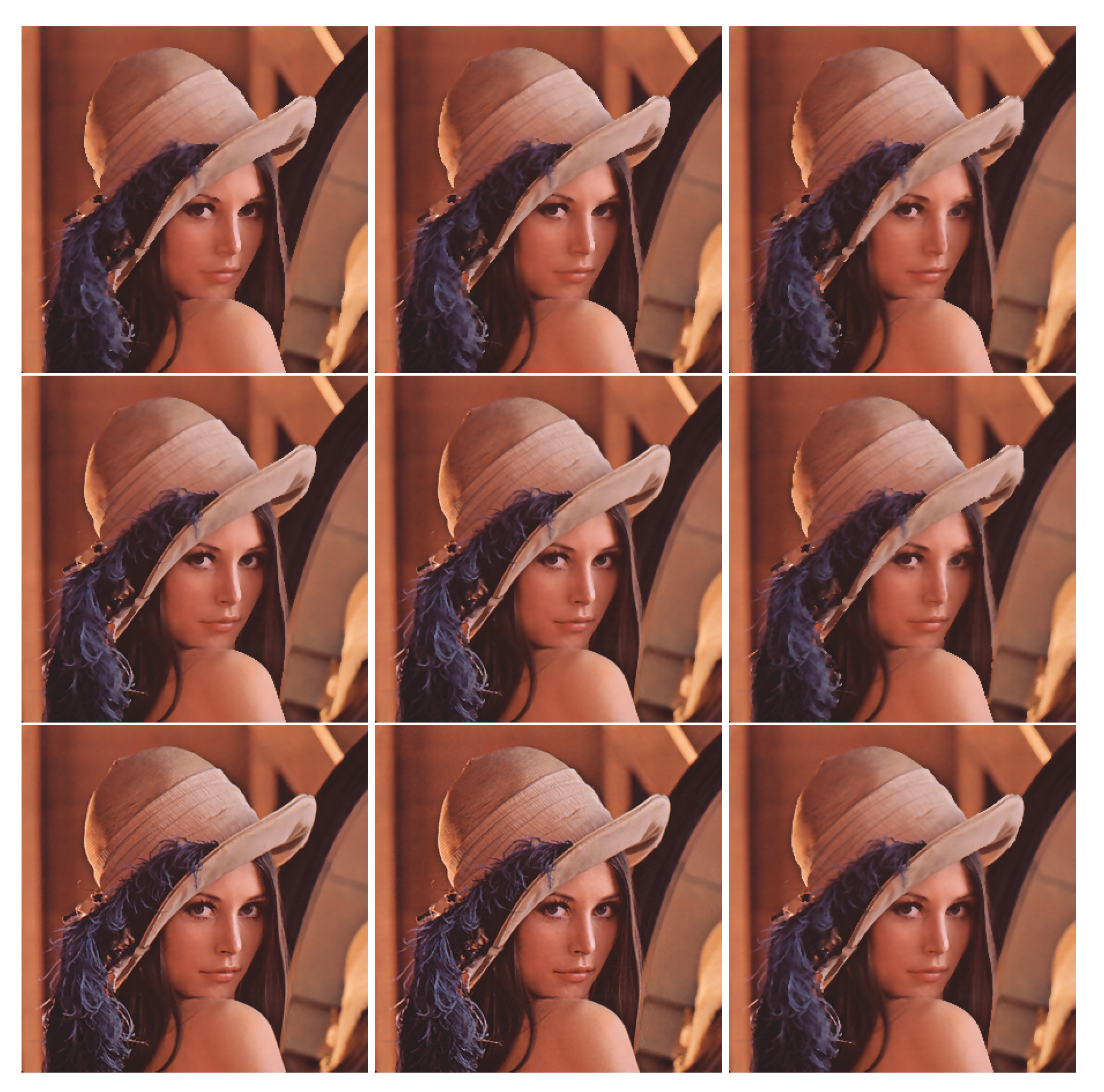
4. Some Illustrations of the Effects of Parameters p and $\lambda$

The process for calculating the p(x)-Laplacian on an image is that of the implementation in Algorithm 1. The effect parameters p and $\lambda$ of the model on an image are illustrated in Figure 2.

• In the case $0<p<1$, the pictures are partitioned into several homogeneous areas;
• In the case $1\le p\le 2$, when p approaches 2, there is a smoothing effect, whereas when p converges on 1 there is no smoothing effect;
• The increase in parameter $\lambda$ limits the effects of p.

Overall, when acting on the value of these parameters, several smoothing levels are reached which make the pictures striking or blurred.

Algorithm 1 Algorithm regularisation

x and j are positions in IM $IMF$ is the map result $IMT$ is a temporary map Compute gradient map G on image $IM$ Compute P map values on image $IM$ such as $P\left[x\right]:=1+\frac{1}{1+K{\left|G\left[x\right]\star IM\left[x\right]\right|}^2}$ $\epsilon$:= 0.01 $\lambda$:= user value in $[0;1]$ For all x in image $IM$    $IMF\left[x\right]$:=$IM\left[x\right]$    Do       $IMT\left[x\right]$:=$IMF\left[x\right]$       For j in neighbours of x            $IMF\left[x\right]:=IMF\left[x\right]+\frac{1}{P\left[j\right]\star G{\left[j\right]}^{P\left[j\right]}}$            $IMF\left[x\right]:=IMF\left[x\right]+\frac{\lambda }{2}\star \left|\right|IMF\left[j\right]-{IMT\left[j\right]\left|\right|}^2$    While $\left|IMF\right[x]-IMT[x\left]\right|>\epsilon$

4.1. Algorithmic Formulation of the Mathematical Model

4.1.1. Implementation Procedure

As in [4], an image is represented by a graph. In this structure, every vertex contains the coordinates of a pixel, and each edge indicates the difference between two pixels. The mathematical model in (26) is applied to the graph which must satisfy the existence and uniqueness requirements given in Section 3.1 into account.

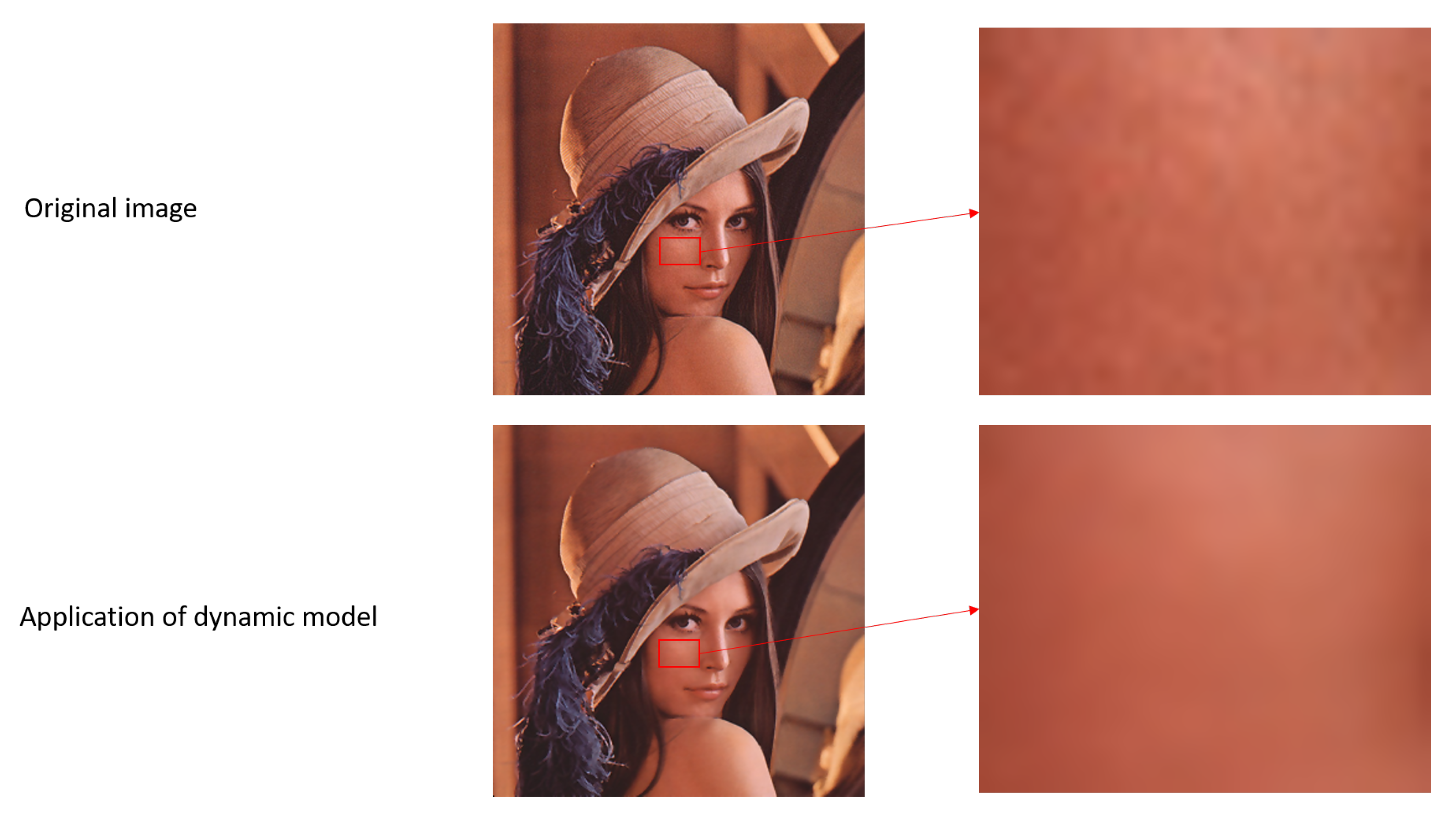
4.1.2. Towards an Adaptive Model

In the literature, the parameter p is often treated as static in the studies of this model. Otherwise, in our study, we propose to adapt parameter $\lambda$ in order to control the smoothing effects due to parameter p. The aim is to take account of the details in the image.

$\lambda$ model evaluation process to control the p effects: the parameters p and $\lambda$ play a crucial role in the dynamical smoothing process. Therefore, we calculate the difference in colour between a pixel and its neighbours in the following way. The gradient was chosen in accordance with the objective that had to be achieved.

Implementation of the parameter control process: In a preliminary step, we calculate the gradient of the image in order to detect prominent areas as well as noise. The idea is to vary the parameters in relation to the gradient in order to preserve details (areas of interest) and smooth out other areas. However, since the gradient is a local operator, it is sensitive to noise and also generates very large anomalous values that alter the process. For this reason, it is advisable to check the values obtained in each pixel in order to reduce the effect of the noise.

Efficient interval for the gradient: the three following types of pixels are focused on:

–

Noise-affected pixels;

–

Noise-unaffected pixels;

–

Outline pixels.

We would like to point out that the gradient values should be found by taking into account pixels (i.e., noise-affected and contour pixels which have the least effect on neighbouring pixels) that affect the process as little as possible. Thanks to these values, we will be able to create intervals that will allow us to select relevant values of the gradient. To do this, these intervals, defined by the interquartile deviation of the gradient distribution, are given by the statistical theory of data dispersion (see [17]) in the series according to the following formula

$$\left[Q_1-k(Q_3-Q_1),Q_3+k(Q_3-Q_1)\right]$$

(28)

where $Q_1$ and $Q_3$ are the first quartile and the third quartile, respectively. The positive constant k chosen as either 1.5 or 3 was discussed by Frigge et al. in [18].

These authors concluded for k that 1.5 is a suitable value for most situations. According to them, there are cases where 3 may be an appropriate compromise.

Thus, the following intervals were chosen:

$$I_{1.5}=\left[Q_1-1.5(Q_3-Q_1),Q_3+1.5(Q_3-Q_1)\right]$$

(29)

and

$$I_3=\left[Q_1-3(Q_3-Q_1),Q_3+3(Q_3-Q_1)\right]$$

(30)

For the interval $I_{1.5}$, the outer values correspond to major aberrant values (such as noise).

Study of the sturdiness of these criteria: After a series of tests on an image database, we found that the interval $I_{1.5}$ is noise-sensitive and allows one to consider areas to be smoothed. Algorithm 2 implements the process, and Figure 3 shows the effects of such a choice on two images.

Pixels that participate in the dynamic processing are shown in red. They will be submitted to variations in p and $\lambda$ depending on the gradient value. Pixels that will not be modified are shown in green. Their values are located in the highest gradient areas. The $\lambda$ values force the smoothing process to be neutralised. The adaptive model effects are shown in Figure 4.

We can see that the areas that are considered to be visually homogeneous (Lena’s skin texture, for example) are smoothed in order to further standardise the colours. On the contrary, the contours with a high gradient are preserved.

Algorithm 2 Algorithm regularisation with $\lambda$ dynamic

x and j are positions in IM $IMF$ is the map result $IMT$ is a temporary map Compute gradient map G on image $IM$ Compute P map values on image $IM$ such as $P\left[x\right]:=1+\frac{1}{1+K{\left|G\left[x\right]\star IM\left[x\right]\right|}^2}$ $\epsilon$:= 0.01 Compute quartile $Q_1,Q_2,Q_3,Q_4$ on the gradient norm Compute $\lambda$ map on image with quartile such as: $\lambda \left[x\right]=\left\{\begin{array}{cc}\hfill 1\hfill & \hfill ifgradientnormatxnotin{I}_{1.5}\hfill \\ \hfill 1-gradientnorm\hfill & \hfill else.\hfill \end{array}\right.$ For all x in image $IM$    $IMT\left[x\right]$:=$IM\left[x\right]$    Do       $IMF\left[x\right]$:=$IMT\left[x\right]$       For j in neighbours of x          $IMF\left[x\right]:=IMF\left[x\right]+\frac{1}{P\left[j\right]\star G{\left[j\right]}^{P\left[j\right]}}$          $IMF\left[x\right]:=IMF\left[x\right]+\frac{\lambda \left[x\right]}{2}\star \left|\right|IMF\left[j\right]-{IMT\left[j\right]\left|\right|}^2$    While $\left|IMF\right[x]-IMT[x\left]\right|>\epsilon$

5. Results and Discussion

Presentation of the database and discussion of execution times and complexity

We used two images to illustrate the treatments:

–

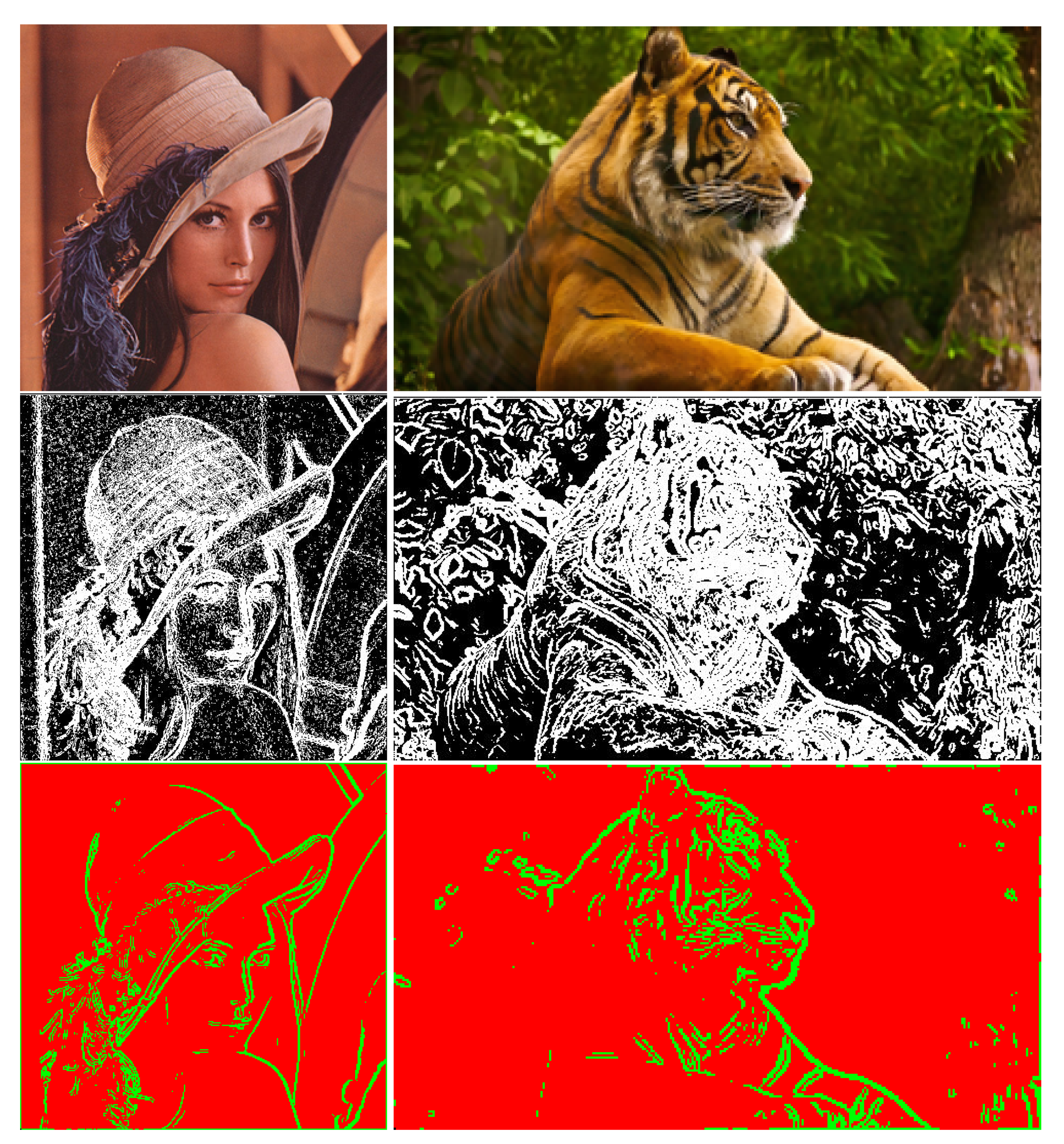
Lena image, which is widely used in image processing;

–

Tiger image, because it contains the most significant data in image processing. The tiger is present within the focal depth, while the rest of the scene, which is less important, should be homogenised.

The execution of the programme mainly depends on the smoothing factor and the number of pixels to be smoothed. The higher the smoothing factor, the more a pixel must be modified. Processing continues until every pixel in the image is stabilised. The complexity is in $\mathcal{O}\left(kN\right)$, where N is the number of pixels in an image and k is a constant representing the disorder in the original image. By increasing the value of $\lambda$ in detailed areas, the proposed model reduces the processing time. Figure 5 shows the results of the adaptive model on noise.

We used the adaptive model on 100 images of the Berkeley database set [19]. This database contains colour photographs of various scenes. The results of these studies are presented in the following sections.

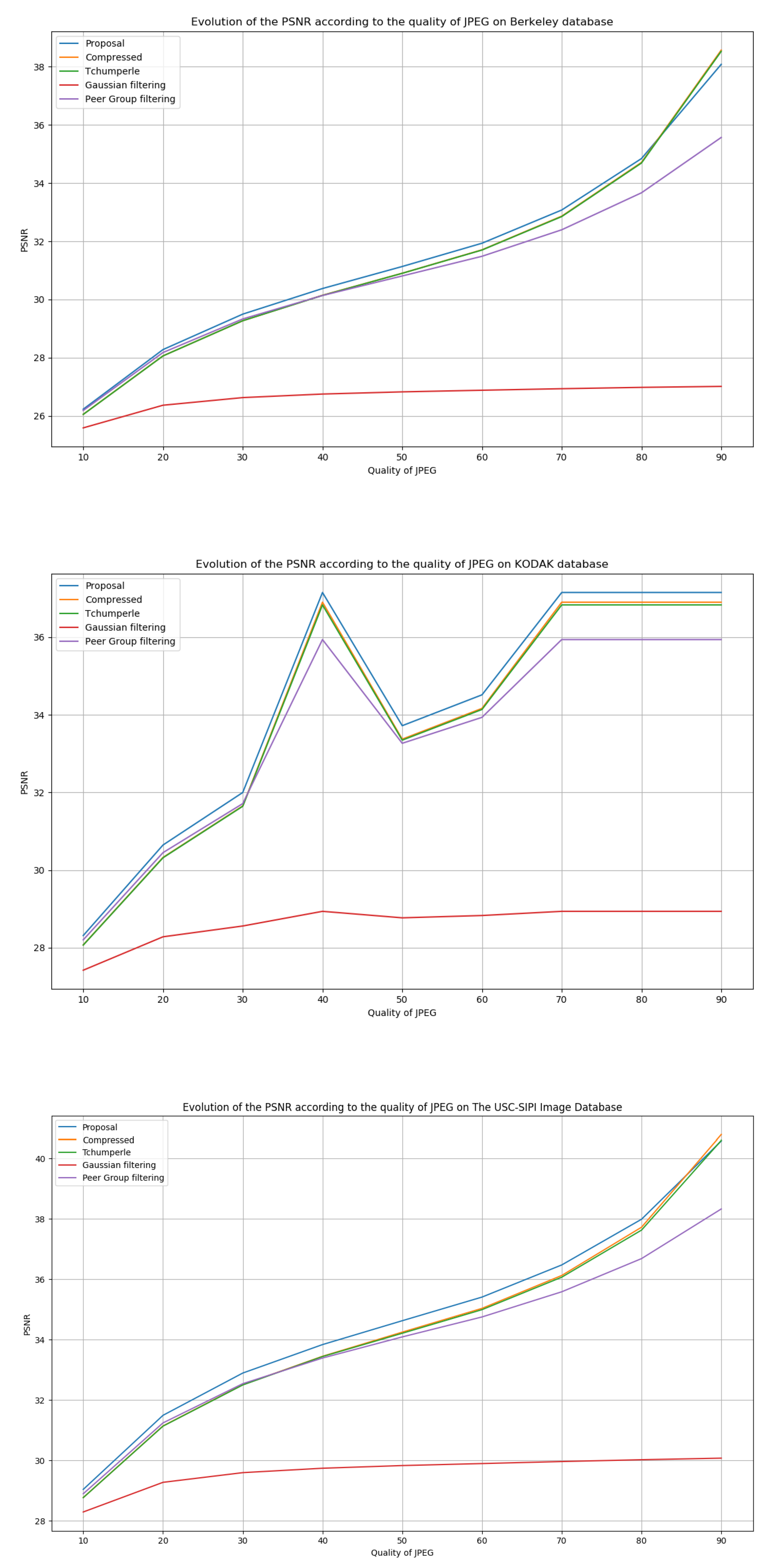
5.1. Results with the Peak Signal-to-Noise Ratio (PSNR)

We evaluated the quality of the filtering using the peak signal-to-noise ratio (PSNR) in a first work. This parameter is used to calculate the presence of noise in an image. Its formulation is described in (31):

$$PSNR=10\times lo{g}_{10}\left(SNR\right)$$

(31)

$$\begin{array}{cc}\hfill SNR& \hfill =\frac{signal}{noise}\hfill \\ & \hfill =\frac{I_{original}}{I_{original}-I_{noisy}}\hfill \\ & \hfill =\frac{{\displaystyle \sum _x}{\displaystyle \sum _y}{I}_{original}^2(x,y)}{{\displaystyle \sum _x}{\displaystyle \sum _y}{\left(I_{original}(x,y)-I_{noisy}(x,y)\right)}^2}.\hfill \end{array}$$

(32)

In our study, there are no noiseless images, and so we go back to the formula in (33) to evaluate the quality of the images from the dynamic processing.

$$SNR=\frac{I_{filtered}}{I_{filtered}-I_{original}}$$

(33)

The values obtained can be compared with the reference values in

Table 1. Relationship between PSNR and image quality.

PSNR	Image Quality
30	Excellent
24.99	Good
20	Reasonable
15.05	Very noisy
10	Unreadable

. The values obtained on Lena’s image after varying p and $\lambda$ are shown in

Table 2. Result of using PSNR on the Lena image (Figure 2) by varying p and $\lambda$.

PSNR	p = 0.01	p = 1.00	p = 2.00
$\lambda$ = 0.01	28.98	29.61	26.57
$\lambda$ = 0.10	33.80	36.46	27.49
$\lambda$ = 1.00	41.47	45.81	32.83

. These values can be compared with the reference values given in Table 1.

The Lena image with the adaptive model provides a PSNR = 27.66, while the tiger image gives a PSNR = 24.31. In order to validate the proposed filter, we chose to use the adaptive model on 100 images extracted from the Berkeley database [19] (see Figure 6), 14 images extracted from the USC-SIPI Image Database [20] (see Figure 7), and 24 images extracted from Kodak Lossless True Color Image Suite [21] (see Figure 8). Images from these databases are widely known and show different scenes with contrasts.

From the Berkeley database,

Table 3. DSSIM parameter values obtained on images of Figure 9. The Sobel columns give the number of points designating the contours as well as the noise.

Image	PSNR	DSSIM	Sobel on Original	Sobel on Adaptive
a	36.247566	0.002315	15,193	10,841
b	36.034393	0.002149	19,850	17,310
c	26.577696	0.002279	55,113	54,321
d	26.364088	0.003355	55,454	54,567

and

Table 4. Statistical results on the PSNR obtained with the adaptive model on the Berkeley database.

	Average	Min	Max	Standard Deviation
PSNR	31.13	26.36	36.24	2.19

show the DSSIM and PSNR results obtained, and Figure 9 shows two images that obtained the best PSNR following the application of the adaptive model as well as the two images with the worst PSNR.

The values presented in Table 4 are quite homogeneous, as can be seen from the standard deviation, which remains at 2.19, and the average PSNR, which remains at 31.13. This last value represents a good image quality according to this parameter. With regard to the sample used, 26.36 corresponds to a minimum PSNR. It places the worst case towards a good result. Otherwise, for an image quality considered excellent, 36.24 is the best PSNR obtained by the adaptive model.

5.2. Results with the Structural Dissimilarity Measure (DSSIM)

In the first stage, we use structural dissimilarity DSSIM [22] to assess the quality of filtering, and

Table 5. The result of using the DSSIM parameter on the Lena image (Figure 2) by varying p and $\lambda$.

DSSIM	p = 0.01	p = 1.00	p = 2.00
$\lambda$ = 0.01	0.07	0.06	0.11
$\lambda$ = 0.10	0.02	0.01	0.09
$\lambda$ = 1.00	0.004	0.001	0.02

shows the results obtained. This measure was developed to evaluate the visual quality of a compressed image with respect to the original image. It uses the SSIM parameter (structural similarity) to measure the similarity of structure between the two images. Its formula is given by (34):

$$DSSIM(x,y)=\frac{1-SSIM(x,y)}{2}$$

(34)

with

$$SSIM(x,y)=\frac{(2{\mu }_x{\mu }_y+c_1)(2{\sigma }_x{\sigma }_y+c_2)(2co{v}_{xy}+c_3)}{({\mu }_x^2+{\mu }_y^2+c_1)({\sigma }_x^2+{\sigma }_y^2+c_2)({\sigma }_x{\sigma }_y+c_3)}$$

where ${\mu }_x$ and ${\mu }_y$ are averages in the x and y direction, and ${\sigma }_x^2$ and ${\sigma }_y^2$ are the variances of x and y, respectively. $c_1,c_2,c_3$ are parameters needed to stabilise the division.

In order to simulate the images from the network, we compressed all images in the dataset. For this study, we chose to use JPEG compression. The images available in the database were compressed in JPEG format with several compression ratios ranging from 10% to 90% quality. We have already shown the impact of dynamic $\lambda$ with respect to static $\lambda$.

Table 6. Illustrations of DSSIM results obtained from 100 images extracted from the Berkeley database. This study was carried out according to the compression ratio in order to simulate degradation, and different values taken for $\lambda$ were compared to the method used for dynamic $\lambda$ (bold values represent the best results).

Compression/$\mathit{\lambda }$	0.1	0.5	1.0	Proposal Model
10%	0.124749391	0.124685624	0.126527000	0.126313566
20%	0.073399066	0.067223833	0.067583050	0.067538158
30%	0.0590243333	0.0504784583	0.050169525	0.050176050
40%	0.052676424	0.0429842166	0.042350825	0.042386891
50%	0.048671533	0.0382977916	0.0374521999	0.0374951749
60%	0.045554683	0.0346366000	0.0336435749	0.033697841
70%	0.0423388583	0.030723008	0.02957985	0.0296397499
80%	0.039299400	0.0268465583	0.0255539583	0.0256166749
90%	0.036822691	0.023159216	0.0215449250	0.0216251499

summarises this study.

The algorithmic process gives the best values in the dynamic $\lambda$ case and where $\lambda$ is 1.0. In terms of the DSSIM criterion, these two cases give better results. However, the $\lambda$ value of 1.0 leads to too much smoothing over the whole image, as shown in Figure 10.

In a second step, we compare one side of the original image with the compressed image and the other side with the compressed image after applying our filtering. We used other filtering algorithms in the evaluation process. The method of D. Tschumperle [23] was used, which consists of regularising an image by an anisotropic smoothing process based on PDEs. This model requires parameterisation for its implementation, so we used standard values given in the literature. Gaussian filtering was used, which consists of applying a Gaussian filter to the rows and then to the columns of the image. Peer group filtering was used, which allows an image to be smoothed by replacing a pixel with the weighted sum of its closest neighbours in terms of colour distance. The purpose was to observe whether our proposal leads to improvements in terms of visual rendering, especially in the case of high losses. The results obtained with PSNR and DSSIM are shown in Figure 11 and Figure 12 (for PSNR, a higher value is better, whilst for DSSIM, a lower value is better).

In Figure 11 and Figure 12, the curve representing the compressed image expresses the relevance of the models. In fact, in the case of PSNR, this relevance is provided by a model that gives results above the compressed image and, up to the case of DSSIM, by a model that gives results below the compressed image. However, the use of Gaussian filtering does not satisfy these conditions. In the worst case, the others are generally confused by the compressed image. Finally, we observed, with the help of

Table 7. Illustration of the mean values and standard deviations on DSSIM and PSNR criteria obtained after image processing by our proposed model on the Berkeley (120 images), Kodak (24 images), and USC-SIPI (13 images) databases.

	Berkeley Databases		KODAK Databases		USC-SIPI Databases
	DSSIM	PSNR	DSSIM	PSNR	DSSIM	PSNR
10%	0.13 (0.02)	26.23 (2.07)	0.1 (0.01)	28.31 (2.3)	0.09 (0.01)	30.07 (2.63)
20%	0.07 (0.013)	28.28 (2.19)	0.05 (0.009)	30.64 (2.44)	0.05 (0.009)	32.7 (2.97)
30%	0.05 (0.01)	29.49 (2.23)	0.03 (0.007)	32 (2.45)	0.04 (0.008)	34.14 (3.15)
40%	0.04 (0.01)	30.37 (2.22)	0.03 (0.005)	32.9 (2.43)	0.03 (0.007)	35 (3.19)
50%	0.04 (0.009)	31.13 (2.19)	0.02 (0.005)	33.72 (2.39)	0.03 (0.007)	35.6 (3.18)
60%	0.03 (0.009)	31.93 (2.14)	0.02 (0.004)	34.52 (2.33)	0.02 (0.007)	36.36 (3.16)
70%	0.03 (0.008)	33.07 (2.03)	0.02 (0.004)	35.58 (2.22)	0.02 (0.007)	37.23 (3.08)
80%	0.03 (0.008)	34.81 (1.84)	0.01 (0.003)	37.15 (2)	0.02 (0.007)	38.41 (2.9)
90%	0.02 (0.008)	38.07 (1.41)	0.01 (0.003)	39.88 (1.5)	0.02 (0.007)	40.58 (2.33)

, using the standard deviation, the stability of the results on all the databases used in this work.

Table 8. Presentation of the average execution times of the adaptive p(x)-Laplacian model on the image databases used in the experiment.

	Average Time in Seconds
	Berkeley Databases	KODAK Databases	USC-SIPI Databases
10%	601.80	854.96	505.35
20%	464.79	966.35	423.26
30%	517.82	928.12	601.09
40%	471.24	911.41	505.01
50%	538.31	741.18	367.47
60%	540.24	794.21	428.84
70%	527.51	657.88	520.70
80%	468.22	866.27	553.07
90%	437.38	758.04	603.88

shows the average execution times achieved by our model on the image databases used. The algorithm still needs to be optimized to reduce the time required to process an image. The average processing time observed is approximately 10 min per image.

When using the PSNR parameter, the visual rendering is improved for compression with a quality between 10% and 70%. The use of the DSSIM parameter shows that, for a quality of between 10% and 30%, the proposed model improves. In any case, for compression with high information loss, our proposal gives better PSNR and DSSIM values than the just compressed image. As soon as the compression becomes low, we see that it is no longer necessary to use our proposal, since it provides values that are lower than those given by the compressed image.

The work focuses on the proposal of an adaptive control operator for the smoothing strength of the p(x)-Laplacian method. Tests were carried out on the three following image databases: Berkeley, USC-SIPI, and KODAK. We degraded the images of these three databases by applying compression levels with losses. The results in Figure 11 and Figure 12 show a higher efficiency of the p(x)-Laplacian method with our adaptive controller compared to other smoothing methods in the literature with respect to the PSNR and DSSIM evaluation operators. We showed that the p(x)-Laplacian operator with our control operator produces better results than the p(x)-Laplacian with a static $\lambda$. Our method produces a $\lambda$ value for each point of the image adapted to the situation, as shown in the examples in Table 6 with respect to the DSSIM evaluation criterion. Finally, we compared the p(x)-Laplacian with our control operator to other smoothing models in the literature, still based on the same principle of degradation of all images in the datasets. Our proposal gives better results, although for the KODAK image database, we still have roughly equivalent results in terms of the PSNR evaluation criterion.

The contribution of an adaptive controller of the $\lambda$ parameter of the p(x)-Laplacian operator has not yet been studied in the literature. Our contribution, which aims to control its smoothing strength according to the locations of an image, shows an improvement in the results obtained using this operator. In a final study, we used two noise generation methods from the literature, again based on the image databases Berkeley, KODAK, and USC-SIPI. These methods consist of creating random additive noise to the images based on a probability law for the distribution, such as the Gaussian distribution or the Poisson distribution. The results of applying these methods and then correcting them using the methods presented in this work are shown in

Table 9. Results of the evaluation of the application of smoothing methods on the Berkeley, KODAK, USC-SIPI noisy image databases using the Gaussian-distributed additive noise method.

		Gaussian-Distributed Additive Noise
Images	Filtering Method	DSSIM (sd)	PSNR (sd)
Berkeley	Proposal (2)	0.019 (0.007)	42.495 (1.385)
	Tchumperle (1)	0.016 (0.007)	55.810 (2.214)
	Gaussian filtering (4)	0.069 (0.021)	27.028 (2.571)
	Peer group filtering (3)	0.020 (0.007)	37.556 (2.840)
KODAK	Proposal (2)	0.006 (0.003)	44.052 (1.085)
	Tchumperle (1)	0.005 (0.003)	54.110 (2.205)
	Gaussian filtering (4)	0.045 (0.020)	29.020 (2.963)
	peer Group filtering (3)	0.007 (0.003)	40.094 (2.988)
USC-SIPI	Proposal (2)	0.014 (0.007)	44.559 (1.733)
	Tchumperle (1)	0.013 (0.007)	53.738 (3.184)
	Gaussian filtering (4)	0.035 (0.019)	30.972 (3.031)
	Peer group filtering (3)	0.015 (0.007)	42.382 (3.374)

and

Table 10. Results of the evaluation of the application of smoothing methods on the Berkeley, KODAK, USC-SIPI noisy image databases using the Poisson-distributed noise generated method.

		Poisson-Distributed Noise
Images	Filtering Method	DSSIM (sd)	PSNR (sd)
Berkeley	Proposal (2)	0.019 (0.007)	42.338 (1.364)
	Tchumperle (1)	0.016 (0.007)	51.841 (0.957)
	Gaussian filtering (4)	0.069 (0.021)	27.027 (2.571)
	Peer group filtering (3)	0.020 (0.007)	37.488 (2.792)
KODAK	Proposal (2)	0.007 (0.003)	43.908 (1.079)
	Tchumperle (1)	0.005 (0.003)	51.311 (1.205)
	Gaussian filtering (4)	0.045 (0.020)	29.017 (2.963)
	Peer group filtering (3)	0.007 (0.003)	39.948 (2.914)
USC-SIPI	Proposal (2)	0.014 (0.007)	44.434 (1.716)
	Tchumperle (1)	0.013 (0.007)	51.266 (1.857)
	Gaussian filtering (4)	0.036 (0.019)	30.971 (3.030)
	Peer group filtering (3)	0.015 (0.007)	42.167 (3.261)

. Overall, we can see that the proposed method ranks second only to the Tchumperle method.

6. Conclusions and Prospects

In the field of image enhancement, smoothing methods are used to correct singularities. Among these methods, we are interested in the p(x)-Laplacian. It is generally used in the literature with a fixed control parameter. This choice does not allow for finer processing over the entire image. We proposed to apply this nonlinear regularisation operator, which we have made adaptive, in order to emphasise important visual information. We therefore proposed an adaptive control criterion that controls smoothing as a function of the image gradient, which we exploited using statistics. In order to evaluate this new model, we used the PSNR and DSSIM parameters. The former indicates a good reconstruction quality when its value is above 24 dB, and the latter assesses the quality of the filtering. From our test database, the results obtained put the average PSNR at 24.80 dB, with the worst result around a reasonable reconstruction. According to the DSSIM parameter, the quality of the image improved, provided that it had undergone many degradations, such as lossy compression.

References

1. Bougleux, S.; Elmoataz, A.; Melkemi, M. Local and nonlocal discrete regularisation on weighted graphs for image and mesh processing. Int. J. Comput. Vis. 2009, 84, 220–236. [Google Scholar] [CrossRef]
2. Chambrolle, A.; Lions, P. Image recovery via total variation minimization and related problems. Numer. Math. 1997, 76, 167–188. [Google Scholar] [CrossRef]
3. Rudin, L.; Osher, S.; Fatemi, E. Nonlinear total variation based noise removal algorithm. Phys. D 1992, 60, 259–268. [Google Scholar] [CrossRef]
4. Chen, Y.; Levine, S.; Rao, M. Variable exponent, linear growth functionals in image restoration. SIAM J. Appl. Math. 2006, 66, 1383–1406. [Google Scholar] [CrossRef]
5. Coren, S.; Girgus, J.S. Principles of perceptual organization and spatial distortion: The gestalt illusions. J. Exp. Psychol. Hum. Percept. Perform. 1980, 6, 404–412. [Google Scholar] [CrossRef] [PubMed]
6. Ricard, J.; Baskurt, A.; Idrissi, K.; Lavoue, G. Object of interest-based visual navigation, retrieval, and semantic content identification system. Comput. Vis. Image Underst. 2004, 94, 271–294. [Google Scholar]
7. Bollt, E.M.; Chartrand, R.; Esedoglu, S.; Schultz, P.; Vixie, K.R. Graduated adaptive image denoting local compromise between total variation and isotropic diffusion. Adv. Comput. Math. 2009, 61–85. [Google Scholar] [CrossRef]
8. Harjuletho, P.; Hästö, P.; Latvala, V. Minimizers of the variable exponents, nonuniformly convex Dirichlet energy. J. Math. Pures Appl. 2008, 89, 174–197. [Google Scholar] [CrossRef]
9. Musielak, J. Orlicz Spaces and Modular Spaces; Springer: Berlin/Heidelberg, Germany, 2010. [Google Scholar]
10. Diening, L.; Harjulehto, P.; Hasta, P.; Ruzicka, M. Lebesgue and Sobolev Spaces with Variable Exponents; Springer: Berlin/Heidelberg, Germany, 2017. [Google Scholar]
11. Kovacik, O.; Rakosnik, J. On spaces Lp(x) and Wk,p(x). Czechoslov. Math. J. 1991, 41, 592–618. [Google Scholar]
12. Brezis, H. Analyse Fonctionnelle Théorie et Applications Masson et Cie 1983. Available online: https://cir.nii.ac.jp/crid/1571135649569314304 (accessed on 10 February 2023).
13. Elmoataz, A.; Olivier, L.; Bougleux, S. Nonlocal discrete regularisation on weigthed graphs: A framework for image and manifold processing. IEEE Trans. Image Process. 2008, 17, 1047–1060. [Google Scholar] [CrossRef] [PubMed]
14. Elmoataz, A.; Desquesnes, X.; Lezoray, O. Non-Local Morphological PDEs and p-Laplacian Equation on Graphs With Applications in Image Processing and Machine Learning. IEEE J. Sel. Top. Signal Process. 2012, 6, 764–779. [Google Scholar] [CrossRef]
15. Ta, V.T.; Elmoataz, A.; Lezoraty, O. Nonlocal PDEs-based morphology on weighted graphs for image and data processing. IEEE Trans. Image Process. 2011, 20, 1504–1516. [Google Scholar] [PubMed]
16. Zhou, D.; Schölkopf, B. Regularization on Discrete Spaces. In Proceedings of the Pattern Recognition; Kropatsch, W.G., Sablatnig, R., Hanbury, A., Eds.; Springer: Berlin/Heidelberg, Germany, 2005; pp. 361–368. [Google Scholar]
17. Albarello, L.; Bourgeois, E.; Guyot, J.L. Statistique Descriptive: Un Outil Pour Les Praticiens Chercheurs; De Boeck Supérieur: Louvain-la-Neuve, Belgium, 2010. [Google Scholar]
18. Frigge, M.; Hoaglin, D.C.; Iglewicz, B. Some implementations of the boxplot. Am. Stat. 1989, 43, 50–54. [Google Scholar]
19. Martin, D.; Fowlkes, C.; Ta, D.; Malik, J. A Database of Human Segmented Natural Images and its Application to Evaluating Segmentation Algorithms and Measuring Ecological Statistics. In Proceedings of the Eighth IEEE International Conference on Computer Vision, ICCV 2001, Vancouver, BC, Canada, 7–14 July 2001; Volume 2, pp. 416–423. [Google Scholar]
20. Weber, A.G. The USC-SIPI Image Database Version 5. USC-SIPI Report 1997, 315. Available online: https://cir.nii.ac.jp/crid/1573950399791107200 (accessed on 27 January 2023).
21. Franzen, R. Kodak Lossless True Color Image Suite. 1999, 4. Available online: http://r0k.us/graphics/kodak (accessed on 27 January 2023).
22. Wang, Z.; Bovik, A.C.; Sheikh, H.R.; Simoncelli, E.P. Image quality assessment: From error visibility to structural similarity. IEEE Trans. Image Process. 2004, 13, 600–612. [Google Scholar] [CrossRef] [PubMed]
23. Tschumperlé, D. Fast anisotropic smoothing of multi-valued images using curvature-preserving PDE’s. Int. J. Comput. Vis. 2006, 68, 65–82. [Google Scholar] [CrossRef]
Figure 1. Comparison between a degraded and a non-degraded image. Above: BMP, 2160 × 3840, 23.7 MB; below: an image which has been compressed, 2160 × 3840, 4.8 MB.
Applsci 13 11600 g001
Figure 2. Effects of parameters p and λ on the Lena image. From left to right, parameter p increases to values { 0.01 ; 1.00 ; 2.00 } . From top to bottom, the lambda increases by taking values { 0.01 ; 0.10 ; 1.00 } .
Applsci 13 11600 g002
Figure 3. Illustration of the interval I 1.5 effects. The (first line) shows the original images, the (second line) shows the result of the edge and noise detection, and the last line shows the result of the proposed classification. More specifically, the pixels that have a gradient value in the interval are shown in red and the pixels with a value outside of this interval are shown in green.
Applsci 13 11600 g003
Figure 4. Illustration of the adaptive model effects on the Lena image.
Applsci 13 11600 g004
Figure 5. Illustration the effects of the adaptive model. From top to bottom, the original images, the result of applying the Sobel filter, then the result of applying the adaptive algorithm, and finally the result of applying the Sobel filter. The application of the proposed adaptive method reduces the number of noise and contour points for the Lena image from 21,571 pixels to 19,552 pixels (a reduction of 9.35%) and for the Tiger image from 15,600 to 14,374 (a reduction of 7.86%).
Applsci 13 11600 g005
Figure 6. Illustration of the images contained in the Berkeley database.
Applsci 13 11600 g006
Figure 7. Illustration of the images contained in the USC-SIPI databases.
Applsci 13 11600 g007
Figure 8. Illustration of the images contained in the KODAK database.
Applsci 13 11600 g008
Figure 9. Illustrations of the results obtained by testing 100 images extracted from the Berkeley database with an alteration (a degraded aspect due to, for instance, bad capture or compression) with a ratio of almost 50%. From top to bottom (ad), we note the two best results and the two worst results obtained using the PSNR and DSSIM parameters. From left to right, the original degraded image followed by the result of the application of the Sobel filter, then the result of the application of the adaptive algorithm on the degraded image, and finally, the result of the Sobel filter. In all cases, there is a decreasing number of pixels with a high gradient.
Applsci 13 11600 g009
Figure 10. Illustration of the effects of the use of static λ and dynamic λ on the Lena image. (Left side) λ = 1.0 ; (Right side) λ is dynamic.
Applsci 13 11600 g010
Figure 11. Results on the evolution of the PSNR according to the quality of compression.
Applsci 13 11600 g011
Figure 12. Results on the evolution of the DSSIM according to the quality of the compression.
Applsci 13 11600 g012