Tire Defect Detection via 3D Laser Scanning Technology

Abstract

Tire defect detection, as an important application of automatic inspection techniques in the industrial field, remains a challenging task because of the diversity and complexity of defect types. Existing research mainly relies on X-ray images for the inspection of defects with clear characteristics. However, in actual production lines, the major threat to tire products comes from defects of low visual quality and ambiguous shape structures. Among them, bubbles, composing a major type of bulge-like defects, commonly exist yet are intrinsically difficult to detect in the manufacturing process. In this paper, we focused on the detection of more challenging defect types with low visibility on tire products. Unlike existing approaches, our method used laser scanning technology to establish a new three-dimensional (3D) dataset containing tire surface scans, which leads to a new detection framework for tire defects based on 3D point cloud analysis. Our method combined a novel 3D rendering strategy with the learning capacity of two-dimensional (2D) detection models. First, we extracted accurate depth distribution from raw point cloud data and converted it into a rendered 2D feature map to capture pixel-wise information about local surface orientation. Then, we applied a transformer-based detection pipeline to the rendered 2D images. Our method marks the first work on tire defect detection using 3D data and can effectively detect challenging defect types in X-ray-based methods. Extensive experimental results demonstrate that our method outperforms state-of-the-art approaches on 3D datasets in terms of detecting tire bubble defects according to six evaluation metrics. Specifically, our method achieved 35.6, 40.9, and 69.1 mAP on three proposed datasets, outperforming others based on bounding boxes or query vectors.

1. Introduction

Automatic detection technology plays an important role in many fields of industrial quality inspection, such as those for steel [1], solar wafers [2], airplanes [3], and fabrics [4,5,6]. Compared with human inspection, automatic defect detection has high accuracy and efficiency, which significantly lowers the risk of human intervention in hazardous environments. With the fast advancements in computer vision in the past two decades, an increasing number of vision-based quality inspection technologies has been applied in many real-world applications. Thanks to the learning capacity and generalization ability of advanced detection methods, such as convolutional neural networks (CNNs [7] and transformers [8,9]), training models with an insufficient number of training data in various scenarios of the industrial field have become possible.

With the demand for intelligent manufacturing, defect detection techniques have become a rising topic in the tire industry for quality inspection. Because of external factors of the manufacturing process and the mechanical environment, tire products inevitably suffer from various types of defects. Among these defects, bulges are a major concern in actual production lines, especially for tires used in engineering vehicles. The causes of this type of defect can be summarized into two types: (1) Rubber particles or other impurities are mixed between the interior layers of the tire, leading to a clear bulge on the tire surface (impurity bulges). (2) External air or high-temperature chemical components are not fully eliminated during production (bubbles). With the advances in mechanical devices and manufacturing techniques, the formation of impurity bulges has been significantly reduced in tire industries. However, bubble defects are still a major threat to the quality and reliability of tire products, which are dangerous to driving conditions. Existing research on tire defect detection treats different bulges as a general type of defect and mainly focuses on impurity bulges that have distinctive features. However, bubble defects present a visual quality very similar to those of surrounding areas, making them extremely difficult to detect in the manufacturing process.

Because of the intrinsic limitations of detecting defect types with very low visibility, the inspection of bubble defects on tire surfaces remains a challenging task in both academic and industrial fields. A common way to detect bubbles is via human–eye inspection in real production lines. Such a process requires experienced workers with the help of strong light sources to reveal possible irregular surface areas, which is time-consuming and has low accuracy (see Figure 1a). Meanwhile, other typical types of tire defects, such as exposed cords or cracking, are normally detected using X-ray inspection techniques [10,11,12], where radiographic images are captured to detect defects with clear sharp edges or color differences. Unfortunately, considering the extremely low visual quality of bubble defects, X-ray scans are insensitive to this type of defect, as shown in Figure 1. Another solution is the use of laser speckles techniques, but this method is not very common in industrial defect detection. During processing, an inspected tire should be placed in a vacuum space where the inner air pressure could extend the size of bubble defects. By comparing speckle patterns before and after processing, locating smaller bulges on tire surfaces is easier. However, this solution requires complicated procedures and is inefficient for real-time inspection.

Considering the difficulty and inefficiency of detecting bubble defects in tire defect detection, we aimed to search for a more suitable solution that can capture these defects’ characteristics for efficient inspection. Despite their different natures, bulge-like defects can be defined as irregular areas on the relatively flat surface of a tire product, presenting certain features in terms of depth distribution. Therefore, we extracted three-dimensional (3D) surface data for the detection of bubble defects and established a new dataset of scanned tire surfaces using laser scanners, which were then presented as 3D point clouds. Thanks to the development of 3D acquisition techniques, today’s scanners can provide accurate results with less than 0.1 mm of scanning error, providing accurate data for detecting smaller characteristics. We show in Figure 1d that very small bulges can be reflected as points arranged in a curved scanning line even though they are hardly visible in the two-dimensional (2D) domain. By analyzing the point distribution in the 3D domain, such defects are much easier to detect at very small scales.

We propose a new tire defect detection pipeline unlike previous methods by combining both 3D and 2D information for analyzing and detecting bulge-like tire defects. Because of the irregularity and sparse nature of 3D point cloud data, the raw scanned surface may contain undesired scanning noise and regular textures on the tire surface. Therefore, locating accurate positions of the target defects from the raw 3D scans is intrinsically difficult (see Figure 1d). Moreover, we propose the combination of the captured 3D information and 2D detection pipelines to take advantage of the powerful learning capacity of existing detection models. Our method consists of two main stages. In the first stage, we extract 3D information from the raw point cloud data and estimate the surface curvature of each point in its local region using a normal-based rendering strategy. A rendered 2D feature map (see Figure 1e) is obtained for the subsequent detection model, which contains pixel-wise surface orientation for detecting irregular bulges on the scanned surface. Second, given the obtained feature map, we design a transformer-based detection network to predict possible areas of the target defects. The qualitative and quantitative results demonstrate that our method outperforms existing tire-defect-detection methods in terms of detection accuracy. Our contribution can be summarized as follows:

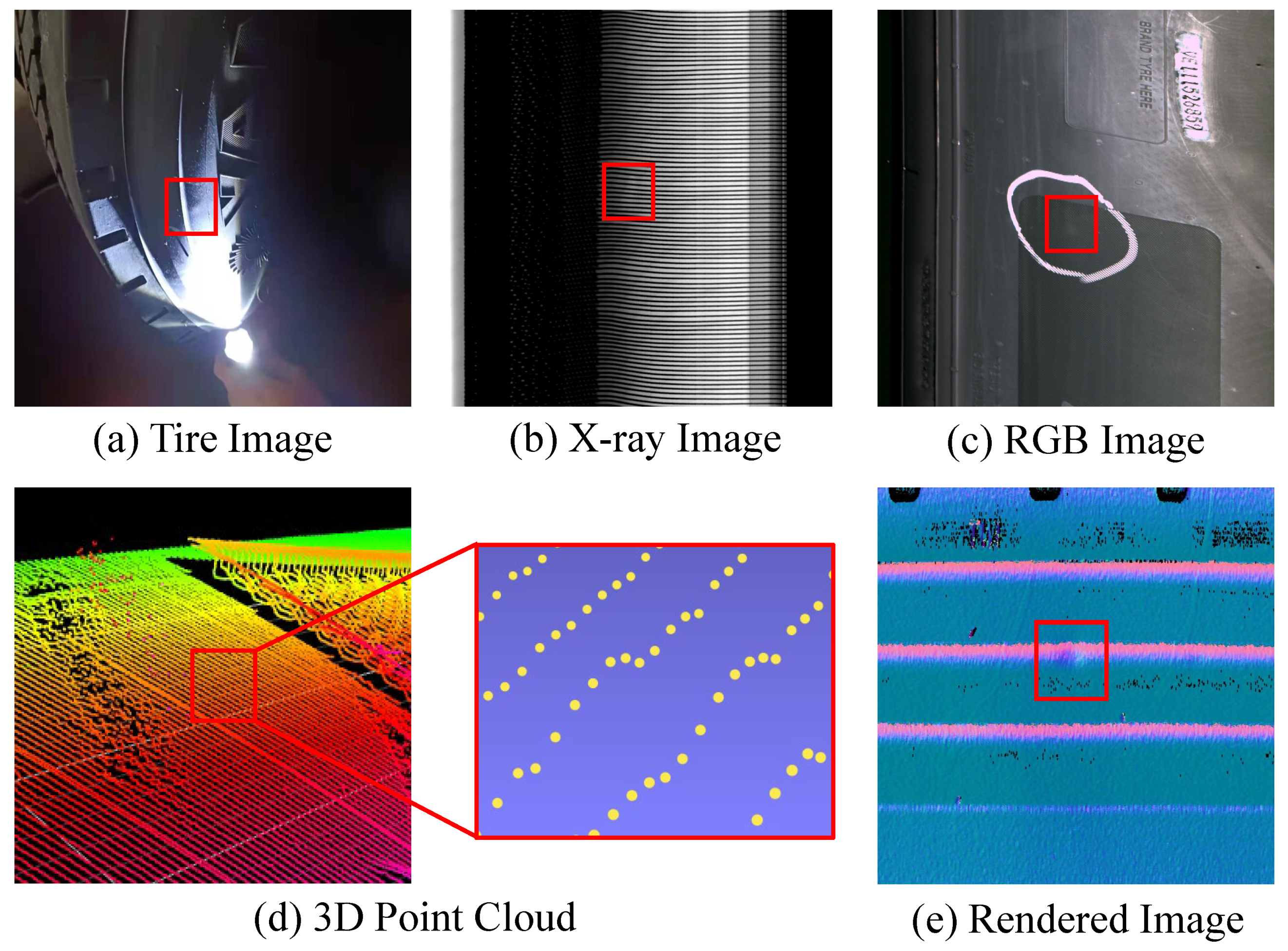
• Our method is the first work focusing on the detection of low-visibility tire defects and establishes a new 3D dataset consisting of scanned tire surfaces from laser scanners.
• We propose a new detection pipeline for tire defects by combining 3D surface data and a 2D detection model to effectively detect challenging tire defects.
• We design a normal-based rendering strategy to extract surface orientation from scanned raw point clouds, which provides effective 2D depth information for the subsequent detection process.
• We apply a novel transformer-based detection model for detecting accurate areas of target defects.

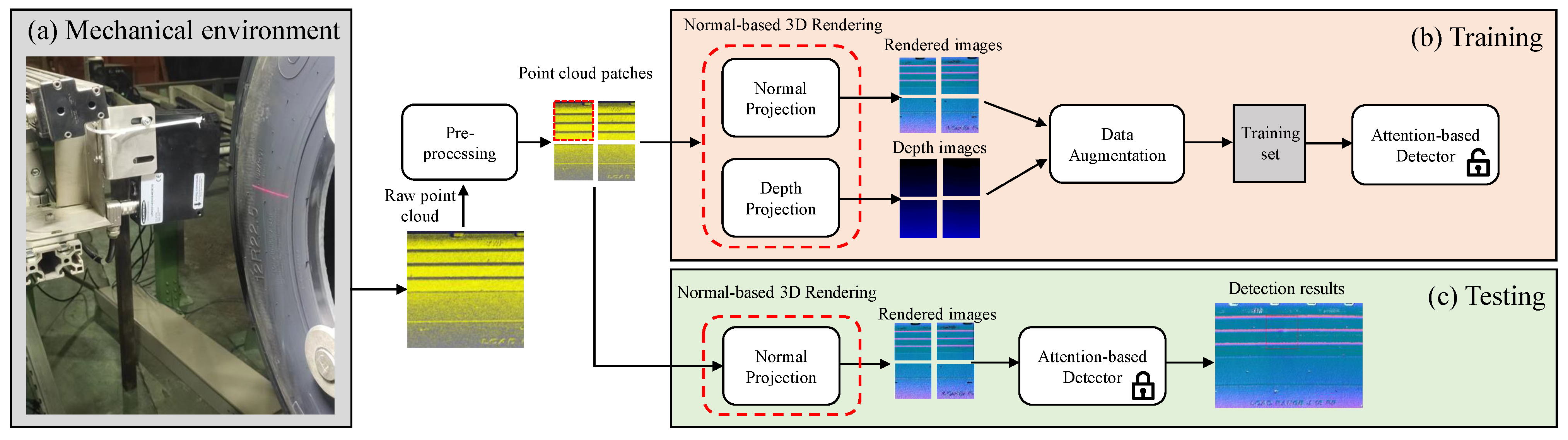
2. Materials and Methods

The overall pipeline of our proposed tire-defect-detection method is shown in Figure 2. First, a preprocessing strategy is applied to raw tire scans, which can capture the local characteristics of input point clouds and enhance irregular features in possible defect areas. Then, using a novel normal-based rendering strategy, we project and convert 3D point cloud data into a 2D feature map for subsequent detection. We devise an attention-based 2D detector that can effectively capture tiny defects. Moreover, we propose an effective data augmentation method to tackle the lack of training data. We elaborate on all steps as follows.

2.1. Data Preprocessing

We establish a new dataset for tire defect detection consisting of 3D tire surface data captured by a laser scanner. Our mechanical environment in the production line is shown in Figure 2a, where the laser scanner is fixed during operation for accurate data acquisition. The scanning angle can be adjusted by changing the tire orientation, and each tire is rotated at a regular speed. The entire system works automatically by loading tire samples onto the transport line.

The resulting data of each inspected tire are represented as a sidewall image in the form of a 3D point cloud. The length of the point cloud is too long to process. Additionally, because of the unbalanced aspect ratio, tiny defects are invisible, hindering their detection. To tackle this problem, we first divide the point cloud into several patches. As shown in Figure 2, all point cloud patches possess the same size for convenience. Notably, adjacent patches slightly overlap each other to avoid incompleteness of defects. All subsequent steps of our method are based on these patches.

Next, to ease the unexpected dislocation and scanning errors, we employ normalization and reorientation to fine-tune the distribution of points. After normalization, the centroid of each patch is located at the original point of the 3D coordinate system. In the reorientation process, we first calculate the mean normal of the whole patch, and then we align the mean normal with the z-axis in the 3D coordinate system, making it more convenient to project the 3D points to the 3D plane along the z-axis. Lastly, to amplify the height of tiny defects, we multiply the z coordinate of each point with a coefficient $\alpha$ ($\alpha =10$ in our implementation).

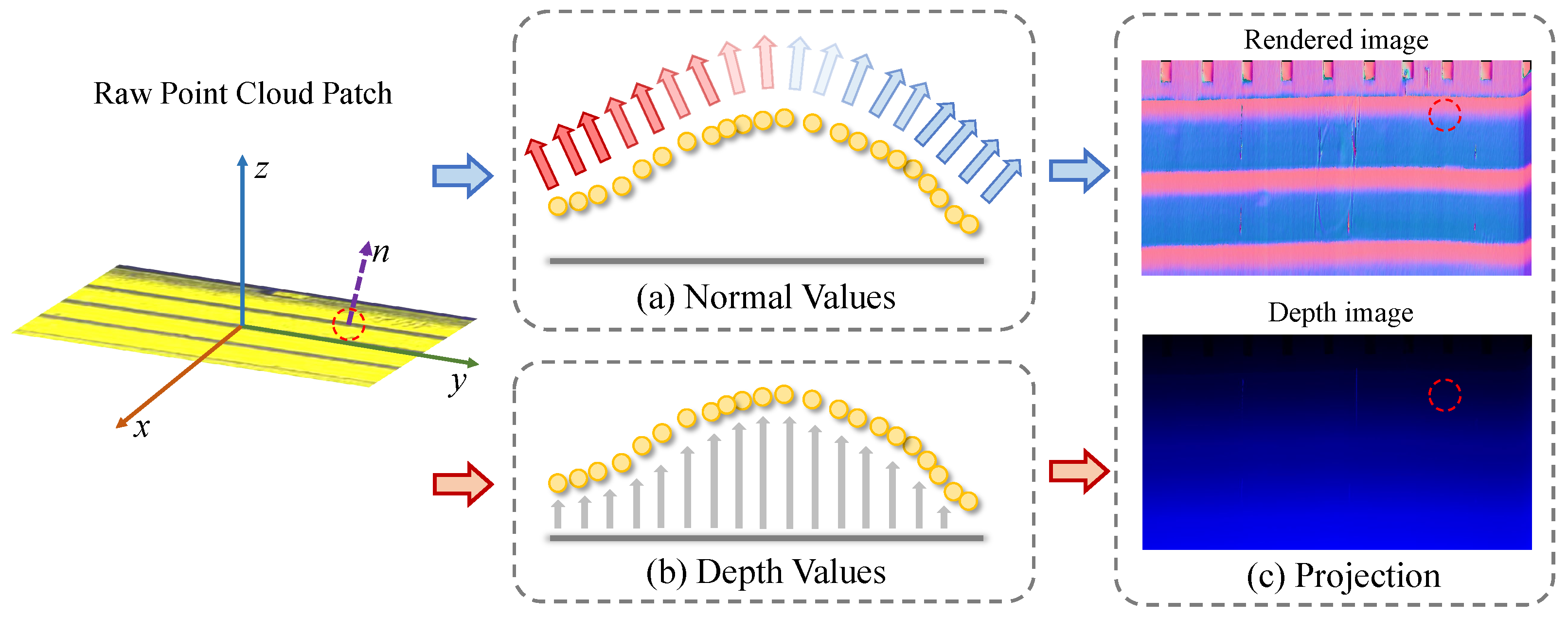
2.2. Normal-Based 3D Rendering

In this section, we elaborate on the normal-based rendering strategy for processing and extracting raw 3D surface data. By introducing point normals into the obtained feature map, we can estimate the surface orientations and search irregular bulge-like areas that contain rich information for subsequent detection. Then, in the rendering process, we combine the captured 3D information (normal and depth) and project it onto 2D planes for joint inputs from different domains.

• Surface normal estimation

The raw data captured by laser scanners are presented as depth information of parallel scanning lines. Intuitively, the obtained depth image (as shown in Figure 3c) is not ideal for defect detection because of the insignificant depth difference in local areas and inevitable noise. We first estimate geometric properties based on surface normals to extract accurate 3D surface characteristics from raw scans. In 3D geometry, a normal is one of the most fundamental properties that can effectively reflect the surface orientation of local regions. A surface normal at a point is a vector perpendicular to the surface around that point, as is shown in Figure 3a. Many different normal estimation techniques exist in the literature. Among them, one of the simplest methods is based on estimating the normal of a plane tangent to the surface.

Given a point cloud patch $\mathcal{P}\in {\mathbb{R}}^{N\times 3}$, we consider the neighboring points of each point $p\in \mathcal{P}$. We firstly employ an efficient Kd-tree to query neighboring points $\mathcal{K}=\left\{p_k\right|k\in \mathcal{N}\left(p\right)\}$ (p is included). Then, we use the least-square plane fitting estimation algorithm [13] to calculate the tangent plane t located at p. Following a previous study [13], the tangent plane t is represented by p and a normal vector n. We set c as an approximation of the centroid of neighboring points.

For estimating the normal vector n, we must analyze the $3\times 3$ covariance matrix A, which is written as

$$A=\frac{1}{\parallel \mathcal{K}\parallel }\sum _{p_k\in \mathcal{K}}(p_k-c){(p_k-c)}^T$$

(1)

where c is the centroid of neighboring points calculated by the mean of coordinates. By calculating the eigenvalues $v_j$ and eigenvectors $u_j$ ($j=0,1,2$) of A, we can obtain the smallest eigenvalue termed as $v_l={min}_{j\in \{0,1,2\}}{v}_j$, and the corresponding eigenvector $u_l$ is the approximation of n.

• Projecting 3D point clouds into 2D features

On the basis of the above two steps (i.e., preprocessing and normal estimation), we obtain the accurate depth information and surface geometric properties of each point in the local patches. Because of the difficulty of annotating 3D data and the heavy computational cost of neighbor searching in the 3D space, directly applying 3D detection models on raw point cloud data for inspecting tire defects is challenging [14,15,16]. To ease this problem, we intend to convert depth and normal information into regular 2D feature maps using a 3D projection strategy.

• Depth images

We first convert 3D point cloud data into regular grids according to camera parameters and scanning resolutions. The raw scan of a tire sample consists of several parallel scanning lines, each of which captures accurate depth values of different positions with a fixed resolution (see Figure 3). Therefore, we align the depth vectors and pad possible failure values with zero, which yields a regular 2D map with regard to the original scanning resolutions. By mapping the point-wise depth (i.e., the value of the z-axis) to the corresponding pixel, a projected depth image can be obtained, which significantly reduces the computational cost during detection. Moreover, as our scanner adopts fixed resolutions across the planer area, there is no information loss in depth channels between the 2D features and original 3D data.

• Rendered images

Similarly, we project point normals into pixel values arranged in a regular 2D feature map. Before projection, the global normal directions are reoriented toward the same direction by defining a virtual camera position outside the tire surface. The normal of each point possesses spatial coordinates represented as a 3D vector $(n_x,n_y,n_z)$. We normalize each channel and project the normalized values into RGB values to reduce information loss, which leads to a rendered image representing the tire surface directions in the 2D domain (as shown in Figure 3).

To facilitate annotation, we label defects with bounding boxes in the rendered images. Because of the projection property, the boxes in the rendered images and depth images are in one-to-one correspondence.

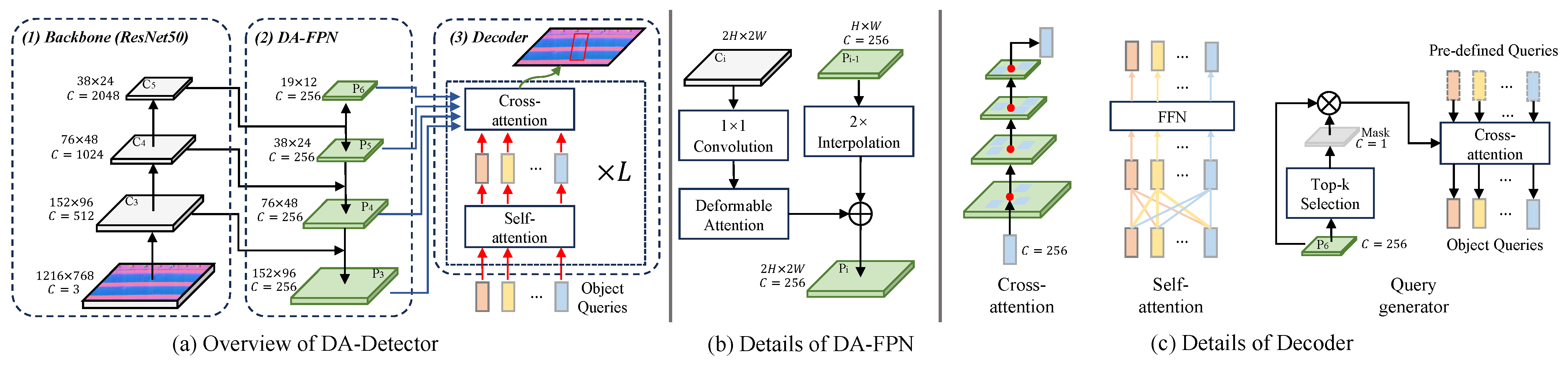
2.3. Attention-Based Detector

Inspired by the successful applications of transformers in 2D detection [8,9,17], we devise a novel attention-based detector that can effectively capture various forms of defects. The details of the proposed detector are illustrated in Figure 4.

• Deformable Attention

Applying vanilla-transformer-style attention on image feature maps necessitates looking over all spatial locations [9], which brings huge computational costs. To tackle this problem, we devise a deformable attention operation, where each pixel only needs to attend to its neighboring pixels. We follow the spirit of deformable convolutions [18,19] to enlarge the receptive field and capture long-range dependency, where each pixel can attend to its neighboring pixels in a large range with adaptive offsets. Specifically, given an input feature map $X\in {\mathbb{R}}^{C\times H\times W}$, let q denote the index of the query pixel with corresponding feature $x_q\in {\mathbb{R}}^C$ and 2D coordinate $p_q\in {\mathbb{R}}^2$, and the aggregated feature via deformable attention is calculated by

$$\mathrm{DeformAttn}(x_q,p_q)=\sum _{k=1}^K{A}_{qk}·W\left(x_{p_q+{\Delta }_{qk}}\right)$$

(2)

where k represents the index of the sampled key pixels and K is the total number of key pixels. Note that $K\ll HW$ for efficiency. ${\Delta }_{qk}$ and $A_{qk}$, respectively, denote the adaptive offset and attention weight of the kth sampling point. $A_{qk}$ is calculated by subtracting $x_q$ with $x_{p_q+\Delta p_{qk}}$, followed by a multilayer perceptron (MLP). Following a previous study [20], the value of $A_{qk}$ lies in the range $[0,1]$, which is normalized by the $\mathrm{softmax}$ function. Meanwhile, ${\Delta }_{qk}$ is obtained via linear projection over the query feature $x_q$ following a previous study [18]. As with deformable convolutions, $p_q+{\Delta }_{qk}$ is fractional; therefore, bilinear interpolation is applied in computing $x_{p_q+{\Delta }_{qk}}$. Note that our proposed deformable attention works like a deformable convolution but with adaptive weights determined by data.

• Defect Detector Based on the Proposed Deformable Attention

As shown in Figure 4a, following the spirit of detection with transformer (DETR) [9] and fully convolutional one-stage (FCOS) detection [21], our detector mainly consists of a domain adaptive (DA) feature pyramid network (FPN) and DA-decoder.

FPN [22] is one of the most important modules for detection. Following the top-down architecture of FPN, we replace the original $1\times 1$ convolution with deformable attention operation to capture local properties (as shown in Figure 4b), dubbed as DA-FPN.

With all pixels in the last feature map, we employ top-k selection to select object queries with the maximum activation value, which is adaptively generated by MLP. Then, we concat them with learnable queries [9] for object queries. The DA-decoder mainly consists of L DA-decoding blocks. There are cross-attention and self-attention modules in each block. In the cross-attention module, object queries extract features from the feature map, where the key elements are around the query pixels whose normalized coordinates are predicted by MLP. In each self-attention module, object queries interact with each other with the help of deformable attention without sampling. During training, we follow DETR [9] and utilize a bipartite matching algorithm to match GT and object queries.

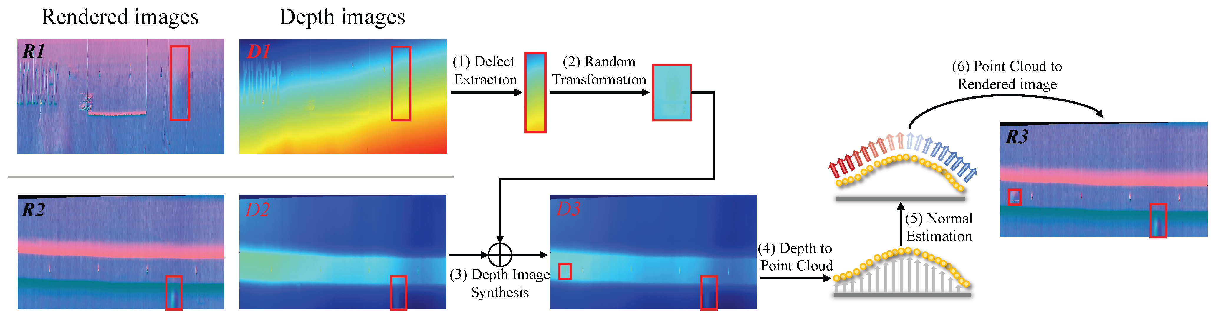
2.4. Data Augmentation

Obtaining a robust generalized deep detector using very little training data is impossible. However, because of various restrictions in industrial data collection, the size of the training dataset is small. Previous methods augmented datasets in trivial ways, such as rotation and flipping (see Figure 5). However, these previous methods brought limited benefits because of the following: (1) the number of defects remains unchanged because rotation or flipping cannot change the forms of defects; (2) the geometric transformation of images changes the tire texture and then leads to distortion; and (3) most existing methods are devised for classification tasks specifically and thus are not suitable for detection tasks.

To this end, we propose a novel approach of data augmentation, which can generate synthetic images with natural and diverse tire defects. The proposed data augmentation is devised for tiny defect detection tasks but can be extended to other detection tasks.

As aforementioned, one depth image has a corresponding rendered image, and both of them share a unified annotation. Generating synthetic depth images with defects is the first step of our data augmentation. According to the annotations, we first extract the tiny defects in depth images. Then, for each defect, we employ random deformation to obtain several defects with various forms. Lastly, by randomly choosing a template depth image (with or without defects), we synthesize a new depth image with automatically generated annotation.

The second step of data augmentation is to obtain rendered images from synthetic depth images. As shown in Figure 3, the projection from depth images to point clouds is easily accomplished without a loss of information, and normal vectors of point clouds are recalculated and projected to rendered images.

By repeating the above two steps of our data augmentation, a sufficient and nearly natural dataset is generated.

2.5. Details of the 3D Scanner

We used Banner LPM301-170 as the scanning device for collecting data. The sensing beam was a visible red laser, and the resolution was 1280 Pts/profile. The field of view ranged from 47 to 85 mm. The number of points in each contour line is 640. Please refer to the product manual, which can be downloaded from its official website, for more details about this 3D scanner. After scanning a tire, we can obtain a point cloud with around ${10}^8$ points.

3. Experiments and Discussion

In this section, we first evaluated the performance of our method compared with state-of-the-art tire defect detection approaches. A new 3D tire dataset was introduced, which was the first dataset using 3D data for the detection of low-visibility tire defects. Then, we compared our proposed 3D pipeline with existing defect-detection methods based on X-ray images. Afterward, based on the 3D tire dataset, we used four different data configurations to demonstrate the effectiveness of our proposed pipeline: point clouds, RGB images, depth images, and rendered images. Notably, in actual detection pipelines, our method used rendered images for detecting tire defects. Moreover, we provided several ablation studies on rendered images to analyze the important designs of our detection model. Finally, we analyzed some failure cases.

3.1. 3D Tire Dataset and Evaluation Metrics

As aforementioned, we proposed four types of datasets of tire defects: three 2D datasets (i.e., rendered images, depth images, and photoed RGB images) and one point cloud dataset. All datasets consisted of 880 training samples and 220 testing samples except for the RGB image dataset. RGB images were taken by 2D cameras, which hardly reflected the properties of the defects. Meanwhile, the point cloud dataset consisted of patches of the same sizes. Depth images and rendered images were generated using our 3D-to-2D approaches and augmented by our novel data augmentation, and the two corresponding images of these two datasets share the same annotations. Note that tire defect detection was not performed directly on point clouds because of the extremely high computational costs and low accuracy [23,24]. Instead, point clouds served as intermediate representations in data augmentation.

We trained all methods under standard settings on training datasets and evaluated them on testing datasets. We followed the evaluation metrics of the COCO dataset [25] and employed standard protocols to evaluate all methods on 2D datasets. Average precision (AP) is a popular metric in measuring the accuracy of object detectors and can be calculated as

$$AP=\left|classes\right|\sum _{c\in classes}\frac{T{P}_c}{F{P}_c+T{P}_c}.$$

(3)

Here, $\left|classes\right|$ refers to the number of categories. $T{P}_c$ and $F{P}_c$ are true positive and false positive bounding boxes, respectively, calculated by setting different thresholds of IoU. Specifically, AP₅₀ and AP₇₅ are calculated using the thresholds of 50% and 75%, respectively. $mAP$ is the mean AP with a threshold from 50% to 95% at a step size of 5%. AP${}_S$, AP${}_M$, and AP${}_L$ are used to evaluate the performance of detectors for objects with small, middle, and large sizes.

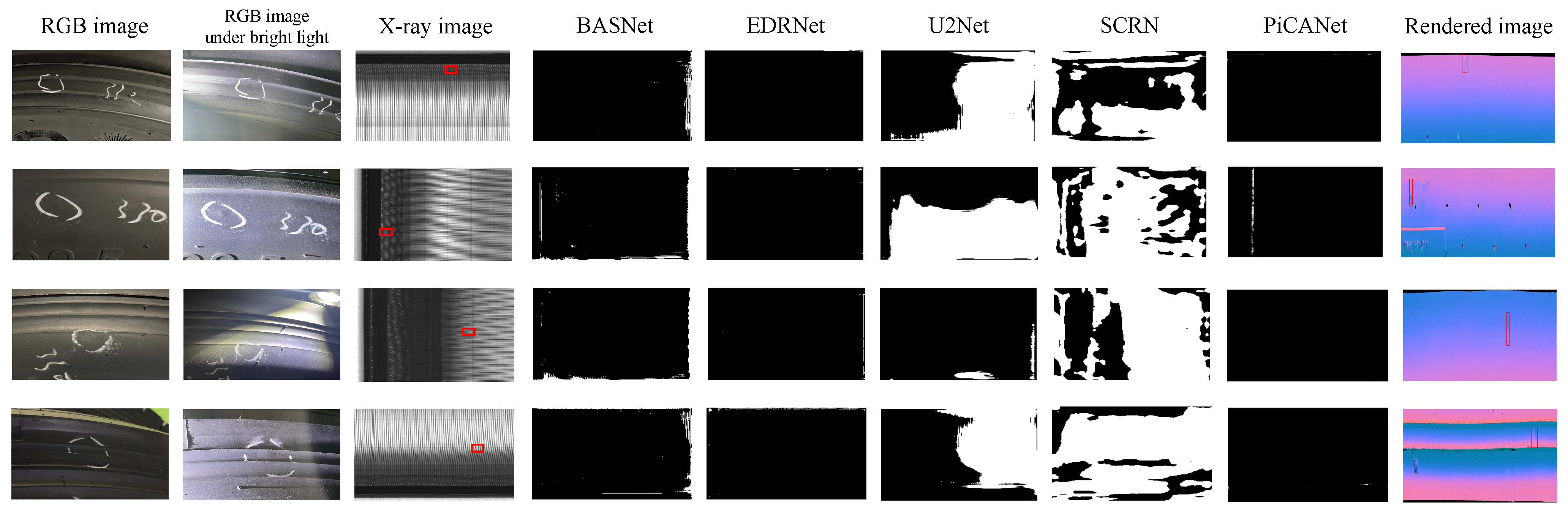
3.2. Comparison with X-ray-Based Methods

Mainstream methods formulate tire defect detection as a semantic segmentation task. Specifically, typical methods are based on X-ray images, and binary labels are predicted to identify defect areas. Although these methods have achieved successful results on several types of tire defects, we argue that they are not suitable for the inspection of bulge-like defects, as discussed in Section 1. The problems of these methods lie in the following: 1. Two-value masks are not suitable for practical defect detection, which requires clear marks such as bounding boxes instead of segmented pixels. 2. The annotation of segmentation datasets is time-consuming and laborious, making it hard to construct large-scale datasets. 3. Tiny defects are difficult to capture using X-ray scanners.

To justify the aforementioned observations, we captured additional X-ray images based on the tires used in the 3D tire datasets. As shown in the first column of Figure 6, unfortunately, identifying defects in these images is hard. We tested several state-of-the-art methods, including EDRNet [26], BASNet [27], U2Net [28], PiCANet [29], and SCRN [30], on our captured X-ray images. Qualitative results are shown in Figure 6, from which we can clearly find that locating defects from segmented results was hard, impeding practical applications.

3.3. Evaluation on the 3D Tire Dataset

In this section, we evaluated several state-of-the-art 2D detectors, including our model, on three tire defect datasets. In the development process of object detection, three mainstream methods have gradually emerged: anchor-based methods (Faster-RCNN [31]), anchor-free methods (FCOS [21] and RetinaNet [32]), and DETR-based methods (Deformable-DETR [8], DAB-DETR [33], and Conditional DETR [34]). Our proposed detector adopted the most advanced DETR-based architecture. The evaluation results are shown as follows.

• Implementation details

We used ImageNet [35] and pretrained ResNet-50 [36] as the backbone for all methods. For a fair comparison, all methods shared the same optimizer, scheduler, and epoch. The shared optimizer was an Adam optimizer [37] with a learning rate of $2\times {10}^{-4}$, ${\beta }_1=0.9$, and ${\beta }_2=0.999$ and a weight decay of ${10}^{-4}$. All models were trained for 100 epochs; the learning rate decayed at the 40th, 60th, and 80th epochs by a factor of 0.1. All experiments were conducted in 4 NVIDIA GEFORCE 1080 Ti graphic cards.

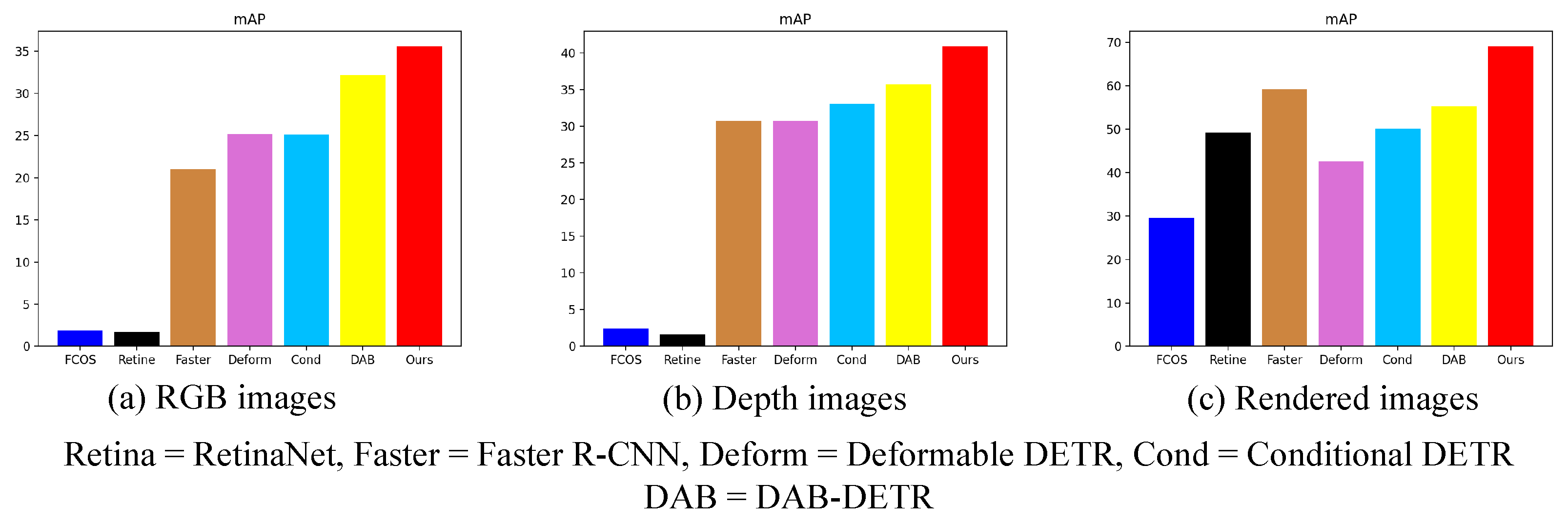
• Experiment on RGB images

We first conducted experiments on captured images using RGB cameras. As shown in

Table 1. Comparison of state-of-the-art methods on RGB images.

Methods	mAP	AP50	AP75	AP${}_{\mathit{S}}$	AP${}_{\mathit{M}}$	AP${}_{\mathit{L}}$
Faster R-CNN [31]	21.0	56.0	13.2	0.0	12.2	29.1
FCOS [21]	1.9	8.8	0.6	0.0	0.0	5.5
RetinaNet [32]	1.7	10.1	1.2	0.0	0.9	4.1
Deformable-DETR [8]	25.2	58.8	14.8	0.0	15.6	31.3
Conditional DETR [34]	25.1	59.2	13.2	0.0	15.8	32.0
DAB-DETR [33]	32.2	61.2	15.5	0.0	18.2	32.5
Ours	35.6	62.1	17.4	0.0	21.0	32.5

, our 2D detector outperformed state-of-the-art methods by a large margin. Compared with DAB-DETR [33], which achieved the second-best mAP, our detector improved mAP by 10.6%. However, because of the aforementioned drawbacks of 2D images, detecting such defects by human eyes is intrinsically difficult. Therefore, all detection methods performed unsatisfactorily, and all methods particularly failed to detect very tiny defects as ${\mathrm{AP}}_{\mathrm{S}}$ was 0. Anchor-free based FCOS [21] and RetinaNet [32] failed on this dataset. The evaluation results here indicate that photoed images are unsuitable for the detection of tiny defects.

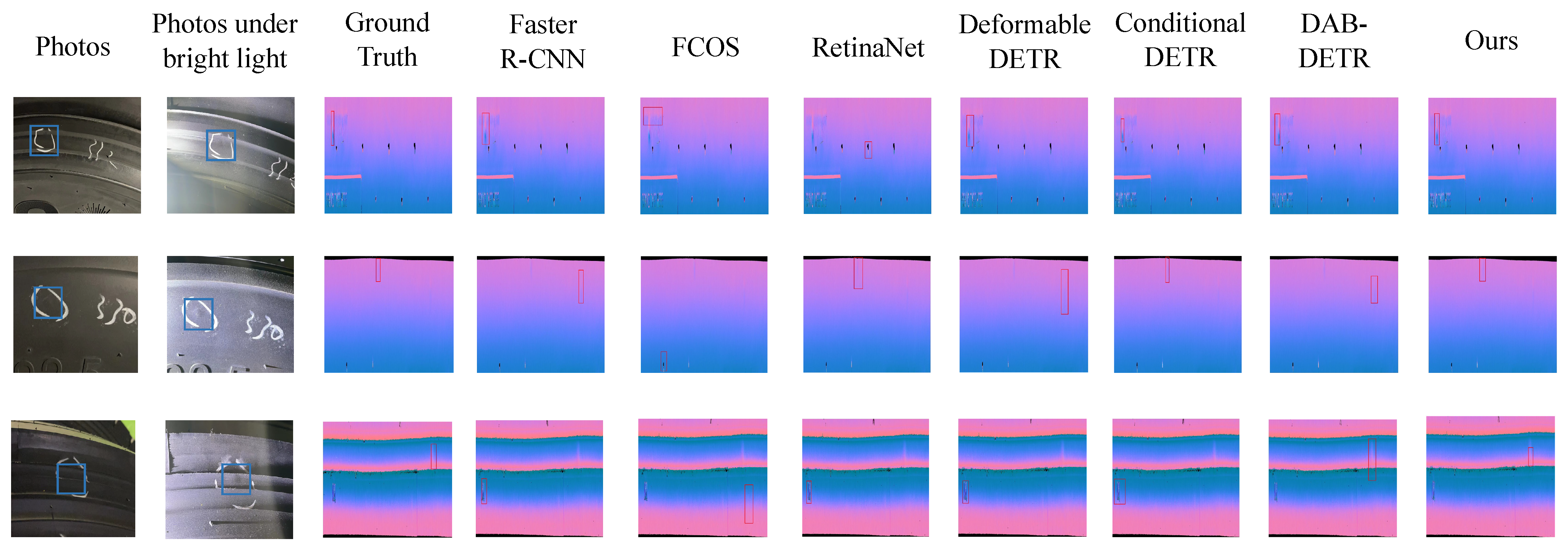
• Experiment on rendered images

We then experimented with rendered images. The quantitative results are shown in

Table 2. Comparison of state-of-the-art methods on rendered images.

Methods	mAP	AP50	AP75	AP${}_{\mathit{S}}$	AP${}_{\mathit{M}}$	AP${}_{\mathit{L}}$
Faster R-CNN [31]	59.2	89.8	65.5	23.6	52.8	73.0
FCOS [21]	29.6	73.0	21.1	0.7	28.0	37.5
RetinaNet [32]	49.2	87.4	50.0	7.1	47.3	60.0
Deformable-DETR [8]	42.5	88.6	39.6	8.3	29.9	72.0
Conditional DETR [34]	50.1	88.2	51.2	10.0	47.2	65.0
DAB-DETR [33]	55.3	88.4	63.2	18.3	52.0	70.2
Ours	69.1	89.8	74.1	35.7	59.2	89.6

in detail. Apparently, our method outperformed the other techniques by a large margin; specifically, our method achieved 0.691 mAP, which was 16.7% better than that of Faster R-CNN [31]. For defects with large sizes and medium sizes, our method achieved 0.896 ${\mathrm{AP}}_{\mathrm{L}}$ and 0.592 ${\mathrm{AP}}_{\mathrm{M}}$. In particular, for tiny defects, our method achieved 0.357 AP${}_S$, which was 51.3% better than that of the second-ranked Faster-RCNN, showing that our method is sensitive to tiny defects and promising in practical applications. The qualitative results are illustrated in Figure 7. For each method, we showed the bounding box with the highest confidence, which was colored in red. Many normal areas had similar patterns with defective areas, which confused the detection. For example, RetinaNet [32] identified the black burrs as defects in the first row. Faster-RCNN [31] recognized the normal bulge as a defective one. Thanks to several novel designs, our detector accurately detected the real defects, whereas other competitors failed in some cases.

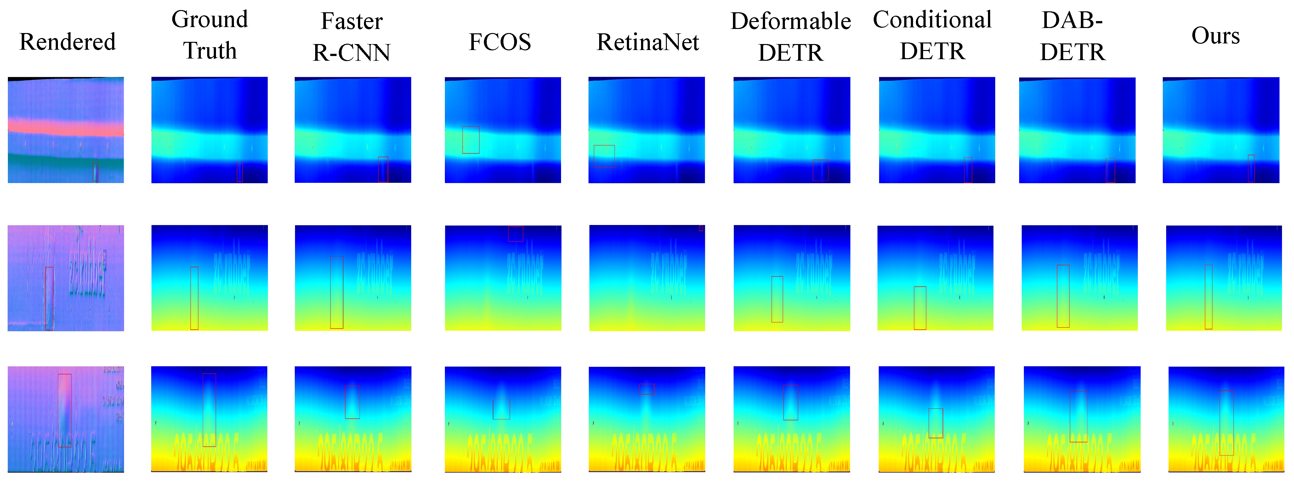
• Experiment on depth images

Lastly, we experimented on the depth image set. The quantitative results are shown in

Table 3. Comparison of state-of-the-art methods on depth images.

Methods	mAP	AP50	AP75	AP${}_{\mathit{S}}$	AP${}_{\mathit{M}}$	AP${}_{\mathit{L}}$
Faster R-CNN [31]	30.7	64.9	23.4	1.1	22.9	47.2
FCOS [21]	2.4	9.7	0.1	0.0	0.4	6.0
RetinaNet [32]	1.6	5.7	0.8	0.0	1.0	3.6
Deformable-DETR [8]	30.7	57.1	33.8	0.0	12.4	60.1
Conditional DETR [34]	33.1	65.0	33.4	0.0	13.0	59.2
DAB-DETR [33]	35.7	69.8	36.4	0.0	11.5	62.0
Ours	40.9	72.0	38.6	8.2	30.1	62.2

. The evaluation results clearly show that our detection method achieved much better results than those of other methods (14.5% better than that of the second-ranked DAB-DETR [8] in terms of mAP). In particular, our method achieved 0.082 ${\mathrm{AP}}_{\mathrm{S}}$, whereas other methods almost failed to detect tiny defects, indicating that our method can detect very tiny defects and justifying the novel designs of our detector. The qualitative results are shown in Figure 8. Similar to the experiment in the rendered image set, we visualized the top-1 bounding box of each method. The visual results further proved the advanced performance of our detector.

We show three bar charts of mAP in Figure 9. All models based on rendered images intuitively outperformed variants on the other two datasets, showing the superiority of the normal-based rendering strategy. Moreover, our detector outperformed other methods on the three proposed datasets by a large margin.

3.4. Ablation Studies

In this section, we conducted comprehensive experiments on the rendered image dataset to justify the effectiveness of our method. All the results are shown in

Table 4. Ablation study of several components of our proposed DA-Detector.

Methods	mAP	AP50	AP75	AP${}_{\mathit{S}}$	AP${}_{\mathit{M}}$	AP${}_{\mathit{L}}$
A: FPN [22]	68.7	89.7	73.9	34.0	59.2	89.4
B: DA-FPN	69.1	89.8	74.1	35.7	59.2	89.6
C: Random selection	48.0	86.0	50.0	7.1	48.0	59.0
D: Top-k selection	69.1	89.8	74.1	35.7	59.2	89.6
E: $L=1$	24.9	59.0	14.7	0.0	15.6	31.3
E: $L=1$	49.3	86.0	50.1	7.2	47.3	60.0
F: $L=3$	58.4	87.0	73.2	30.1	58.1	85.7
G: $L=4$	69.1	89.8	74.1	35.7	59.2	89.6

.

We first conducted experiments to justify the effectiveness of DA-FPN. In model A, we adopted vanilla FPN [22], while we used DA-FPN in model B. We can clearly find that model B outperformed model A in all metrics. In particular, model B achieved 0.357 ${\mathrm{AP}}_{\mathrm{S}}$, which was 5% better than that of model A, indicating that DA-FPN showed more sensitivity to tiny defects. Then, we compared different query generation strategies. Model C adopted random selection by randomly selecting query vectors and corresponding coordinates in the feature map. However, this approach caused the performance to drop a lot ($\mathrm{AP}$ drops 44% from 0.691 to 0.480), which justified the effectiveness of our proposed top-k selection. Lastly, we tuned the hyperparameter L, which is the number of DA-decoding blocks, and we can find that setting more blocks results in better performance. Considering the computational complexity, we set $L=4$ in practice.

As illustrated in Figure 10, some failure cases exist. One category is missing detection. When one defect is located at the center or edge of a tire pattern, capturing distinctive geometric features is hard, leading to missing detection. Another category is wrong detection. In this case, our method is confused by some normal areas whose patterns are similar to those of tire defects. Although our detector failed to make correct predictions in the former case (i.e., missing detection), the geometric features of tire defects can be distinguished by human eyes, as shown in Figure 10. The performance of our model was constrained by the small dataset due to the lack of original data. Therefore, we aim to collect more defect data to promote the performance of our model. To tackle the latter failure case (i.e., wrong detection), we intend to devise a more robust rendering approach to extract more distinguishing geometric features.

4. Conclusions

Existing methods mainly rely on X-ray images to detect tire defects with clear visual quality and, therefore, are insensitive to certain types of tire defects in the manufacturing process, especially challenging defect types with low visibility. Moreover, existing methods apply semantic segmentation approaches to locate defects. Therefore, slight false pixel predictions significantly impact the results of defect defection, hampering their deployment in actual production lines. To this end, we proposed a new tire defect detection pipeline by introducing 3D laser scanning technology into the inspection. We first captured scanned 3D tire surface data presented as 3D point clouds, which can effectively capture accurate depth distribution on the 3D surfaces. Our method proposes a novel normal-based rendering strategy for capturing accurate depth information and a 2D detector based on deformable attention for the accurate detection of tire defects.

Under standard experimental settings, our detector achieved 0.356, 0.409, and 0.691 mAP on RGB, depth, and rendered images, respectively. Compared with state-of-the-art 2D detection methods, our detector showed superior performance. The experimental results shed light on the application of tire defect detection in actual production lines. However, there are a few limitations, mainly in the following two aspects:

(1)

The performance of the model was constrained by the scale of training data. However, collecting a large number of data in a short time is hard because of the time-consuming annotation process. While our novel data augmentation eased the lack of training data, synthetic data are not as good as real data.

(2)

The normal-based rendering process consisted of reading point cloud data, normal estimation, and 3D-to-2D projection. Because of the large scale of tire point clouds (more than ${10}^8$ points) and high dependency on the CPU, the first two steps of the rendering strategy consumed most of the time, which was more than $90\%$ of the total time in detecting one tire.

Therefore, in future endeavors, we aim to focus on (1) collecting more real defect samples data and devising more robust data augmentation methods; and (2) reducing the time consumption of normal-based rendering process with optimized mechanisms (e.g., GPU-based normal estimation and parallel data reading).

References

1. Luo, Q.; Fang, X.; Liu, L.; Yang, C.; Sun, Y. Automated visual defect detection for flat steel surface: A survey. IEEE Trans. Instrum. Meas. 2020, 69, 626–644. [Google Scholar] [CrossRef]
2. Nikitin, S.; Shpeizman, V.; Pozdnyakov, A.; Stepanov, S.; Timashov, R.; Nikolaev, V.; Terukov, E.; Bobyl, A. Fracture strength of silicon solar wafers with different surface textures. Mater. Sci. Semicond. Process. 2022, 140, 106386. [Google Scholar] [CrossRef]
3. Chen, L.; Luo, R.; Xing, J.; Li, Z.; Yuan, Z.; Cai, X. Geospatial transformer is what you need for aircraft detection in SAR Imagery. IEEE Trans. Geosci. Remote Sens. 2022, 60, 1–15. [Google Scholar] [CrossRef]
4. Liu, L.; Ma, Z.; Zhu, M.; Liu, L.; Dai, J.; Shi, Y.; Gao, J.; Dinh, T.; Nguyen, T.; Tang, L.C.; et al. Superhydrophobic self-extinguishing cotton fabrics for electromagnetic interference shielding and human motion detection. J. Mater. Sci. Technol. 2023, 132, 59–68. [Google Scholar] [CrossRef]
5. Lin, G.; Liu, K.; Xia, X.; Yan, R. An efficient and intelligent detection method for fabric defects based on improved YOLOv5. Sensors 2022, 23, 97. [Google Scholar] [CrossRef] [PubMed]
6. Fang, B.; Long, X.; Sun, F.; Liu, H.; Zhang, S.; Fang, C. Tactile-based fabric defect detection using convolutional neural network with attention mechanism. IEEE Trans. Instrum. Meas. 2022, 71, 1–9. [Google Scholar] [CrossRef]
7. He, K.; Gkioxari, G.; Dollár, P.; Girshick, R. Mask R-CNN. In Proceedings of the IEEE International Conference on Computer Vision, Venice, Italy, 22–29 October 2017; pp. 2961–2969. [Google Scholar]
8. Zhu, X.; Su, W.; Lu, L.; Li, B.; Wang, X.; Dai, J. Deformable detr: Deformable transformers for end-to-end object detection. arXiv 2020, arXiv:2010.04159. [Google Scholar]
9. Carion, N.; Massa, F.; Synnaeve, G.; Usunier, N.; Kirillov, A.; Zagoruyko, S. End-to-end object detection with transformers. In Proceedings of the Computer Vision–ECCV 2020: 16th European Conference, Glasgow, UK, 23–28 August 2020; Proceedings, Part I 16; Springer: Berlin/Heidelberg, Germany, 2020; pp. 213–229. [Google Scholar]
10. Wu, Z.; Jiao, C.; Sun, J.; Chen, L. Tire defect detection based on faster R-CNN. In Proceedings of the Robotics and Rehabilitation Intelligence: First International Conference, ICRRI 2020, Fushun, China, 9–11 September 2020; Proceedings, Part II 1; Springer: Berlin/Heidelberg, Germany, 2020; pp. 203–218. [Google Scholar]
11. Wang, R.; Guo, Q.; Lu, S.; Zhang, C. Tire defect detection using fully convolutional network. IEEE Access 2019, 7, 43502–43510. [Google Scholar] [CrossRef]
12. Zheng, Z.; Zhang, S.; Yu, B.; Li, Q.; Zhang, Y. Defect inspection in tire radiographic image using concise semantic segmentation. IEEE Access 2020, 8, 112674–112687. [Google Scholar] [CrossRef]
13. Shakarji, C.M. Least-squares fitting algorithms of the NIST algorithm testing system. J. Res. Natl. Inst. Stand. Technol. 1998, 103, 633. [Google Scholar] [CrossRef] [PubMed]
14. Wang, Y.; Solomon, J.M. Object dgcnn: 3D object detection using dynamic graphs. Adv. Neural Inf. Process. Syst. 2021, 34, 20745–20758. [Google Scholar]
15. Lang, A.H.; Vora, S.; Caesar, H.; Zhou, L.; Yang, J.; Beijbom, O. Pointpillars: Fast encoders for object detection from point clouds. In Proceedings of the IEEE/CVF Conference on Computer Vision and Pattern Recognition, Long Beach, CA, USA, 15–20 June 2019; pp. 12697–12705. [Google Scholar]
16. Zhang, X.; Wan, F.; Liu, C.; Ji, R.; Ye, Q. Freeanchor: Learning to match anchors for visual object detection. Adv. Neural Inf. Process. Syst. 2019, 32, 1–9. [Google Scholar]
17. Dai, Z.; Cai, B.; Lin, Y.; Chen, J. Up-detr: Unsupervised pre-training for object detection with transformers. In Proceedings of the IEEE/CVF Conference on Computer Vision and Pattern Recognition, Nashville, TN, USA, 20–25 June 2021; pp. 1601–1610. [Google Scholar]
18. Dai, J.; Qi, H.; Xiong, Y.; Li, Y.; Zhang, G.; Hu, H.; Wei, Y. Deformable convolutional networks. In Proceedings of the IEEE International Conference on Computer Vision, Venice, Italy, 22–29 October 2017; pp. 764–773. [Google Scholar]
19. Zhu, X.; Hu, H.; Lin, S.; Dai, J. Deformable convnets v2: More deformable, better results. In Proceedings of the IEEE/CVF Conference on Computer Vision and Pattern Recognition, Long Beach, CA, USA, 15–20 June 2019; pp. 9308–9316. [Google Scholar]
20. Vaswani, A.; Shazeer, N.; Parmar, N.; Uszkoreit, J.; Jones, L.; Gomez, A.N.; Kaiser, Ł.; Polosukhin, I. Attention is all you need. Adv. Neural Inf. Process. Syst. 2017, 30, 1–11. [Google Scholar]
21. Tian, Z.; Shen, C.; Chen, H.; He, T. Fcos: Fully convolutional one-stage object detection. In Proceedings of the IEEE/CVF International Conference on Computer Vision, Seoul, Republic of Korea, 27 October–2 November 2019; pp. 9627–9636. [Google Scholar]
22. Lin, T.Y.; Dollár, P.; Girshick, R.; He, K.; Hariharan, B.; Belongie, S. Feature pyramid networks for object detection. In Proceedings of the IEEE Conference on Computer Vision and Pattern Recognition, Honolulu, HI, USA, 21–26 July 2017; pp. 2117–2125. [Google Scholar]
23. Zhou, Y.; Tuzel, O. Voxelnet: End-to-end learning for point cloud based 3D object detection. In Proceedings of the IEEE Conference on Computer Vision and Pattern Recognition, Salt Lake City, UT, USA, 18–23 June 2018; pp. 4490–4499. [Google Scholar]
24. Liu, C.; Gao, C.; Liu, F.; Liu, J.; Meng, D.; Gao, X. SS3D: Sparsely-supervised 3d object detection from point cloud. In Proceedings of the IEEE/CVF Conference on Computer Vision and Pattern Recognition, New Orleans, LA, USA, 18–24 June 2022; pp. 8428–8437. [Google Scholar]
25. Lin, T.Y.; Maire, M.; Belongie, S.; Hays, J.; Perona, P.; Ramanan, D.; Dollár, P.; Zitnick, C.L. Microsoft coco: Common objects in context. In Proceedings of the Computer Vision—ECCV 2014: 13th European Conference, Zurich, Switzerland, 6–12 September 2014; Proceedings, Part V 13; Springer: Berlin/Heidelberg, Germany, 2014; pp. 740–755. [Google Scholar]
26. Song, G.; Song, K.; Yan, Y. EDRNet: Encoder–decoder residual network for salient object detection of strip steel surface defects. IEEE Trans. Instrum. Meas. 2020, 69, 9709–9719. [Google Scholar] [CrossRef]
27. Qin, X.; Zhang, Z.; Huang, C.; Gao, C.; Dehghan, M.; Jagersand, M. Basnet: Boundary-aware salient object detection. In Proceedings of the IEEE/CVF Conference on Computer Vision and Pattern Recognition, Long Beach, CA, USA, 15–20 June 2019; pp. 7479–7489. [Google Scholar]
28. Qin, X.; Zhang, Z.; Huang, C.; Dehghan, M.; Zaiane, O.R.; Jagersand, M. U2-Net: Going deeper with nested U-structure for salient object detection. Pattern Recognit. 2020, 106, 107404. [Google Scholar] [CrossRef]
29. Liu, N.; Han, J.; Yang, M.H. Picanet: Learning pixel-wise contextual attention for saliency detection. In Proceedings of the IEEE Conference on Computer Vision and Pattern Recognition, Salt Lake City, UT, USA, 18–23 June 2018; pp. 3089–3098. [Google Scholar]
30. Wu, Z.; Su, L.; Huang, Q. Stacked cross refinement network for edge-aware salient object detection. In Proceedings of the IEEE/CVF International Conference on Computer Vision, Seoul, Republic of Korea, 27 October–2 November 2019; pp. 7264–7273. [Google Scholar]
31. Ren, S.; He, K.; Girshick, R.; Sun, J. Faster R-CNN: Towards real-time object detection with region proposal networks. Adv. Neural Inf. Process. Syst. 2015, 28, 1–9. [Google Scholar] [CrossRef] [PubMed]
32. Lin, T.Y.; Goyal, P.; Girshick, R.; He, K.; Dollár, P. Focal loss for dense object detection. In Proceedings of the IEEE International Conference on Computer Vision, Venice, Italy, 22–29 October 2017; pp. 2980–2988. [Google Scholar]
33. Liu, S.; Li, F.; Zhang, H.; Yang, X.; Qi, X.; Su, H.; Zhu, J.; Zhang, L. Dab-detr: Dynamic anchor boxes are better queries for detr. arXiv 2022, arXiv:2201.12329. [Google Scholar]
34. Meng, D.; Chen, X.; Fan, Z.; Zeng, G.; Li, H.; Yuan, Y.; Sun, L.; Wang, J. Conditional detr for fast training convergence. In Proceedings of the IEEE/CVF International Conference on Computer Vision, Montreal, QC, Canada, 10–17 October 2021; pp. 3651–3660. [Google Scholar]
35. Deng, J.; Dong, W.; Socher, R.; Li, L.J.; Li, K.; Li, F.-F. Imagenet: A large-scale hierarchical image database. In Proceedings of the 2009 IEEE Conference on Computer Vision and Pattern Recognition, Miami, FL, USA, 20–25 June 2009; pp. 248–255. [Google Scholar]
36. He, K.; Zhang, X.; Ren, S.; Sun, J. Deep residual learning for image recognition. In Proceedings of the IEEE Conference on Computer Vision and Pattern Recognition, Las Vegas, NV, USA, 27–30 June 2016; pp. 770–778. [Google Scholar]
37. Kingma, D.P.; Ba, J. Adam: A method for stochastic optimization. arXiv 2014, arXiv:1412.6980. [Google Scholar]
Figure 1. (a) Tire bubble defects, a major defect type usually inspected by experienced workers using additional light sources. We show that this type of defect is difficult to detect in X-ray (b) or RGB (c) images because of its low visual quality. (d) shows the data used in our method, presented as 3D point clouds and then converted into rendered 2D images (e) for subsequent detection. Red frames indicate the locations of defects.
Applsci 13 11350 g001
Figure 2. Overview of the proposed architecture for tire defect detection. (a) shows our mechanical environment where a laser scanner is installed to capture 3D point clouds on tire surfaces. (b) denotes the training phase of our method, which combines a normal-based 3D rendering process and a 2D detection model. (c) shows the testing phase where our method predicts results based on rendered images.
Applsci 13 11350 g002
Figure 3. Projection process from raw 3D data to 2D feature maps. By extracting pointwise depth and normal values, our method projects input 3D point clouds onto 2D planes, which can capture depth and surface orientation information. Red circles indicates the defects.
Applsci 13 11350 g003
Figure 4. Our detector based on the proposed deformable attention. (a) DA-Detector consisting of a backbone (ResNet50), DA-FPN, and a decoder. (b) Details of DA-FPN, where deformable attention operation is used to replace the vanilla 1 × 1 convolution. (c) Cross-attention mechanism is used to extract the features of DA-FPN with object queries. With a self-attention mechanism, object queries interact with each other. For query generation, we use a top-k selection strategy instead of vanilla learnable queries.
Applsci 13 11350 g004
Figure 5. Diagram of the proposed data augmentation. Red frames indicate the defects. R i and D i are the corresponding rendered and depth images, sharing the same annotation. The data augmentation mainly consists of six steps: (1) extracting defect from the annotated depth images; (2) applying a random transformation to generate a novel defect; (3) integrating the generated defect into another depth image; (4) recovering a point cloud based on the synthetic depth map; (5) reestimating the normal; and (6) obtaining a new rendered image with 3D to 2D projection.
Applsci 13 11350 g005
Figure 6. Visual comparison of previous defect-detection methods for tire bubble defects from the 3D dataset. Red frames indicate the defects. We show that existing X-ray-based approaches are insensitive to this type of defect because of its low visual quality.
Applsci 13 11350 g006
Figure 7. Visual comparison of rendered images. Red frames indicate the defects. We show the bounding box with maximum confidence for each method. Images are scaled for typesetting.
Applsci 13 11350 g007
Figure 8. Visual comparison of depth images. Red frames indicate the defects. We show the bounding box with maximum confidence for each method. Images are scaled for typesetting.
Applsci 13 11350 g008
Figure 9. Bar charts of mAP on three datasets.
Applsci 13 11350 g009
Figure 10. Illustration of failure cases. Failure cases can be classified as missing and wrong detection cases.
Applsci 13 11350 g010