STRP-DBSCAN: A Parallel DBSCAN Algorithm Based on Spatial-Temporal Random Partitioning for Clustering Trajectory Data

Abstract

Trajectory clustering algorithms analyze the movement trajectory of the target objects to mine the potential movement trend, regularity, and behavioral patterns of the object. Therefore, the trajectory clustering algorithm has a wide range of applications in the fields of traffic flow analysis, logistics and transportation management, and crime analysis. Existing algorithms do not make good use of the temporal attributes of trajectory data, resulting in a long clustering time and low clustering accuracy of spatial-temporal trajectory data. Meanwhile, the density-based clustering algorithms represented by DBSCAN are very sensitive to the clustering parameters. The radius value Eps and the minimal points number MinPts within Eps radius, defined by the user, have a significant impact on the clustering results, and tuning these parameters is difficult. In this paper, we present STRP-DBSCAN, a parallel DBSCAN algorithm based on spatial-temporal random partitioning for clustering trajectory data. It adopts spatial-temporal random partitioning to distribute balanced computation among different computing nodes and reduce the communication overhead of the parallel clustering algorithm, thus improving the execution efficiency of the DBSCAN algorithm. We also present the PER-SAC algorithm, which uses deep reinforcement learning to combine the prioritized experience replay (PER) and the soft actor-critic (SAC) algorithm for autotuning the optimal parameters of DBSCAN. The experimental results show that STRP-DBSCAN effectively reduces the clustering time of spatial-temporal trajectory data by up to 96.2% and 31.2% compared to parallel DBSCAN and the state-of-the-art RP-DBSCAN. The PER-SAC algorithm also outperforms the state-of-the-art DBSCAN parameter tuning algorithms and improves the clustering accuracy by up to 8.8%. At the same time, the proposed algorithm obtains a higher stability of clustering accuracy.

1. Introduction

Trajectory data are one of the most classical types of spatial-temporal data. Due to the scale, dynamics, and multi-source heterogeneity of the data, spatial-temporal trajectory data contain a lot of potential key information. By clustering and analyzing spatial-temporal trajectory data, the hidden patterns and laws in the trajectories can be discovered, which can then guide important decision-making and optimization. Therefore, the clustering of spatial-temporal trajectory data has important application value in the fields of traffic flow regulation [1], route planning [2], and disease prediction [3].

Traditional clustering algorithms have been widely used for trajectory data. The division-based clustering algorithm represented by K-Means [4] is simple and easy to use, but it is sensitive to the selection of the initial center of mass and K-value. The computational overhead of such algorithms is too high when dealing with high-dimensional data and they do not perform well when dealing with non-spherical data. Density-Based Spatial Clustering of Application with Noise [5] (DBSCAN) is a typical density-based clustering method that determines the clustering results based on the distribution of the data samples. It automatically determines the number of final clusters without pre-setting and can cluster dense datasets of arbitrary shape with low sensitivity to outliers. These properties make DBSCAN the preferred algorithm for many clustering problems, and it has a robust performance in many areas such as financial analysis [6] and business research [7]. However, DBSCAN is still mainly used on spatial data in trajectory clustering. The ST-DBSCAN [8] algorithm adds the consideration of temporal attributes to the traditional DBSCAN algorithm for clustering spatial-temporal data. TSBC algorithm [9], which is based on the trajectory segmentation fitting model, accomplishes clustering by adopting different fitting models to segment the trajectory data and aggregate the segmented data. Current clustering algorithms, especially DBSCAN and its derivatives, still have many shortcomings in clustering spatial-temporal trajectory data. On the one hand, when the dataset is large, the convergence time of DBSCAN to perform clustering is long. On the other hand, DBSCAN is more sensitive to the parameters, in which the two global parameters, radius value Eps and the minimal points number MinPts within Eps radius, have a significant impact on the final clustering results. It is difficult to tune the parameters compared to the traditional algorithms such as K-Means.

The RP-DBSCAN algorithm [10] is one of the best for clustering large-scale spatial-temporal trajectory data. It achieves approximate load balancing on different computing nodes by using the idea of approximate processing, dividing the data into cells and performing pseudo-random partitioning based on the cells. However, the RP-DBSCAN algorithm is still essentially based on clustering spatial data, and therefore it does not make good use of the temporal attribute information contained in the spatial-temporal trajectory data. In this paper, we present STRP-DBSCAN, a parallel DBSCAN algorithm based on spatial-temporal random partitioning for clustering trajectory data. STRP-DBSCAN is an improvement on the RP-DBSCAN algorithm. It assigns data that are close in both the spatial and temporal attributes to the same partition as far as possible for computation by introducing temporal partitioning based on the idea of the spatial random partitioning of RP-DBSCAN. In this way, STRP-DBSCAN can further improve the efficiency of clustering spatial-temporal data and speed up the clustering computation. Aiming at the problem that DBSCAN is more sensitive to the global parameters, we propose a PER-SAC algorithm based on deep reinforcement learning (DRL), which automatically tunes the optimal parameters to improve the clustering accuracy.

The contributions of this paper are summarized as follows:

• The STRP-DBSCAN algorithm is proposed, by introducing the idea of spatial-temporal random partitioning, data that are close in spatial and temporal attributes are divided into the same partition as far as possible to achieve a better load balancing among different computing nodes, which reduces the communication of parallel computation and improves the clustering efficiency.
• The DRL-based PER-SAC algorithm is proposed to solve the parameter sensitivity problem of DBSCAN, which uses the prioritized experience replay (PER) mechanism combined with the soft actor-critic (SAC) algorithm to construct an optimal parameters autotuning framework for DBSCAN in a simple, fast, and efficient way.
• The proposed algorithm is extensively evaluated on the acquired real dataset of public automatic identification system (AIS), and the experimental results show that the proposed algorithm effectively improves the clustering speed and clustering accuracy of the spatial-temporal trajectory data and achieves a better stability of the clustering results.

The rest of this paper is organized as follows. Section 2 introduces related work. Section 3 presents the STRP-DBSCAN algorithm. Section 4 describes the implementation of the PER-SAC algorithm. Section 5 shows the evaluation results. Section 6 concludes this paper.

2. Related Work

Clustering is one of the most widely used data analysis and mining methods, conducted by measuring the similarity between objects and classifying those with a high degree of similarity into the same category. Clustering algorithms can be categorized into five main groups. The division-based clustering algorithms, such as K-means [8] and K-Medoids [11], use a few human-defined points as the initial centroids, and iteratively cluster until all data points are clustered based on heuristics. This class of algorithms is more sensitive to outlier points. The hierarchical-based clustering algorithms, such as BIRCH [12] and CURE [13], calculate the distance between the samples and combine the closest points until the clustering is completed. These algorithms have a high time complexity. The grid-based clustering algorithms divide the data space into grid cells, then map the data to the grid cells and calculate the density of each cell, and the neighboring dense cells form a cluster, such as STING [14] and CLIQUE [15]. But in general, they suffer from a lower accuracy. The model-based clustering algorithms mainly refer to probabilistic model-based methods and neural network model-based methods, such as GMM [16] and SOM [17]. They have a high computational complexity and poor clustering effect when the amount of data is small. In addition, the density-based clustering algorithms, such as DBSCAN [5] and OPTICS [18], check the continuity between samples in term of sample density and continuously expand the clusters based on connectable samples to obtain the final clustering results. Among them, the DBSCAN algorithm does not need to specify the number of clusters and can cluster datasets of arbitrary shapes, which is a classical clustering algorithm that has been widely used in many research fields, such as traffic flow mining, business center location selection, etc. However, existing clustering algorithms are not efficient to deal with the special properties of spatial-temporal trajectory data such as multi-dimensionality, large data volume, and high sparsity. For example, the classical DBSCAN algorithm is only applicable to spatial clustering, and the effect of clustering spatial-temporal trajectory data with multi-dimensional attribute information such as time is unsatisfactory.

Recently, a number of research works have emerged to cluster spatial-temporal trajectory data. The ST-DBSCAN algorithm [8] processes and analyzes the data from the temporal and spatial dimensions, respectively. But the algorithm is more sensitive to the relevant parameters than the DBSCAN algorithm. And it fails to closely combine the temporal and spatial attributes of the trajectory data for clustering. The Quick Bundles clustering algorithm [19] can effectively process the spatial-temporal data and converge quickly. However, the selection of the clustering thresholds has a large impact on the final result of this algorithm, which relies heavily on manual experience setting. The MDST-DBSCAN algorithm [20] realizes the clustering of high-dimensional spatial-temporal data, but the selection of the initial point of clustering will have a great influence on the clustering results, so the stability of this algorithm is poor. In general, the existing spatial-temporal trajectory data clustering algorithms, especially the DBSCAN-based algorithms, have optimizable space in clustering efficiency when dealing with large-scale high-dimensional data. At the same time, such algorithms are sensitive to the Eps and MinPts parameters, and the clustering accuracy and efficiency are often limited by the optimization of clustering parameters.

Parallelization is one of the most commonly used methods to accelerate the clustering speed of trajectory data. Parallel DBSCAN [21], the earliest distributed parallel version of the DBSCAN algorithm, realizes parallelization through the distributed spatial indexing data structure dR*-Tree to achieve an approximate linear speedup effect. But it is difficult to deal with large scale trajectory data. Prokopenko et al. proposed a new framework [22] for GPU acceleration of DBSCAN and designed two tree-based algorithms to update clustering information by fusing neighborhood search, which achieves a good performance on low-dimensional data but underperforms on high-dimensional data. The RP-DBSCAN algorithm [10] was proposed based on the Spark parallel framework. It solves the problem of load imbalance between data partitions to a large extent through the pseudo-random partitioning based on cells and greatly improves the speed of the algorithm compared with the ordinary parallel DBSCAN algorithm, but it is only suitable for processing spatial data.

The DBSCAN-based algorithms have a high sensitivity to parameters, and the accuracy of clustering results usually depends on the clustering parameters chosen based on experience. Recently, a lot of work has been conducted on adaptive or automated methods to determine the optimal parameters of DBSCAN. Among them, the DSets-DBSCAN algorithm [23] is to find the optimal parameter of Eps by fixing a MinPts value, and therefore, it is not fully intelligent. The AA-DBSCAN algorithm [24] adopts a new tree structure based on a quadtree to define the density layer of the dataset, but it still needs to input the relevant parameters. The KANN-DBSCAN algorithm [25] is based on a cyclic iterative optimization strategy, which generates the candidate Eps and MinPts parameter sets according to the distribution characteristics of dataset. The algorithm has a long runtime and requires manual selection for the acquired optimal parameter sets. The MOGA-DBSCAN algorithm [26] selects the parameters based on the multi-objective genetic algorithm, but it still has problems such as a long running time and the need for parameter tuning when facing large-scale data.

In recent years, deep reinforcement learning (DRL) [27] has been well applied in parameter optimization by virtue of its integration of the powerful comprehension ability of deep learning [28] in perceptual problems and the decision-making ability of reinforcement learning [29], which enables it to make more accurate decisions in complex environments [30]. For example, a DRL-based DBSCAN algorithm [31] uses the TD3 [32] as the core algorithm to build an adaptive DBSCAN parameter tuning framework. We denote this DRL-based algorithm as TD3-DBSCAN in this paper to distinguish our proposed algorithm. Since the TD3 algorithm involves many parameters that have an impact on the performance, such as the learning rate and the update frequency of target network, a large number of experiments and debugging are required, and the stability of the obtained optimal parameters is poor. The maximum entropy principle-based method tends to allow the intelligent agent to learn a random strategy that enables it to explore more behaviors in the scenarios with multiple optimal or sub-optimal behaviors. Therefore, the soft actor-critic (SAC) algorithm [33], a deep reinforcement learning algorithm based on the maximum entropy principle and the actor-critic framework, has the advantages of high stability, wide exploration space, and less influence by parameters.

At the same time, DRL algorithms such as DQN [34] adopt the experience playback mechanism as a random sampling method with equal probability, which can ensure that each experience can be well sampled and learned by the agent. However, different experiences have different impacts on policy optimization, and the random sampling approach ignores the importance of high-value experiences. The prioritized experience replay (PER) [35] differentiates the importance of experience and prioritizes the sampling of high-value experience, which allows it to better optimize the strategy and improve the stability and efficiency of the algorithm.

Therefore, based on the state-of-the-art DBSCAN algorithm, this paper proposes the STRP-DBSCAN algorithm by introducing the idea of spatial-temporal partitioning, which provides a better and more balanced distribution and clustering of the trajectory data in the temporal attributes and effectively speeds up the execution of the algorithm without affecting the accuracy. In this work, we also combine the advantages of the SAC algorithm and the PER mechanism and propose the DRL-based adaptive parameter autotuning algorithm PER-SAC, which provides stable optimal parameters for STRP-DBSCAN to improve the clustering accuracy of the algorithm for spatial-temporal trajectory data.

3. STRP-DBSCAN

3.1. Background Knowledge

DBSCAN finds the directly density-reachable relationship from a data point p, located at the core of a dense region, to a data point q to form a cluster of the maximal set of data points connected by this relationship. To implement parallel DBSCAN, a cell-based grid structure is used to split the entire dataset into regions for parallel computing.

According to [5,10], there are some preliminaries to understand. There are two parameters in DBSCAN that need to be defined in advance, i.e., the radius of a neighborhood ε and the minimal points number MinPts within ε. The data space of the entire d-dimensional data points is portioned into a grid consisting of many equal-sized cells, and each cell is a d-dimensional hypercube with diagonal length ε. If the number of neighborhood points of data point p is not less than MinPts, p is a core point and it can represent a dense region. A point q is directly density-reachable from a core point p if the Euclidean distance between p and q is less than or equal to ε. A point q is density-reachable from a point p if a sequence of points p₁, p₂, …, p_n exists such that p = p₁ ∧ q = p_n ∧ ∀iЄ[1, n-1]: p_i+1 is directly density-reachable from p_i. A cell C is considered as a core cell if at least one core point exists within C. When C₁ and C₂ are both core cells, p and q are the core points of C₁ and C₂, respectively, if the Euclidean distance between p and q is less than or equal to ε, then C₂ (C₁) is fully directly reachable from C₁ (C₂). When C₁ is a core cell and C₂ is not a core cell, if the Euclidean distance between the core point p of C₁ and a data point q of C₂ is less than or equal to ε, then C₂ is partially directly reachable from C₁. Figure 1 shows the density reachability between cells.

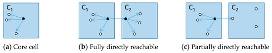
Figure 1. Density reachability between cells.

3.2. RP-DBSCAN

The proposed STRP-DBSCAN is an improvement version of RP-DBSCAN. As a state-of-the-art fast parallel DBSCAN algorithm, based on the cell-level reachability, RP-DBSCAN [10] contains three main phases.

3.2.1. Data Partition

This phase is divided into two parts, i.e., pseudo-random partitioning and cell dictionary building. Data points read from the Hadoop distributed file system (HDFS) are first partitioned into a data space of cells, and pseudo-random partitioning is then performed on the cells. A cell in the d-dimensional data space can be further divided into 2^d(h−1) sub-cells with diagonal length ε/2^h−1, where $h=1+⌈{\log }_2(1/\rho )⌉$ and ρ is a parameter that determines the size of a sub-cell. In addition, ε also corresponds to the Eps parameter in DBSCAN. If at least one core point exists, it is guaranteed that all data points in the cell where the data point is located belong to the same clustering, which greatly improves the efficiency of the subsequent merging of the local clustering results, compared with the ordinary distributed DBSCAN algorithm. By giving each cell a random key value, cells with the same key value will be assigned to the same computing node.

RP-DBSCAN also employs a two-level cell dictionary data structure that can be viewed as a two-level KD-tree, where the root node in the first level is used to encode cells and the leaf nodes in the second level are used to encode sub-cells. Each entry of the node keeps a record of the location of the corresponding (sub)cell and the number of data points it contains. Such a structure represents the entire dataset in the form of an overall summary, which is broadcast to each computing node, thus reducing the communication overhead between computing nodes and the storage space occupation on each node. Figure 2 shows the building of the two-level cell dictionary.

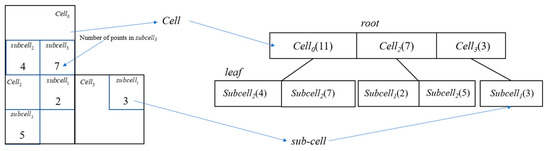
Figure 2. Building process of the two-level cell dictionary in RP-DBSCAN.

3.2.2. Cell Graph Construction

This phase consists of two parts, core cell labeling and cell graph construction. Each computing node simultaneously calculates the density reachability relationship within the partition, i.e., with the help of two-level cell dictionary to perform an (ε, ρ)-region query on the data points within each partition. The (ε, ρ)-region query counts the data points contained within the ε-neighborhood of the data point and labels the cell where the data point is located as the core cell if the sum is more than or equal to MinPts.

Figure 3 shows an example of (ε, ρ)-region query. The data space in Figure 3 contains 4 cells and each cell contains 16 sub-cells. It is assumed that the diagonal length of each cell is $4\sqrt{2}$, i.e., ε is $4\sqrt{2}$, and ρ is 0.25. In the (ε, ρ)-region query of the data point D₁, the number of data points contained in the region is 11. If the MinPts is set to 7, the data point D₁ will be labeled as a core point and the cell C₁ where D₁ is located will be labeled as a core cell.

Figure 3. Illustration of (ε, ρ)-region query.

Next, using the cell as the smallest unit, the cell graph in the partition is obtained by searching for fully or partially density-reachable cells from each core cell and aggregating the local clustering results within each partition by adding directed edges. A cell graph is defined as G = (V, E), where vertices are cells and edges are reachability relationships between cells. Since a cell graph is constructed from a single computing node, here we call it a sub-cell graph to distinguish from the cell graph for the entire dataset. The type of directed edges (fully or partially density-reachable) between cells cannot be conclusively confirmed as there may be cases where a cell is assigned to other partitions during this phase.

3.2.3. Cell Graph Merging

In this phase, the algorithm will merge the sub-cell graphs generated by each node to generate a new cell graph, i.e., merging the local clusters and labeling the final clustering results. In the process of subgraph merging, the direction of fully density reachable edges will not have an effect on the final merging result, so the computational redundancy between core cells can be eliminated by eliminating the direction of fully reachable edges. When eliminating redundant edges, the cell graph is merged using a two-by-two approach to obtain the final cell graph.

Each subgraph can specify whether the cells in its own partition are core or non-core cells, so in each pairwise merging, the two sub-level cell graphs can obtain more information about data points and edges, and some previously undetermined cells can be reconfirmed as core or non-core. For two given cell graphs G₁ and G₂ which merge into a single cell graph G₁∪G₂, as the types of the cells in G₁∪G₂ are updated, the types of the edges also need to be updated. In addition, to ensure that we obtain correct clustering results as the normal DBSCAN, we assign the same label to data points with the same cluster_id.

Figure 4 uses an example to illustrate the three main phases of RP-DBSCAN. Since the cell C₁ is labeled as a non-core cell in Figure 4b, it will be excluded in the next phase of cell graph construction in Figure 4c. Figure 4d illustrates the expansion of the clusters in the process of cell graph merging.

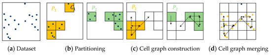
Figure 4. Three main phases of RP-DBSCAN.

The overall execution flow of RP-DBSCAN is shown in Figure 5.

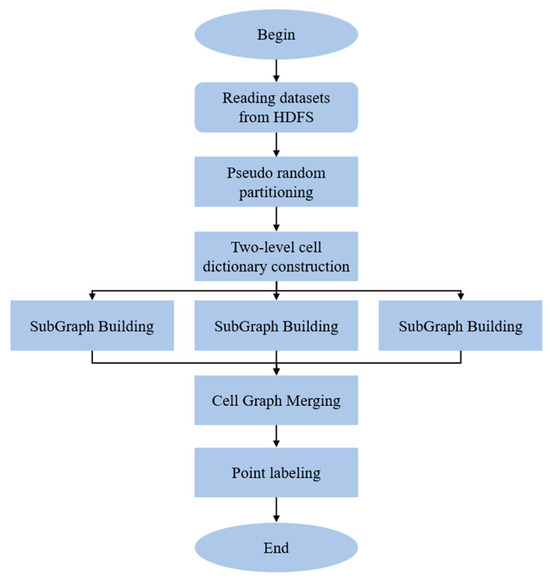
Figure 5. Overall execution flow of RP-DBSCAN.

3.3. Overview of STRP-DBSCAN

The STRP-DBSCAN algorithm is an improved version of RP-DBSCAN, introducing spatial-temporal random partitioning to improve the load balancing of spatial-temporal trajectory data. The acquired spatial-temporal data are first preprocessed by STRP-DBSCAN to reduce the influence of the noisy data on the subsequent calculation of the algorithm. Based on the idea of partitioning, STRP-DBSCAN uses the spatial-temporal random partitioning processing to randomly select the time information of the data points in each cell as the partition key of the cell, and cells with the same partition key will be assigned to the same partition, which realizes the load balancing of the spatial-temporal data and further improves the clustering efficiency of spatial-temporal data. The other phases are similar to RP-DBSCAN. The overall execution flow of STRP-DBSCAN is shown in Figure 6.

Figure 6. Overall execution flow of STRP-DBSCAN.

3.4. Preprocessing of Spatial-Temporal Trajectory Data

Each spatial-temporal trajectory data contains information in multiple dimensions, such as object ID, latitude and longitude, velocity, direction, time, etc. Due to the presence of noise and error in the acquired raw spatial-temporal data, the data should be preprocessed to ensure the rationality of the data, which can effectively reduce the impact of the noisy data on the subsequent calculations of the algorithm.

Taking ship trajectory data as an example, the ship class spatial-temporal trajectory dataset mainly relies on the collection of data reports continuously sent by shipboard AIS equipment. The time interval when shipboard AIS equipment continuously send data reports will be different, i.e., in the same period of time, the different ship AIS reports are prone to redundancy, so for the same ship, one data point can be selected within each minute for approximation.

In this paper, the main process of the preprocessing of spatial-temporal trajectory data is as follows:

• First, removing the points that do not conform to regular speeds, have missing values for certain attributes, and have irregularities in latitude and longitude;
• Constructing key-value pairs with ID as the key and time as the value in the dataset. For different categories of trajectory data, setting the smallest time measurement unit according to the specific situation;
• Removing data elements in the dataset where both ID and time are the same, i.e., removing the redundant data;
• Normalizing the data in terms of latitude, longitude, precision, and time, i.e., eliminating the effect of magnitude on subsequent clustering.

The normalization can limit the preprocessed data to a certain range, thus eliminating the adverse effects caused by singular sample data. Since normalization only scales the data and does not change the original information of the data, there is no loss of information. In this work, we use the most commonly used max–min normalization, as shown in Equation (1).

$$x\text{'}=\frac{x-x_{\min }}{x_{\max }-x_{\min }}$$

(1)

3.5. Spatial-Temporal Random Partition

The most significant improvement of STRP-DBSCAN compared to RP-DBSCAN is the spatial-temporal random partition based on the spatial and temporal information contained in the trajectory data, respectively. In the spatial dimension, each data point is assigned to the cell and sub-cell to which it belongs according to its positional coordinates in each dimension. Meanwhile, in the time dimension, the time value of the data point in each cell is randomly selected as the partition key for that cell, and cells with the same partition key will be assigned to the same partition. The algorithm stores the information about the data points in the cells, as well as the sub-cells in a two-level cell dictionary, i.e., a general summary of the dataset, and sends it to each computing node by broadcasting, which enables different computing nodes to achieve local clustering despite not knowing the complete dataset. The implementation of the spatial-temporal random partitioning is shown in Algorithm 1.

Algorithm 1. Spatial-Temporal Random Partition

Input: dataset D containing N data points, radius parameter Eps, minimal points number within the radius MinPts, number of partitions k, approximation parameter rho Output: cells {C1,C2,...}, cell dictionary M, partition data {P1,…Pk} 1  //Spatial-Temporal Randomization Partition 2    class Spatial_Time_Pseudo_Random_Partitioning(D, Eps, rho, k) 3  //Assign points to different cells 4     method MAP(NULL, point p) 5         cid = the cell id of point p; 6         EMIT(cid, p); 7   //Partition according to time 8     method REDUCE(cid, {p1, p2,...}) 9          C = {p1, p2,...}; 10        pid = random(time in C); 11        EMIT(pid, C); 12    method REDUCE(pid, {C1, C2,...}) 13        newPpid = {C1, C2,...}; 14        EMIT(pid, newPpid); 15   //Cell dictionary construction 16   class CELL_DICTIONARY_BUILDING({P1,...Pk}, Eps, rho) 17       method MAP(pid, newPpid) 18          for each Ci∈newPpid do 19            Ci = {sc1, sc2,...}; 20          newMpid = make a cell dictionary; 21          EMIT(NULL, newMpid); 22       method REDUCE(NULL, newM1, newM2,..., newMk) 23         $M=new{M}_1\cup new{M}_1\cup \cdots \cup new{M}_k$; 24         EMIT(NULL, M);

Figure 7 shows an example of spatial-temporal partition. Due to the normalization, values for all dimensional attributes of the data are in the range [0, 1]. All data points are mapped into a 3D data space of cells, as shown in Figure 7a. Cells of different colors are distributed to different computing nodes. Although the partition is performed in 3D data space, the 2D plan view consisting of the time axis and the latitude axis allows for a more intuitive and obvious demonstration of the data partitioning. Figure 7b shows the original data point distribution in the 2D plan of the time axis and the latitude axis, and Figure 7c shows the partition results of Figure 7b. Cells that contain data points at the same height in the time axis but differ in the latitude axis are assigned to the same partition.

Figure 7. Illustration of spatial-temporal random partition.

3.6. Implementation of STRP-DBSCAN

The phases of cell graph construction and cell graph merging in STRP-DBSCAN are similar to those in RP-DBSCAN. The pseudo-code implementation of STRP-DBSCAN is shown in Algorithm 2.

Algorithm 2. STRP-DBSCAN

Input: Dataset D containing N data points, Eps, MinPts, number of partitions k, approximation parameter rho. Output: Data with clustered labels. 1   //Phase I: Data Partitioning. 2   //Partitioning of data using spatial-temporal randomization. 3     {P1,…,Pk} = Spatial_Time_Pseudo_Random_Partitioning(D,Eps,rho,k); 4   //Cell dictionary construction. 5     M = Cell_Dictionary_Building({P1,…,Pk},Eps,rho); 6   //Inform the constructed cell dictionary to each node in the distributed environment via broadcasting. 7     Cell_Dictionary_Broadcasting(M); 8   //Phase II: Cell map construction (local clustering). 9   //Core cell labelling and subgraph construction. 10   {G1,…,Gk} = Core_Marking_and_Subgraph_Building({P1,…,Pk},Eps,MinPts); 11  //Phase III: Cell map merging (merged clustering). 12  //Subgraph merging. 13    newG = Progressive_Graph_Merging({G1,…,Gk}); 14  //Labelling the points. 15    newD = Point_Labelling({P1,…,Pk}, newG); 16    return newD;

The computational complexity of STRP-DBSCAN mainly comes from the cell graph construction phase, i.e., the (ε, ρ)-region query in each partition to find candidate cells via the two-level cell dictionary. Therefore, the complexity is O (log|cell|), where |cell| is the maximum number of cells among all partitions. The complexity of STRP-DBSCAN is the same as that of RP-DBSCAN. However, the |cell| of STRP-DBSCAN is smaller than that of RP-DBSCAN because STRP-DBSCAN introduces spatial-temporal random partitioning, which achieves a more balanced partitioning of the dataset among computing nodes. Theoretically, STRP-DBSCAN has a lower computational complexity than RP-DBSCAN.

4. PER-SAC based Optimal Parameter Autotuning for DBSCAN

4.1. PER-SAC Algorithm

The PER-SAC algorithm combines the SAC algorithm with the PER mechanism to fast search the stabilized optimal parameter for DBSCAN. The SAC algorithm is a DRL algorithm of the actor-critic type considering maximum entropy, which increases the exploration degree of the DRL model by adopting a more stochastic strategy, exhibiting excellent performance on both discrete action tasks and continuous action tasks.

The experience playback mechanism has been used in many DRL algorithms such as TD3 and SAC. However, different experiences do not have the same value to the DRL agent and have different impacts on the strategies. But the uniform random sampling ignores, to some extent, those experiences with high values that can better optimize the strategies. Based thereon, this paper adopts the prioritized experience playback mechanism on the basis of uniform sampling of the experience replay buffer of the SAC algorithm to construct a DRL framework for the parameter autotuning of DBSCAN.

The PER mechanism first uses the value of the time-difference deviation (TD-error) of each experience, i.e., the absolute value of the difference between the Target_Q value and the Current_Q value, as an index to evaluate the value of the experience. The larger the absolute value of the TD-error, the more important the experience to be learned by the agent. The experiences in the experience replay buffer are sorted in order of their value. Multiple sampling and playback are possible for certain high-value experiences. In addition, the bias problem due to changes in the sample distribution is solved by the importance sampling weight (ISW).

In the preliminary “warm-up” phase of the algorithm, the agent adopts an exploration strategy to interact with the environment, obtaining random samples and storing them in the experience buffer until enough samples have been stored in the experience buffer. When starting training, the PER-SAC algorithm first samples according to the weights and draws batch_size size samples from the prioritized experience replay buffer. The algorithm calculates the TD-error of each sample separately based on the drawn samples and obtains the loss values of each network based on the individual network loss function J_Q(θ), J_π(φ), J(α). The loss functions of Q-network Q(θ), the strategy π(φ), and the weighting factor α are shown in Equations (2)–(4), respectively, where E is the expectation function and $\stackrel{-}{H}$ is the minimum expected entropy of the expectation. The parameter explanation of Equations (2)–(4) is listed in Table 1.

$$\begin{array}{l}{J}_Q(\theta )=E_{(s_t,a_t)~D}[\frac{1}{2}{w}_t(Q_{\theta }(s_t,a_t)-(r(s_t,a_t)+\\ E_{s_{t+1}~p}(s_{t+1}\left|s_t,a_t\right.)[\gamma {\pi }_t{(s_{t+1})}^T(Q_{\overline{\theta }}(s_{t+1},a_{t+1})-\alpha log({\pi }_{\phi }(a_{t+1}\left|s_{t+1}\right.)))]{)}^2]\end{array}$$

(2)

$$J_{\pi }(\phi )=E_{s_t~D}[w_t{\pi }_t{(s_t)}^T[\alpha log({\pi }_{\phi }(s_t))-Q_{\theta }(s_t)]]$$

(3)

$$J(\alpha )=w_t{\pi }_t{(s_t)}^T[-\alpha (log({\pi }_{\phi }(s_t))+\overline{H})]$$

(4)

Table 1. Parameter explanation of equations.

Parameters	Explanation
st	State of the environment at the moment t
at	The action performed by the agent at the moment t
rt	Feedback on the action at performed by the agent in the state st of the moment t
θ	Q network parameter
φ	Policy network parameter
α	Weighting factor
w	Importance sampling weight
γ	Discount factor

Each network updates its corresponding network parameters according to the above loss functions. When all the samples in a batch_size are trained, the PER-SAC algorithm updates the latest priorities to the corresponding samples in the prioritized experience replay buffer. The DRL network structure based on PER-SAC is shown in Figure 8.

Figure 8. DRL network structure based on PER-SAC.

The pseudo-code of the PER-SAC algorithm is shown in Algorithm 3.

Algorithm 3. PER-SAC Algorithm

Input: Q-network parameters ${\theta }_1$, ${\theta }_2$, policy-network parameter $\phi$ Output: ${\theta }_1^{*}$, ${\theta }_1^{*}$, ${\phi }^{*}$ 1  Initialize Q-network parameters ${\theta }_1$, ${\theta }_2$, policy-network parameter 2  Initialize Q-network parameters 3  $\overline{{\theta }_1}\leftarrow {\theta }_1$, $\overline{{\theta }_2}\leftarrow {\theta }_2$ 4  //Initializing an empty PER experience replay buffer D 5    $D\leftarrow \varnothing$ 6    for each iteration do 7        for each environment step k = 1…T do 8               $a_t~{\pi }_{\phi }\left(a_t|s_t\right)$ //Sample action from the policy 9               $s_{t+1}~p\left(s_{t+1}\right|s_t,a_t)$//Sample transition from the environment 10             $D\leftarrow D\cup \{s_t,a_t,r\left(s_t,a_t,s_{t+1}\right),s_{t+1}\}$//Store the transition in the replay buffer 11        end for 12     if $D$.capacity > warmup size then 13            for each gradient step do 14                //Sample samples S, sample indices indices, weights w from D 15                 $S,indices,w~D$ 16                 $J_Q=J_Q^S$//Loss function for the Q-network 17                 $J_{\pi }=J_{\pi }^S$//Loss function for the policy network 18                 $J_{\alpha }=J_{\alpha }^S$//Loss function for the weighting factor α 19                ${\theta }_i\leftarrow {\theta }_i-w{\lambda }_Q {\widehat{\nabla }}_{{\theta }_i} J_Q\left({\theta }_i\right) i\in \left\{\mathrm{1,2}\right\}$//Update the Q-network parameters 20                 $\phi \leftarrow \phi -w{\lambda }_{\pi }{\widehat{\nabla }}_{\phi } J_{\pi }\left(\phi \right)$ //Update the policy network parameters 21                 $\alpha \leftarrow \alpha -w\lambda {\widehat{\nabla }}_{\alpha } J_{\alpha }$ //Adjust temperature factor 22                 $\overline{{\theta }_i}\leftarrow \tau {\theta }_i+\left(1-\tau \right)\overline{{\theta }_i} i\in \left\{\mathrm{1,2}\right\}$ //Update Target network weights 23                 $p\leftarrow \left|{\delta }^S\right|$//Update the prioritization of samples 24            end for 25        end if 26   end for

4.2. Optimal Parameter Autotuning Framework

The PER-SAC algorithm is used to build an optimal parameter autotuning framework for DBSCAN. The process of finding the optimal parameters of DBSCAN can be regarded as a maze game problem in a finite parameter space, where the initial parameters are iteratively autotuned by training the agent and interacting with the environment until the optimal parameters are obtained.

The agent regards the parameter space and the DBSCAN algorithm as the environment, the result obtained by the clustering algorithm as the state, and the direction of parameter tuning as the action, and it performs iterative optimization. In addition, we use a small number of samples (i.e., 20% of the original dataset) to reward the agent with superior performance in a weakly-supervised manner and optimize the policy functions of the agent based on the PER-SAC framework.

The overall structure of the optimal parameter autotuning framework based on the PER-SAC algorithm in a single episode is shown in Figure 9. The actor network selects the action a_t to be executed based on the current state s_t. The state of the environment is transformed s_t+1 to after executing the action a_t, and inputs (s_t, a_t) into the critic network for scoring to calculate the reward r_t. Then, the current experience (s_t, a_t, s_t+1, r_t) is stored into the PER buffer. During subsequent training, experiences are selected and learned from this buffer based on prioritization for updating the parameters of the network and tuning the parameter set of {Eps, MinPts}. The framework performs in this manner until reaching the parameter boundaries or the upper limit of the number of searches, and the search process for this episode ends.

Figure 9. Parameter autotuning process of the framework in a single episode.

For the reward function used in the parameter autotuning framework, we use 20% of samples to provide an external measure of the effect of clustering and as a basis for reward. We define the immediate reward function of the i-th step as Equation (5).

$$R(s^{(e)(i)},a^{(e)(i)})=NMI(DBSCAN(X,P^{(e)(i+1)}),y\text{'})$$

(5)

Here, s^(e)(i) and a^(e)(i) indicate the state and action of the i-th step of the e-th episode, respectively. NMI () is the normalized mutual information (NMI) representing the external metric function of DBSCAN clustering. X is the feature set and y’ is the set of partial labels of the data block. NMI is commonly used to measure the accuracy of the results of clustering algorithms and we use it as the reward function. Furthermore, the optimal parameter search action sequence for an episode is to tune the parameters in the direction of the optimal parameters and stop the search at the optimal parameters. Therefore, we consider using the maximum immediate reward of subsequent steps and the endpoint immediate reward as the reward of i-th step, see Equation (6).

$$r^{(e)(i)}=\beta \cdot \max \{R(s^{(e)(m)},a^{(e)(m)})\}{|}_{m=i}^I+\delta \cdot R(s^{(e)(I)},a^{(e)(I)})$$

(6)

Here, R(s^(e)(I), a^(e)(I)) is the immediate reward for the I-th step end point parameter. And the max function is used to calculate the future maximum immediate reward before stopping the search in the current episode. β and δ are the impact factors of reward, where β = 1 − δ.

The process of parameter search is repeated for each recursive layer in the training process to optimize the agents, and the optimal parameter set of {Eps, MinPts} is updated based on the reward function. An early stopping mechanism is used to speed up the model training process while the optimal parameter set remains unchanged. When the same parameters are obtained more than three consecutive times, the training is aborted, which in turn speeds up the training process. While in the testing process, the trained agent is directly used to search in the batch, and the early stopping mechanism is no longer used. The parameters of the last layer after executing an episode can be used as the optimal parameter set. Algorithm 4 shows the optimal parameter autotuning process of the framework for DBSCAN.

Algorithm 4. Optimal parameter autotuning process for DBSCAN

Input: The features of dataset X, partial labels y’ of data block V; Agents for each layer: $\left\{agen{t}^{\left(l\right)}\right\}{|}_{l=1}^{L\max }$; Output: Optimal parameter set: P0; 1    for l = 1,…,Lmax do 2         //Initalize parameter space 3           Initialize the space boundaries of parameter p in the l-th layer $B_{p,1}^{(l)}$、 $B_{p,2}^{\left(l\right)}$, the search precision of the parameter p in the l-th layer ${\theta }_p^{\left(l\right)}$; 4           for e = 1,…,Emax do 5                 //Initalize parameter set 6                   Initalize $P^{\left(e\right)\left(0\right)}$ by $P_o^{(l-1)}$; 7                 //Parameter autotuning 8                   for i = 1,..., Imax do 9                         Obtain the current state s(e)(i); 10                         Choose a(e)(i) = Actor(s(e)(i)); 11                         get $p^{\left(e\right)\left(i\right)}\stackrel{a^{\left(e\right)\left(i\right)},\theta }{\to }{p}^{\left(e\right)(i+1)}$; 12                         DBSCAN($p^{(e)(i)}$); 13                         Termination judgment; 14                     end for 15                     if is TRAIN then get rewards 16                         $r^{(e)(i)}=\beta \cdot \max \{R(s^{(e)(m)},a^{(e)(m)})\}{|}_{m=i}^I+\delta \cdot R(s^{(e)(I)},a^{(e)(I)})$; 17                         Store ${\Gamma }^{(e)(i)}=(s^{(e)(i)},a^{(e)(i)},s^{(e)(i+1)},r^{(e)(i)})$ in experience replay buffer; 18                         Sampling and learning; 19                     end if 20                   //Update optimal parameter set $P_o^{(l)}$ 21                     update $P_o^{(l)}$; 22                     Early stop judgment; 23            end for 24            update $P_o$; 25            Early stop judgment; 26    end for

Regarding the computational complexity of parameter search, for ease of presentation, we define π_p to be the number of searchable parameters in the parameter space of parameter p in each layer. Additionally, ${\theta }_p^{\left(l\right)}$ is the search step size in the l-th layer, which can be defined as Equation (7).

$${\theta }_p^{(l)}=\left\{\begin{array}{c}\frac{{\theta }_p^{(l-1)}}{{\pi }_p}, \mathrm{if} p=Eps;\\ \max \{⌊\frac{{\theta }_p^{(l-1)}}{{\pi }_p}+\frac{1}{2}⌋,1\}, \mathrm{otherwise}.\end{array}\right.$$

(7)

Thus, the computational complexity is O (N) when there is no recursive structure, where $N={\theta }_p^{\left(0\right)}/{\theta }_p^{\left(L\right)}=({\pi }_p{)}^L$. Our optimal parameter autotuning framework with an L-layer recursive structure simply takes $L·\left({\pi }_p\right)$, reducing the complexity from O (N) to O (log N).

5. Experiments

5.1. Experiment Settings

1.

Dataset

The experiments use ship trajectory data to validate the proposed algorithms. The adopted dataset is the real ship data of public AIS in the East China Sea [36]. Since the proposed STRP-DBSCAN algorithm first preprocesses the dataset, for the real AIS dataset, the abnormal data points with a sailing speed of less than 2 knots and greater than 60 knots are removed, and the minute is set as the smallest time measurement unit. After preprocessing, two kinds of labeled datasets and unlabeled datasets are obtained, respectively. It is worth stating that the spatial-temporal trajectory clustering algorithm proposed in this paper is also applicable to other types of trajectory data.

2.

Evaluation metrics

The experiments will evaluate the algorithm in terms of both clustering efficiency and clustering accuracy. We evaluate the efficiency of the clustering algorithm in terms of the overall time it takes to obtain the final clustering results. At the same time, there are many common metrics that can be used to evaluate the goodness of the clustering results, i.e., clustering accuracy. For unlabeled data, we use the silhouette coefficient [37] and the Davies–Bouldin index [38] to evaluate clustering accuracy. For labeled data, we use the normalized mutual information (NMI) [39] and the adjusted Rand index (ARI) [40] for clustering accuracy measurement. Among them, except for the DBI index, the larger the value of the other three evaluation indexes, the better the clustering effect. For the execution efficiency of the algorithm, we used 10 runs of the algorithm and averaged the running time to evaluate the execution efficiency of the algorithm.

3.

Experimental configuration

The STRP-DBSCAN is a distributed parallel clustering algorithm based on the Spark implementation. The experimental information is shown in Table 2.

Table 2. Experimental configurations of STRP-DBSCAN.

Hardware/Software	Parameters
CPU	Intel®® Core™ i5-10400F CPU @ 2.90 GHz
Hadoop	Hadoop3.2
JDK	JDK 1.80_211
Scala	Intel AVX512
# of cores	12
Spark	Spark-3.1.3
Memory	32 GB DDR4
Operation system	CentOS Linux release 7.9.2009 (Core)

Table 3 shows the experimental information about the optimal parameter autotuning framework. For all baseline algorithms used in the experiments, the open-source implementation libraries or those provided by the authors were used and the experiments were conducted in the following environments.

Table 3. Experimental configuration of the PER-SAC algorithm-based framework.

Hardware/Software	Parameters
CPU	12th Gen Intel®® Core™ i7-12700H 2.30 GHz
PyTorch	Version 1.12.1
CUDA	Version 11.3
GPU	NVIDIA GeForce RTX 3070Ti
Python	Version 3.7.16

5.2. Evaluation of STRP-DBSCAN

The proposed STRP-DBSCAN algorithm is first evaluated. In this part of the experiments, we use three unlabeled datasets of size 8.5K, 50K, and 217K after preprocessing and normalization, respectively. We compared STRP-DBSCAN with the DBSCAN algorithm [5] and one of state-of-the-art parallel DBSCAN algorithms, i.e., RP-DBSCAN [10]. These two algorithms do not optimize the spatial-temporal data by preprocessing. To be fair, we uniformly use the preprocessed and normalized datasets for the experiments. In order to exclude any influence on the results, all tested algorithms used the same clustering parameters, i.e., Eps is set to 0.02 and MinPts is set to 100 for all datasets. For the three datasets of different data sizes, Table 4 records the computation time of the three clustering algorithms. If not specified, the experimental results in this paper are the average of ten executions.

Table 4. Execution time (s) of different algorithms with different data sizes.

Algorithms	8.5K	50K	217K
DBSCAN [5]	0.643	13.290	349.520
RP-DBSCAN [10]	4.456	6.089	19.327
STRP-DBSCAN	4.350	5.651	13.290

According to Table 4, the parallel algorithms RP-DBSCAN and STRP-DBSCAN algorithms are far less efficient than the ordinary DBSCAN algorithm when on the 8.5K dataset. This is because the parallel DBSCAN algorithm adds the process of data partitioning, merging clustering and other processes that require the communication of different computing nodes compared to ordinary DBSCAN algorithm, which increases the time overhead in the case of small dataset. However, as the dataset size gradually increases, the performance advantages of the parallel DBSCAN algorithms appear. On the 50K and 217K datasets, the overall execution time of STRP-DBSCAN is reduced by 57.5% and 96.2% compared with DBSCAN in the current experimental environment. Compared with RP-DBSCAN, the clustering time of STRP-DBSCAN on the 8.5K, 50K, and 217K datasets is improved by 2.4%, 7.2%, and 31.2%, respectively. The experimental results show that the algorithm based on spatial-temporal random partitioning can achieve a more balanced partitioning and effectively reduce the communication overhead between nodes, which improves the overall execution efficiency of the parallel clustering algorithm. It is also consistent with the previous algorithmic complexity analysis of STRP-DBSCAN.

Table 5 shows the evaluation result of the clustering accuracy of three algorithms on the same datasets. According to the results, STRP-DBSCAN has little or no impact on the clustering accuracy compared to DBSCAN and RP-DBSCAN. Combined with previous experimental results related to the clustering time, it shows that STRP-DBSCAN can improve the clustering efficiency for large data size, and the improvement becomes more obvious as the data size increases.

Table 5. Evaluation of clustering results using different algorithms with different data sizes.

Algorithms	8.5K		50K		217K
	DBI	Silhouette Coefficient	DBI	Silhouette Coefficient	DBI	Silhouette Coefficient
DBSCAN [5]	0.553	0.981	0.186	0.970	0.460	0.939
RP-DBSCAN [10]	0.548	0.981	0.186	0.971	0.461	0.936
STRP-DBSCAN	0.552	0.982	0.187	0.971	0.461	0.934

5.3. Evaluation of PER-SAC

In this part of experiments, we verify the effect of the proposed PER-SAC algorithm on the clustering accuracy of DBSCAN. Since the PER-SAC-based parameter autotuning framework for DBSCAN uses NMI as the reward function, it requires labeled datasets for searching the optimal clustering parameters. Therefore, in this part of experiments, we use labeled datasets of two sizes, 3.3K and 8.5K.

5.3.1. Selection of Hyper-Parameters

Considering that DRL algorithms such as TD3 and SAC are somewhat randomized, the experimental results are the means as well as the standard deviations after 10 different random seed runs. The parameter autotuning framework for DBSCAN involves other hyperparameters not related to the DBSCAN algorithm, such as the size of the parameter space [41], the reward factor, and the number of recursive layers of the model, which will also have an impact on the final clustering effect, and thus it is necessary to carry out the hyperparameter selection first.

We use the experimental method of empirical search to select the appropriate hyperparameters. Figure 8 demonstrates the effects of the parameter space size of Eps(π_Eps), the parameter space size of MinPts (π_MinPts), the number of recursive layers of the DRL network, and the reward factor on the performance of the framework. As shown in Figure 10, the results indicate that the parameter space is set too large or too small, which will result in a decrease in the final clustering effect or a decrease in the parameter searching efficiency. Moreover, an appropriate number of recursive layers, i.e., appropriate model size, and appropriate reward factor both help to obtain a stable clustering result and a high parameter searching efficiency. According to the experimental results, the experimental hyperparameters are chosen such that the parameter space size of Eps is set to 5, the parameter space size of MinPts is set to 4, the number of recursive layers is set to 3, and the reward factor is set to 0.2.

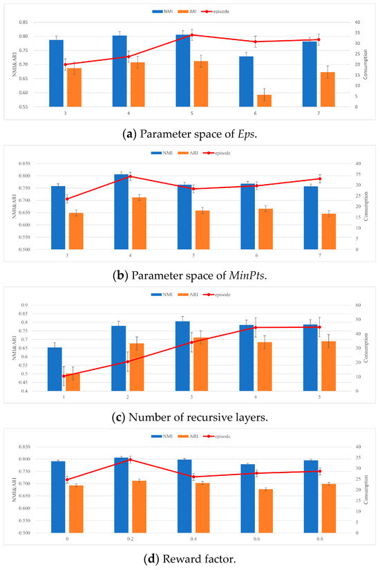
Figure 10. Effect of hyperparameter selection on the PER-SAC-based framework.

In addition to the above hyperparameters, the proportion occupied by labels used for model validation is 20%, and the dimensions of FCN (fully connected network) and MLP (multi-layer perceptron) are set to 32 and 256, respectively. The default values of other hyperparameters are shown in Table 6.

Table 6. Selection of hyperparameters.

Hyperparameters	Description	Default Values
$E_{max}$	Maximum number of rounds of training process	15
$B_{MinPts,2}^0$	Maximum search boundary for MinPts in Layer 0	0.25 × dataset size
$I_{max}$	Maximum search step in each round of episode	30
$\gamma$	Reward decay factor of Critic networks	0.1
$M$	Number of samples in the prioritized experience replay buffer	1

5.3.2. Comparison with Other Parameter Tuning Algorithms

We compare the proposed PER-SAC algorithm with K-Means [4], KANN [25], and the state-of-the-art DRL-based TD3 [31] and SAC [33] algorithms to evaluate the clustering accuracy of the optimal parameters obtained by these algorithms on DBSCAN. In the experiments, we use PER-SAC-DBSCAN to refer to the result that applies the optimal parameters obtained by the PER-SAC algorithm-based framework to the proposed STRP-DBSCAN algorithm. We evaluate all of the comparison algorithms by NMI and ARI values of clustering results on 3.3K and 8.5K labeled AIS datasets after preprocessing. Since DRL algorithms such as TD3 and SAC are somewhat randomized, we use the average values and standard deviations of NMI and ARI from ten runs of the algorithms to evaluate the clustering accuracy and stability, respectively. Table 7 shows the evaluation results with 3.3K and 3-classfied dataset.

Table 7. Evaluation results of parameter tuning algorithms with a 3.3K and 3-classfied dataset.

Item	K-Means [4]		KANN [25]		TD3-DBSCAN [31]		SAC-DBSCAN [33]		PER-SAC-DBSCAN
	NMI	ARI	NMI	ARI	NMI	ARI	NMI	ARI	NMI	ARI
1	0.6927	0.5242	0.6559	0.4994	0.776	0.678	0.8026	0.7005	0.8101	0.7174
2	0.6927	0.5242	0.6559	0.4994	0.76	0.6549	0.8087	0.7186	0.8114	0.7212
3	0.6927	0.5242	0.6559	0.4994	0.7632	0.6586	0.7935	0.6925	0.8114	0.7212
4	0.6927	0.5242	0.6559	0.4994	0.794	0.6963	0.8121	0.7209	0.8077	0.7179
5	0.6927	0.5242	0.6559	0.4994	0.7932	0.6955	0.8114	0.7212	0.8101	0.7174
6	0.6927	0.5242	0.6559	0.4994	0.8121	0.7209	0.7958	0.6995	0.8039	0.7018
7	0.6927	0.5242	0.6559	0.4994	0.78	0.6805	0.7698	0.6697	0.8117	0.7196
8	0.6927	0.5242	0.6559	0.4994	0.76	0.6549	0.8085	0.7136	0.8121	0.7209
9	0.6927	0.5242	0.6559	0.4994	0.8124	0.722	0.79	0.6925	0.7951	0.6937
10	0.6927	0.5242	0.6559	0.4994	0.7698	0.6697	0.7944	0.6969	0.7887	0.6876
AVG	0.6927	0.5242	0.6559	0.4994	0.782	0.6831	0.799	0.7026	0.806	0.7119
STD	-	-	-	-	0.019	0.024	0.012	0.015	0.008	0.012

As shown in Table 7, PER-SAC-DBSCAN improves the average NMI and ARI by 16.36% and 35.81% compared to K-Means, and by 22.88% and 42.55% compared to KANN. Compared to TD3-DBSCAN, PER-SAC-DBSCAN shows improvements of 3.07% and 4.22% in the average accuracy of NMI and ARI, and 137.50% and 100% in the stability of both metrics, respectively. Compared to SAC-DBSCAN, it improves the average accuracy of NMI and ARI by 0.88% and 1.32%, and improves the stability of both metrics by 50% and 25%, respectively.

We also evaluate the algorithms with an 8.5K and 5-classfied AIS dataset. Table 8 shows the evaluation results. PER-SAC-DBSCAN effectively improves the clustering accuracy of DBSCAN compared to K-Means and KANN by 12.84% and 5.03% in the average value of NMI, and by 12.07% and 12.97% in the average value of ARI, respectively. Compared to TD3-DBSCAN, PER-SAC-DBSCAN improves the average accuracy and stability of NMI by 1.19% and 85.71%, respectively. Although it has a slight loss by 1.13% in the average accuracy of ARI with TD3-DBSCAN, the stability of ARI is improved by 5.48%. Compared to SAC-DBSCAN, it improves the average accuracy of NMI and ARI by 1.68% and 0.07%, and the stability of both metrics by 57.14% and 1.37%, respectively.

Table 8. Evaluation results of parameter tuning algorithms with an 8.5K and 5-classfied dataset.

Item	K-Means [4]		KANN [25]		TD3-DBSCAN [31]		SAC-DBSCAN [33]		PER-SAC-DBSCAN
	NMI	ARI	NMI	ARI	NMI	ARI	NMI	ARI	NMI	ARI
1	0.7515	0.663	0.8074	0.6577	0.783	0.6438	0.8377	0.7464	0.835	0.7397
2	0.7515	0.663	0.8074	0.6577	0.8878	0.8344	0.8274	0.6623	0.8274	0.6673
3	0.7515	0.663	0.8074	0.6577	0.784	0.6463	0.8484	0.7617	0.8356	0.6697
4	0.7515	0.663	0.8074	0.6577	0.8346	0.7473	0.783	0.6438	0.835	0.7397
5	0.7515	0.663	0.8074	0.6577	0.8757	0.8188	0.8208	0.761	0.892	0.884
6	0.7515	0.663	0.8074	0.6577	0.8759	0.8212	0.8829	0.8324	0.8312	0.6658
7	0.7515	0.663	0.8074	0.6577	0.783	0.6438	0.8886	0.8828	0.8812	0.8267
8	0.7515	0.663	0.8074	0.6577	0.8634	0.8449	0.832	0.7358	0.8574	0.8051
9	0.7515	0.663	0.8074	0.6577	0.8439	0.7542	0.783	0.6438	0.8312	0.6658
10	0.7515	0.663	0.8074	0.6577	0.8474	0.7605	0.8375	0.7548	0.8518	0.7666
AVG	0.7515	0.663	0.8074	0.6577	0.838	0.7515	0.834	0.7425	0.848	0.743
STD	-	-	-	-	0.039	0.077	0.033	0.074	0.021	0.073

Based on the above results, it can be seen that the optimal parameters obtained by the PER-SAC algorithm-based autotuning framework can effectively improve the clustering accuracy and stability of DBSCAN on spatial-temporal trajectory data compared with the state-of-the-art algorithms. This is attributed to the fact that the combination of PER and SAC effectively improves the optimal-searching performance and the robustness of DRL. Moreover, the framework can autotune optimal parameters of DBSCAN with almost no human effort.

5.4. Overall Performance Comparison

In the previous experiments, datasets are preprocessed according to the methods described in Section 3.3 and Section 5.1 for the evaluation of algorithms. However, the proposed STRP-DBSCAN algorithm includes a preprocessing step for datasets, while other algorithms do not involve such steps. In this part, we use the original labeled 12K and 5-classified spatial-temporal trajectory dataset without preprocessing to evaluate the overall performance of STRP-DBSCAN with the PER-SAC-based parameter autotuning framework. The same dataset is also evaluated on KANN and TD3-DBSCAN in terms of clustering accuracy and execution time to conduct the comparison.

Table 9 shows the overall performance comparison results. Through the preprocessing step, STRP-DBSCAN screens and removes 28.8% of irregularities in the original dataset. Therefore, compared with other two algorithms, the proposed STRP-DBSCAN with PER-SAC has further optimized the clustering accuracy and clustering time on the original trajectory dataset. According to Table 9, the proposed STRP-DBSCAN with PER-SAC improves the accuracy of NMI and ARI by 14.03% and 39.80% compared to KANN, and by 3.71% and 8.82% compared to TD3-DBSCAN, respectively. Since KANN adopts a cyclic iterative optimization strategy for parameter searching, it takes a very long time to find the optimal parameters of DBSCAN, which costs about 10 h in the experiments and is completely uncompetitive. Compared with TD3-DBSCAN, STRP-DBSCAN with PER-SAC improves the clustering efficiency by 25.60% in term of the total execution time of the algorithms.

Table 9. Overall performance comparison with the original labeled 12K and 5-classified AIS dataset.

Item	STRP-DBSCAN + PER-SAC	KANN [25]	TD3-DBSCAN [31]
NMI	0.9207	0.8074	0.8878
ARI	0.9194	0.6577	0.8449
Total execution time	342.05 s	About 10 h	429.6 s

Figure 11 shows the visualization results of the clustering effect of the evaluated algorithms, which is more intuitive. It can be seen that the clustering result of the proposed STRP-DBSCAN with PER-SAC is significantly better than KANN. It also outperforms TD3-DBSCAN in terms of clustering accuracy.

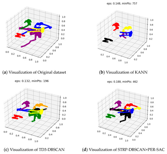
Figure 11. Visualization results of different clustering algorithms with the 12K and 5-classified AIS dataset.

6. Conclusions

In this paper, the parallel DBSCAN algorithm for spatial-temporal trajectory data is revisited. A STRP-DBSCAN algorithm based on spatial-temporal random partitioning is proposed. The algorithm reduces the noise points in the original dataset through data preprocessing and introduces the idea of temporal partitioning on the basis of the state-of-the-art RP-DBSCAN algorithm, which divides the data points into more balanced partitions in both spatial and temporal attributes. Therefore, it further enhances the execution efficiency of the parallel DBSCAN algorithm to a certain extent. In addition, the PER-SAC algorithm is proposed, which combines the prioritized experience replay mechanism and SAC algorithm to search the optimal clustering parameter. Based on PER-SAC, an optimal parameter autotuning framework is realized to efficiently autotune the optimal DBSCAN clustering parameters, which improves the clustering accuracy of the spatial-temporal trajectory data. The experimental results show that the proposed algorithm outperforms state-of-the-art DBSCAN algorithms in both clustering time and clustering accuracy, reducing the clustering time by up to 31.2% and improving the clustering accuracy by up to 8.8% on the tested AIS datasets. And it achieves more stable clustering results. Since the proposed PER-SAC algorithm uses NMI as the reward metric, it is currently only applicable to labeled datasets. Our future work will investigate the parameter autotuning method for unlabeled data to improve the generalizability of this work.

References

- Dokuz, A.S. Weighted spatio-temporal taxi trajectory big data mining for regional traffic estimation. Phys. A 2022, 589, 126645. [Google Scholar] [CrossRef]
- Yang, J.; Liu, Y.; Ma, L.; Ji, C. Maritime traffic flow clustering analysis by density based trajectory clustering with noise. Ocean Eng. 2022, 249, 111001. [Google Scholar] [CrossRef]
- Wojciechowski, T.W.; Sadler, R.C.; Buchalski, Z.; Harris, A.; Lederer, D.; Furr-Holden, C.D. Trajectory Modeling of Spatio-Temporal Trends in COVID-19 Incidence in Flint and Genesee County, Michigan. Ann. Epidemiol. 2022, 67, 29–34. [Google Scholar] [CrossRef]
- Likas, A.; Vlassis, N.; Verbeek, J.J. The global k-means clustering algorithm. Pattern Recognit. 2003, 36, 451–461. [Google Scholar] [CrossRef]
- Ester, M.; Kriegel, H.P.; Sander, J.; Xu, X. A density-based algorithm for discovering clusters in large spatial databases with noise. In Proceedings of the KDD-96 Proceedings, Oregon, Portland, 2–4 August 1996. [Google Scholar]
- Huang, M.; Bao, Q.; Zhang, Y.; Feng, W. A hybrid algorithm for forecasting financial time series data based on DBSCAN and SVR. Information 2019, 10, 103. [Google Scholar] [CrossRef]
- Fan, T.; Guo, N.; Ren, Y. Consumer clusters detection with geo-tagged social network data using DBSCAN algorithm: A case study of the Pearl River Delta in China. Geol. J. 2021, 86, 317–337. [Google Scholar] [CrossRef]
- Birant, D.; Kut, A. ST-DBSCAN: An algorithm for clustering spatial–temporal data. Data Knowl. Eng. 2007, 60, 208–221. [Google Scholar] [CrossRef]
- Wang, C.; Li, J.; He, Y.; Xiao, K.; Hu, C. Segmented trajectory clustering-based destination prediction in IoVs. IEEE Access 2020, 8, 98999–99009. [Google Scholar] [CrossRef]
- Song, H.; Lee, J.-G. RP-DBSCAN: A superfast parallel DBSCAN algorithm based on random partitioning. In Proceedings of the 2018 International Conference on Management of Data, Houston, TX, USA, 10–15 June 2018. [Google Scholar]
- Rdusseeun, L.; Kaufman, P. Clustering by means of medoids. In Proceedings of the Statistical Data Analysis Based on the L1 Norm Conference, Neuchatel, Switzerland, 31 August–4 September 1987. [Google Scholar]
- Zhang, T.; Ramakrishnan, R.; Livny, M. BIRCH: A new data clustering algorithm and its applications. Data Min. Knowl. Discov. 1997, 1, 141–182. [Google Scholar] [CrossRef]
- Guha, S.; Rastogi, R.; Shim, K. CURE: An efficient clustering algorithm for large databases. ACM Sigmod Rec. 1998, 27, 73–84. [Google Scholar] [CrossRef]
- Wang, W.; Yang, J.; Muntz, R. STING: A statistical information grid approach to spatial data mining. In Proceedings of the VLDB, Athens, Greece, 26–29 August 1997. [Google Scholar]
- Agrawal, R.; Gehrke, J.; Gunopulos, D.; Raghavan, P. Automatic subspace clustering of high dimensional data for data mining applications. In Proceedings of the 1998 ACM SIGMOD international conference on Management of data, Seattle, DC, USA, 2–4 June 1998. [Google Scholar]
- Fraley, C.; Raftery, A.E. Model-based clustering, discriminant analysis, and density estimation. J. Am. Stat. Assoc. 2002, 97, 611–631. [Google Scholar] [CrossRef]
- Crespo, R.; Alvarez, C.; Hernandez, I.; García, C. A spatially explicit analysis of chronic diseases in small areas: A case study of diabetes in Santiago, Chile. Int. J. Health Geogr. 2020, 19, 1–13. [Google Scholar] [CrossRef]
- Ankerst, M.; Breunig, M.M.; Kriegel, H.-P.; Sander, J. OPTICS: Ordering points to identify the clustering structure. ACM Sigmod Rec. 1999, 28, 49–60. [Google Scholar] [CrossRef]
- Garyfallidis, E.; Brett, M.; Correia, M.M.; Williams, G.B.; Nimmo-Smith, I. Quickbundles, a method for tractography simplification. Front. Neurosci. 2012, 6, 175. [Google Scholar] [CrossRef]
- Choi, C.; Hong, S.-Y. Mdst-dbscan: A density-based clustering method for multidimensional spatiotemporal data. ISPRS Int. J. Geo-Inf. 2021, 10, 391. [Google Scholar] [CrossRef]
- Xu, X.; Jäger, J.; Kriegel, H.-P. A fast parallel clustering algorithm for large spatial databases. In High Performance Data Mining: Scaling Algorithms, Applications and Systems; Springer: Boston, MA, USA, 2002; pp. 263–290. [Google Scholar]
- Prokopenko, A.; Lebrun-Grandie, D.; Arndt, D. Fast tree-based algorithms for DBSCAN for low-dimensional data on GPUs. In Proceedings of the ICPP 2023, Salt Lake City, UT, USA, 7–10 August 2023. [Google Scholar]
- Hou, J.; Gao, H.; Li, X. DSets-DBSCAN: A parameter-free clustering algorithm. IEEE Trans. Image Process. 2016, 25, 3182–3193. [Google Scholar] [CrossRef] [PubMed]
- Kim, J.-H.; Choi, J.-H.; Yoo, K.-H.; Nasridinov, A. AA-DBSCAN: An approximate adaptive DBSCAN for finding clusters with varying densities. J. Supercomput. 2019, 75, 142–169. [Google Scholar] [CrossRef]
- Li, W.J.; Yan, S.Q.; Jiang, Y.; Zhang, S.; Wang, C. Algorithmic research on adaptive determination of DBSCAN algorithm parameters. Comput. Appl. Eng. Educ. 2019, 55, 1–7. [Google Scholar]
- Falahiazar, Z.; Bagheri, A.; Reshadi, M. Determining the Parameters of DBSCAN Automatically Using the Multi-Objective Genetic Algorithm. J. Inf. Sci. Eng. 2021, 37, 157–183. [Google Scholar]
- Li, Y. Deep reinforcement learning: An overview. arXiv 2017, arXiv:1701.07274. [Google Scholar] [CrossRef]
- LeCun, Y.; Bengio, Y.; Hinton, G. Deep learning. Nature 2015, 521, 436–444. [Google Scholar] [CrossRef] [PubMed]
- Sutton, R.S.; Barto, A.G. Reinforcement Learning: An Introduction; MIT Press: Cambridge, MA, USA, 2018. [Google Scholar]
- Peng, H.; Zhang, R.; Li, S.; Cao, Y.; Pan, S.; Philip, S.Y. Reinforced, incremental and cross-lingual event detection from social messages. IEEE Trans. Pattern Anal. Mach. Intell. 2022, 45, 980–998. [Google Scholar] [CrossRef] [PubMed]
- Zhang, R.; Peng, H.; Dou, Y.; Wu, J.; Sun, Q.; Li, Y.; Zhang, J.; Yu, P.S. Automating DBSCAN via deep reinforcement learning. In Proceedings of the CIKM 2022, Atlanta, GA, USA, 16 October 2022. [Google Scholar]
- Fujimoto, S.; Hoof, H.; Meger, D. Addressing function approximation error in actor-critic methods. In Proceedings of the ICML 2018, Stockholmsmässan, Stockholm, Sweden, 10–15 July 2018. [Google Scholar]
- Haarnoja, T.; Zhou, A.; Hartikainen, K.; Tucker, G.; Ha, S.; Tan, J.; Kumar, V.; Zhu, H.; Gupta, A.; Abbeel, P. Soft actor-critic algorithms and applications. arXiv 2018, arXiv:1812.05905. [Google Scholar]
- Mnih, V.; Kavukcuoglu, K.; Silver, D.; Graves, A.; Antonoglou, I.; Wierstra, D.; Riedmiller, M. Playing atari with deep reinforcement learning. arXiv 2013, arXiv:1312.5602. [Google Scholar]
- Schaul, T.; Quan, J.; Antonoglou, I.; Silver, D. Prioritized experience replay. arXiv 2015, arXiv:1511.05952. [Google Scholar]
- China Offshore AIS Open Source Data. 2022. Available online: https://www.heywhale.com/mw/dataset/623b00c9ae5cf10017b18cc6/content (accessed on 16 March 2023).
- Rousseeuw, P.J. Silhouettes: A graphical aid to the interpretation and validation of cluster analysis. J. Comput. Appl. Math. 1987, 20, 53–65. [Google Scholar] [CrossRef]
- Davies, D.L.; Bouldin, D.W. A cluster separation measure. IEEE Trans. Pattern Anal. Mach. Intell. 1979, 2, 224–227. [Google Scholar] [CrossRef]
- Estévez, P.A.; Tesmer, M.; Perez, C.A.; Zurada, J.M. Normalized mutual information feature selection. IEEE Trans. Neural Netw. 2009, 20, 189–201. [Google Scholar] [CrossRef]
- Vinh, N.X.; Epps, J.; Bailey, J. Information theoretic measures for clusterings comparison: Is a correction for chance necessary? In Proceedings of the ICML 2009, Montreal, Canada, 14–18 June 2009. [Google Scholar]
- Kanervisto, A.; Scheller, C.; Hautamäki, V. Action space shaping in deep reinforcement learning. In Proceedings of the CoG 2020, Osaka, Japan, 24–27 August 2020. [Google Scholar]
Disclaimer/Publisher’s Note: The statements, opinions and data contained in all publications are solely those of the individual author(s) and contributor(s) and not of MDPI and/or the editor(s). MDPI and/or the editor(s) disclaim responsibility for any injury to people or property resulting from any ideas, methods, instructions or products referred to in the content. |
© 2023 by the authors. Licensee MDPI, Basel, Switzerland. This article is an open access article distributed under the terms and conditions of the Creative Commons Attribution (CC BY) license (https://creativecommons.org/licenses/by/4.0/).