Prediction of Gasoline Orders at Gas Stations in South Korea Using VAE-Based Machine Learning Model to Address Data Asymmetry

Abstract

South Korea has developed road-based transportation and uses a lot of gasoline. South Korea imports gasoline since it is not produced domestically. So, fluctuations in gasoline prices have a significant impact on the national economy. Currently, gasoline orders, which are based on gasoline consumption, are analyzed in relation to fluctuations in gasoline prices. However, gasoline orders can also change due to various non-price factors. Therefore, to understand the trend of gasoline orders, it is important to identify additional factors that gas stations consider when determining orders. We collected 180 monthly samples of data on 167 variables. Sudden international issues lead to rapid fluctuations in gasoline orders, which can lead to outliers. A class imbalance occurs because outliers are generally fewer in number than the normal data points. Therefore, to address the class imbalance, we proposed a method that grouped the data samples into 11 clusters using the K-means clustering algorithm and then augmented the data into 85 datasets in each cluster through the Variational Auto-Encoder. We evaluated the augmented datasets through the R-Squared, Root Mean Squared Errors, and accuracy of various regression models. Based on the experimental results, when predicting gasoline orders at gas stations in South Korea using augmented datasets, linear regression showed the best performance.

1. Introduction

South Korea is the seventh largest energy consumer in the world [1]. However, lacking domestic resources, the country relies on imports to meet its consumption needs. Crude oil, which accounts for a significant portion of energy consumption, is not produced domestically, so 98% of its demand is imported. Therefore, changes in international crude oil prices have a significant impact on South Korea’s national economy.

The domestic transportation sector is particularly dependent on crude oil [2]. According to the Ministry of Trade, Industry, and Energy, petroleum products processed from crude oil accounted for 95.12% of the energy consumption in the domestic transportation sector in December 2022 [3]. Since South Korea’s transportation system is road-based, the trend of energy consumption in the domestic transportation sector is analyzed based on the consumption of diesel and gasoline as representative fuels. In particular, the price of gasoline is sensitive to changes, and its consumption causes large fluctuations in price. In South Korea, gasoline order fluctuations underlie gasoline consumption patterns.

Recently, empirical studies have studied the flow of gasoline orders through the correlation between international crude oil prices and gasoline prices [4,5,6,7,8]. Bacon [4] found that gasoline prices rise rapidly when international crude oil prices increase but decline slowly when international crude oil prices decrease. Gasoline prices reflect changes in international crude oil prices but not in a balanced or symmetrical way. This means that international crude oil prices and gasoline prices change asymmetrically. This price asymmetry between international crude oil and gasoline has been likened to the “rockets and feathers” phenomenon. Borenstein et al. [5] analyzed the impact of gasoline supply adjustments due to the international crude oil shock on wholesale and retail gasoline prices. The costs with supply adjustments included stickiness and asymmetry in gasoline prices. Kim [6] analyzed the asymmetry in gasoline price adjustments and international crude oil prices using four datasets: the weekly Dubai crude oil price, gasoline prices at refineries, gasoline prices at gas stations, and exchange rates. Price asymmetry arose due to the cost of managing the gasoline at refineries and gas stations. Kim et al. [7] analyzed the asymmetry of gasoline price adjustments due to changes in international crude oil prices based on changes within three months using the daily gasoline price and Dubai crude oil price. They found that the volatility in international crude oil prices amplified the asymmetry in gasoline prices. In contrast, the government’s policy to cut fuel taxes weakened the asymmetry. Bae et al. [8] analyzed the asymmetry of US Gulf gasoline prices and West Texas Intermediate (WTI) crude oil. The entire analysis period was divided into five intervals associated with periods of stable international oil prices, increasing international oil prices, and global economic crises. It was found that the degree of asymmetry in gasoline prices was influenced by the global economy.

Gasoline prices are closely related to fluctuations in international crude oil prices and gasoline orders, and they become more sensitive when crude oil prices rise. However, gasoline orders can also change due to various non-price factors. According to an analysis of national energy supply and demand trends, the monthly average international gasoline (95 Research Octane Number, 95RON) price of the Mean of Platt’s Singapore Kerosene (MoPS) fell by KRW 26.19 in November 2021 [9]. Additionally, since 12 November 2021, the fuel tax imposed on gasoline has decreased by 20%. However, gasoline orders increased by only 2.74% compared to the previous month, and the retail price of gasoline at gas stations rose by KRW 25 per liter. This phenomenon means that non-price factors have a significant impact on gasoline orders, given the COVID-19 pandemic, the continued rise in international crude oil prices, and the global economic downturn. Consequently, to understand the trend of gasoline consumption in the transportation sector, it is important to identify additional factors, other than price, that gas stations consider when determining orders.

To analyze and predict the factors that determine gasoline orders at gas stations, monthly data related to the prices of crude oil and gasoline, economy, stocks, climate, environment, and policy from January 2008 to December 2022 were collected. As gasoline orders are collected monthly in accordance with the Domestic Petroleum and Alternative Fuel Business Act [10], there was a limitation in that only 180 months of data samples could be used. Outliers in small amounts of data samples risk degrading the performance of models. Sudden international issues, such as disputes, wars, and infectious diseases, lead to rapid fluctuations in gasoline orders, which can lead to outliers. However, to better understand gasoline orders, considering outliers is essential. A class imbalance occurs because outliers are generally fewer in number than normal data points. Therefore, it is necessary to augment data samples while considering their characteristics to address the class imbalance. By resolving the class imbalance in data samples, models with more stable performance can be developed. We proposed a method to group data samples into clusters using the K-means clustering algorithm [11] and then augment the datasets in the cluster through the Variational Auto-Encoder (VAE) [12]. The augmented datasets were used in our proposed linear regression model to identify the fluctuation factors in gasoline orders at gas stations.

The main contributions are summarized as follows:

• We proposed a gasoline order prediction model for gas stations using a linear regression model to understand the trend of gasoline consumption in South Korea.
• We proposed a Variational Auto-Encoder (VAE) and K-means clustering algorithm to address data asymmetry.

  ○

  We performed data augmentation on our model with the Variational Auto-Encoder (VAE) to implement a model with high accuracy and generalized performance.

  ○

  We grouped the datasets into clusters using the K-means clustering and then augmented each cluster’s datasets with VAE to better reflect the characteristics of the data samples for augmentation.

• We found significant independent variables that influence gasoline orders using the Variance Inflation Factor (VIF) and p-value.
• We confirmed that linear regression is the most suitable method for the prediction of gasoline orders through modeling with various regression models.

The structure of this paper is as follows: Section 2 describes related works. Section 3 describes a gasoline order prediction model using augmented datasets. Section 4 shows the results. Section 5 presents the discussions and conclusions.

2. Related Works

We proposed K-means clustering with the elbow method [11,13,14] to group the data samples into 11 clusters. In each cluster, we augmented the data samples using a Variational Auto-Encoder (VAE) [12,15,16] to resolve the class imbalance in the data samples. The augmented data samples were used to predict gasoline orders with regression models [17,18,19,20,21,22,23].

2.1. K-Means Clustering

Clustering is an effective algorithm for searching data samples and grouping similar types [11]. It is an unsupervised learning algorithm in machine learning that automatically identifies characteristics and patterns within given datasets and groups based on their similarities. Among them, K-means clustering is a distance-based clustering algorithm that randomly specifies centroids and groups the datasets into $K$ clusters. The clusters are optimized by iteratively moving the centroid to find a location where the distance between the datasets and the centroid in the generated cluster is minimized. The actual number of clusters in the datasets is determined using the elbow method [11,13,14]. This involves calculating the change in the distance between centroids and datasets by adjusting the number of clusters. The point where the distance drops dramatically and then reaches the plateau is called the “elbow”, and the cluster $K$ corresponding to the elbow’s point is the optimal value. Gharibi et al. [13] used the elbow method to optimize the number of clusters in the K-means clustering algorithm. Charging scheduling data samples of electric vehicles were grouped into four clusters. Omar et al. [14] used the elbow method to group data samples into the optimal number of clusters. Health insurance premium data samples were grouped into three clusters. Using K-means clustering with the elbow method, data samples with various characteristics can be grouped into the optimal cluster.

2.2. Variational Auto-Encoder

The Variational Auto-Encoder (VAE) is a generative model that models the distribution of given datasets and generates new datasets [12,15,16]. VAE is used when the amount of data is sparse and is useful for augmenting datasets while preserving the distribution of their features. It uses a stochastic approach to learn latent variables to express the different features and variability of datasets. VAE consists of two layers: an encoder and a decoder. The encoder layer generates a low-dimensional latent variable from the input datasets. The decoder layer constructs a Gaussian probability distribution based on the mean and variance of the latent variable and restores the datasets based on features randomly acquired from the probability distribution. The reconstruction error and Kullback–Leibler (KL) divergence are employed as cost functions to evaluate the reconstruction performance of the decoder layer. The datasets generated through the decoder layer are similar to the input datasets but have non-linear lower dimensions. Maity et al. [15] augmented outliers using VAE to detect Alzheimer’s disease in brain MRI data samples. The Alzheimer’s patient data samples were augmented to match the class ratio of healthy brain datasets. Kim et al. [16] augmented outliers using VAE to detect lifelog anomalies collected through wearable devices. The anomaly data samples were augmented to solve the class imbalance. VAE can help address class imbalances in data samples.

2.3. Regression

Regression is an effective machine learning algorithm for predicting future outcomes based on past data. Linear regression is a type of regression used to discover the linear correlation between a dependent variable and one or more independent variables and to predict the value of the dependent variable for new independent variables. The linear regression model is defined as in Equation (1):

$$y=w_1{x}_1+w_2{x}_2+\cdots +w_n{x}_n$$

(1)

where $y$ is the dependent variable, and $x_1$, $x_2$, $\cdots$, $x_n$ are the independent variables. $w_1$, $w_2$, $\cdots$, $w_n$ are the weights of each independent variable. The linear regression model finds the best-fitting linear relationship between the dependent and independent variables by learning the most suitable weights.

Overfitting can occur in a high-dimensional linear regression model with a large number of independent variables. Accordingly, the Lasso [17], Ridge [18], and Elastic-Net [19] regression methods, which reduce the complexity of the linear regression model by adding a regularization term to it, were developed. These three models commonly decrease the weight of each independent variable through regularization terms. The regularization term of the Lasso regression is based on L1 normalization (Manhattan distance and Taxicab geometry). The regularization term of the Ridge regression is based on L2 normalization (Euclidean distance). Elastic-Net regression utilizes both L1 and L2 normalization-based regularization terms and finds the optimal value by adjusting the usage ratio of each term. However, when dealing with a linear regression model with fewer independent variables, introducing a regularization term can heavily influence the model, potentially leading to underfitting.

2.4. Ensemble

Ensemble is a machine learning algorithm that combines multiple decision tree models to create a more robust and accurate predictive model. There are four representative models: the Random Forest regression, Extra Trees regression, AdaBoost regression, and XGBoost regression. The Random Forest regression randomly selects independent variables to create decision trees and outputs average predictions from multiple trees [20]. The Extra Trees regression adds more randomness than the Random Forest regression by randomly selecting subsets of data samples to create decision trees [21]. The AdaBoost regression iteratively focuses on outliers during training [22]. The XGBoost (Extreme Gradient Boosting) regression assigns weights to each independent variable to create decision trees and enhances the model using gradient information from residual errors [23]. Since ensemble models are composed of combinations of multiple trees, there are limitations in comprehending the importance of individual independent variables. In addition, modeling with linear datasets can lead to similar predictions from individual trees, limiting the performance of ensemble models. Some ensembles are modeled for classification and may not be suitable for regression models.

3. Material and Methods

Previous studies [4,5,6,7,8] have analyzed gasoline order patterns in the relationship between international crude oil and gasoline prices. However, changes in gasoline orders are influenced not only by gasoline prices but also by external factors. Therefore, we propose a gasoline order prediction model using data such as the prices of crude oil and gasoline, the economy, stocks, the climate, the environment, and policy. To construct a model that fully considers the outliers caused by rapid fluctuations in gasoline orders due to diverse causes, we first grouped the data into $K$ clusters with the K-means clustering algorithm. Then, we solved the data imbalance and shortage issues using VAE. The augmented data were used to build linear regression and to discover the important fluctuation factors in gasoline orders. Using the proposed method, we were able to discover the importance of each fluctuation factor.

Figure 1 shows a flow diagram of our proposed method: data collection, data augmentation with K-means clustering and VAE, data preprocessing, modeling, and evaluations.

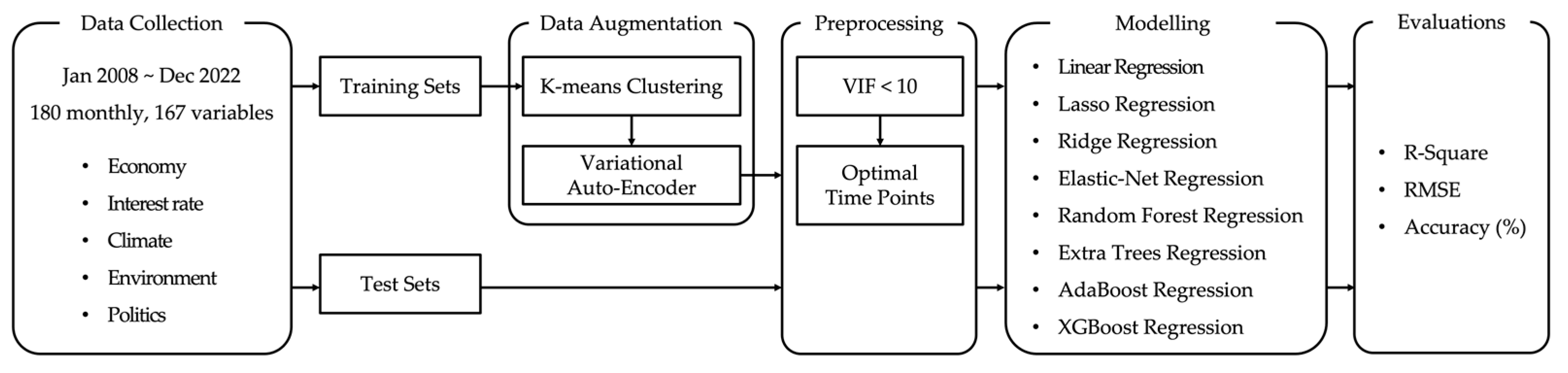
3.1. Data Collection

To predict gasoline orders at gas stations in South Korea, we used 167 variables for the prices of crude oil and gasoline, the economy, stocks, the climate, the environment, and policy from January 2008 to December 2022. All 167 collected variables contained 180 monthly data samples, without missing values. The crude oil price and gasoline price data were collected from Korea National Oil Corporation’s oil price information service (Opinet) [24]. Opinet collects international gasoline (95RON) prices from Mean of Platt’s Singapore Kerosene (MoPS). Economy-related datasets were obtained from the Economic Statistics System (ECOS) [25]. Stock-related datasets were collected from Investing.com. Climate- and environment-related datasets were retrieved from the Korea Meteorological Administration [26]. The government policy and gas station management datasets were obtained from Petronet [27]. All data collection sources are reliable.

3.2. Data Augmentation with Variational Auto-Encoder

COVID-19, the oil price war, crude oil reduction, and terrorism have caused a significant change in the global economy. These factors have also had a huge impact on the fluctuation in gasoline orders at gas stations. Governments typically cut fuel taxes to resolve the issues caused by huge fluctuations in gasoline oil prices. This policy of cutting fuel taxes also affects the fluctuations in gasoline orders. Since these factors are temporary phenomena that occur at certain points in time, they can be called “outliers” in relation to all the data samples. Outliers are fewer in number than the normal data points, resulting in a class imbalance. To accurately understand gasoline orders, it is necessary to construct a model with sufficient consideration of outliers.

To compensate for the class imbalance, the datasets were grouped into clusters with the K-means clustering algorithm and then augmented with VAE for each cluster. Figure 2 shows a flowchart of the data augmentation process.

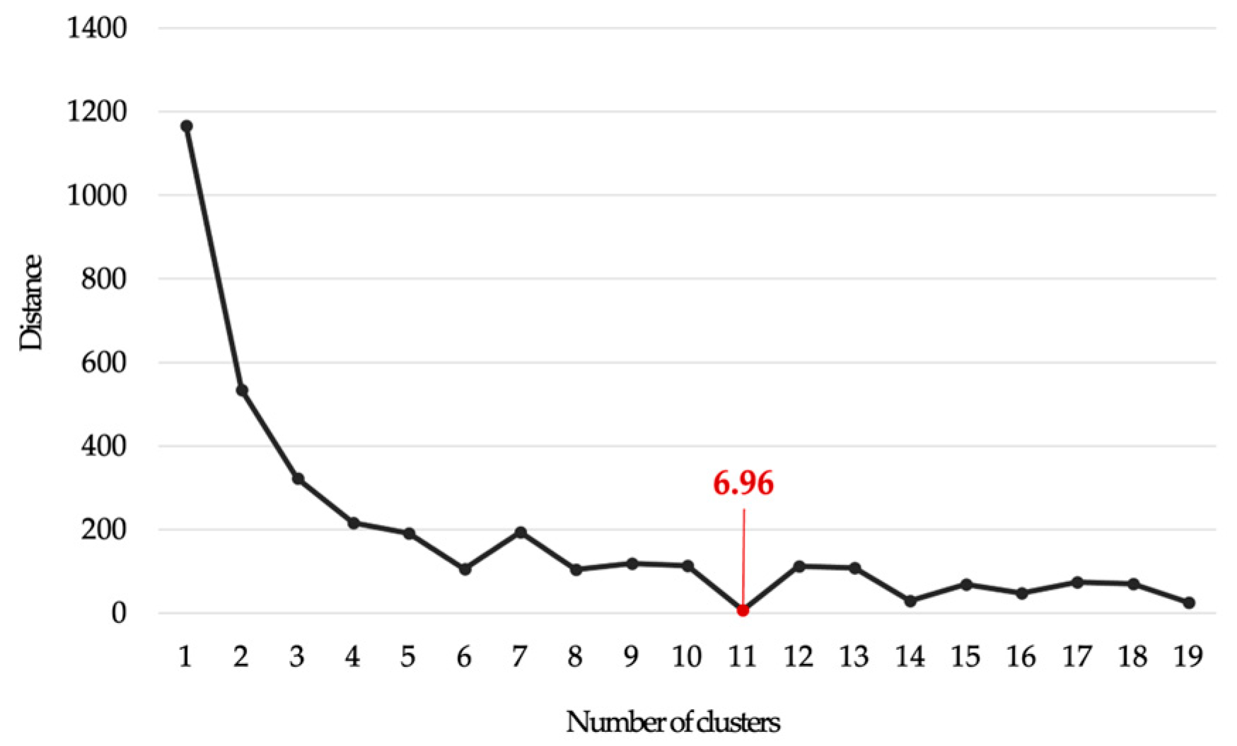
• First, we grouped the training data into $K$ clusters. $K$ was set to 11, which was decided using the elbow method of the K-means clustering algorithm (refer to Section 2.1). The elbow method shows that the data have been organized using a visual analysis and gives insight into the optimal value of $K$.
• Figure 3 shows the changes in the similarity distance according to the number ($K$) of clusters. When $K$ was set to 11, the distance dramatically decreased. The separate $K$ clusters consisted of 4 to 28 datasets. However, to obtain a good performance of the machine learning algorithm, it is best if the amount of data in each cluster is similar.
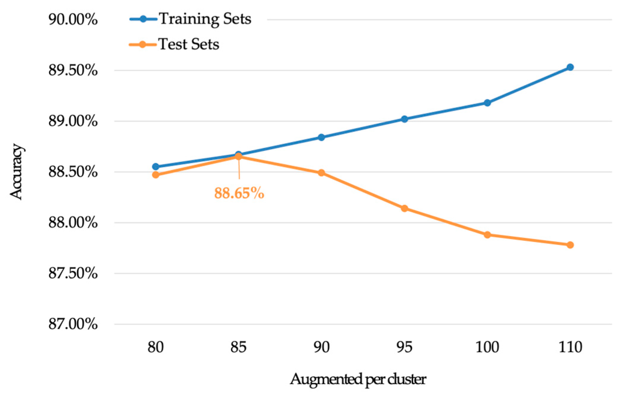
• The amount of data in each cluster should therefore be evenly distributed. To meet this objective, the data in each group were standardized. The standardized data were augmented with VAE. The data within each cluster were augmented to 85 sets, and the total number of augmented training sets was 935.

3.3. Preprocessing and Exploration of Independent Variables

With 167 variables from the augmented data, we evaluated multicollinearity using the Variance Inflation Factor (VIF) and searched for significant variables. VIF is a measure used to avoid collisions and duplications between variables and to increase model reliability by identifying correlations between the predictors in regression. Variables with a VIF of less than 10 were considered as significant variables [28,29,30]. Among the total of 167 variables, 11 significant variables were derived by repeatedly removing the variable with the highest VIF. The VIFs of the significant independent variables in the gasoline order prediction model are presented in

Table 1. Significant independent variables derived from VIF.

Category	Variables	VIF
Climate	Cooling degree day	1.1
Prices	Dubai crude oil prices	8.7
	International gasoline (95RON) prices	8.8
Stocks	FFR	1.4
	USDX	4.4
	S&P 500	4.0
Economy	PPI fluctuation rate	1.8
	NSI	2.1
Policy	GPR	1.8
	Fuel tax	1.7
Management	Gasoline inventory at the gas station	1.2

.

Furthermore, the optimal time points for the impact of each independent variable on gasoline orders are needed.

Table 2. The optimal time points for impact of each variable from VIF, used as independent variables for predicting gasoline orders at gas stations in South Korea.

Category	Variables	Point
Climate	Cooling degree day	$t-12$
Prices	Dubai crude oil prices	$t-3$
	International gasoline (95RON) prices	$t-1$
Stocks	FFR	$t-2$
	USDX	$t-1$
	S&P 500	$t$
Economy	PPI fluctuation rate	$t-2$
	NSI	$t-1$
Policy	GPR	$t-1$
	Fuel tax	$t$
Management	Gasoline inventory at the gas station	$t-1$

$t$ is monthly from January 2008 to December 2022.

describes the overall variables in the gasoline order prediction model. The independent variables related to gasoline orders for a particular month $t$ are as follows: the cooling degree day ($t-12$), Dubai crude oil prices ($t-3$), Federal Funds Rate (FFR) ($t-2$), US Producer Price Index (PPI) fluctuation rate ($t-2$), News Sentiment Index (NSI) ($t-1$), US Dollar Index (USDX) ($t-1$), international gasoline (95RON) prices ($t-1$), Geopolitical Risk Index (GPR) ($t-1$), gasoline inventory at the gas station ($t-1$), Standard & Poor’s 500 stock (S&P 500) ($t$), and fuel tax ($t$).

3.4. Modeling

In this study, K-means clustering was used to group 11 clusters according to the characteristics of the data, and each cluster was augmented to 85 data samples using VAE to solve the class imbalance problem (refer to Section 3.2).

To determine the significance of utilizing data samples that solved the class imbalance problem and the optimal number of augmentations, linear regression was used to analyze the change in performance according to the number of augmentations and method of augmentation (refer to

Table 3. Quantitative evaluation of linear regression for gasoline orders at gas stations in South Korea.

	Augmented per Cluster	Number of Training Sets	R-Squared		RMSE		Accuracy
			Training Sets	Test Sets	Training Sets	Test Sets	Training Sets	Test Sets
Without Augmentation	-	144	0.7441	0.7162	0.4898	0.5827	86.26%	84.63%
VAE	-	935	0.7490	0.7204	0.1931	0.5598	86.54%	84.88%
K-means Clustering + VAE	80	880	0.7842	0.7827	0.2666	0.4359	88.55%	88.47%
	85	935	0.7862	0.7858	0.2614	0.4328	88.67%	88.65%
	90	990	0.7892	0.7831	0.2569	0.4355	88.84%	88.49%
	95	1045	0.7924	0.7759	0.2513	0.4416	89.02%	88.14%
	100	1100	0.7953	0.7722	0.2464	0.4463	89.18%	87.88%
	110	1210	0.8016	0.7706	0.2381	0.4479	89.53%	87.78%

). The changes in performance based on regularization terms were compared and analyzed using linear regression, Lasso regression, Ridge regression, and Elastic-Net regression. We also evaluated the performance with ensemble models, such as AdaBoost regression, Extra Trees regression, Random Forest regression, and XGBoost regression.

4. Experimental Results

We implemented our proposed method in Python 3.9, Jupyter notebook platform, and PyTorch framework. We used a MacBook Air with an Apple M2 silicon chip 8-core CPU, 10-core GPU, 16 GB memory, 512 GB storage, and MacOS Ventura.

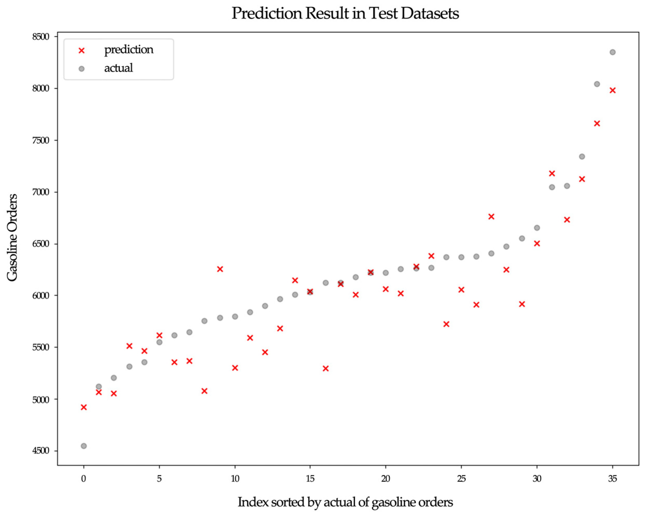
4.1. Evaluation of the Prediction of Gasoline Orders Using Data Augmentation

A total of 180 monthly data samples from January 2008 to December 2022 were randomly split into 80% training sets and 20% test sets. This ratio is commonly used in many previous studies [31,32,33]. In addition, Ref. [34] demonstrated that optimal results can be obtained when using 80% training sets and 20% test sets. To validate the impact of data augmentation, we quantitatively evaluated gasoline order prediction models using three methods: without augmentation, with VAE, and with K-means clustering and VAE together. The models were evaluated by using R-Squared, Root Mean Squared Errors (RMSE), and accuracy. The details of the equations of R-Squared, RMSE, and accuracy are described in Equation (A1) in Appendix A. R-Squared indicates how well the model explains the variability of given datasets. RMSE evaluates the performance of the model by measuring the difference between the actual and predicted values. Accuracy indicates how well the predictions in the model match the actual values. R-Squared and RMSE have values between 0 and 1. Accuracy has a percentage between 0 and 100. A higher R-Squared and accuracy, and a lower RMSE indicate a better performing model. When R-Squared is close to 1, accuracy is close to 100%, and RMSE is close to 0, the model is more successful. Table 3 shows the results. The performance was lower in all evaluation metrics when the datasets were not augmented. When the datasets were augmented using VAE, the accuracy of the test sets improved by 0.25%p compared to that of the non-augmented datasets. However, the significant difference in RMSE between the training and test sets indicates overfitting. Using the K-means clustering algorithm to group clusters and subsequently augmenting the datasets within each cluster resulted in a better representation of the data characteristics, leading to improved generalization performance and accuracy of the model. When the number of datasets per cluster was augmented to 85, the highest performance was shown in all evaluations of the test sets. Figure 4 shows the change in accuracy based on the number of augmented datasets per cluster.

4.2. Evaluation of the Prediction of Gasoline Orders Using Regression Models

Our proposed regression models used 935 augmented datasets. The datasets were grouped into 11 clusters using the K-means clustering algorithm, and then 85 datasets within each cluster were obtained using VAE.

Table 4. Quantitative evaluation of prediction models for gasoline orders using regularization terms for linear regression.

Regression Models	Regularization		R-Squared		RMSE		Accuracy
	Weight	L1:L2	Training Sets	Test Sets	Training Sets	Test Sets	Training Sets	Test Sets
Linear	-	-	0.7862	0.7858	0.2614	0.4328	88.67%	88.65%
Ridge	0.01	-	0.7862	0.7810	0.2613	0.4376	88.66%	88.37%
	0.1	-	0.7849	0.7816	0.2622	0.4370	88.60%	88.40%
	1	-	0.7885	0.7834	0.2602	0.4352	88.80%	88.51%
	10	-	0.7873	0.7827	0.2611	0.4359	88.73%	88.47%
Lasso	0.01	-	0.7764	0.7756	0.2673	0.4429	88.11%	88.07%
	0.1	-	0.6962	0.6851	0.3117	0.5247	83.44%	82.77%
	1	-	0.0000	−0.0525	0.5665	0.9593	00.00%	00.00%
	10	-	0.0000	−0.0515	0.5637	0.9588	00.00%	00.00%
Elastic-Net	0.01	30%:70%	0.7823	0.7799	0.2642	0.4387	88.45%	88.31%
		50%:50%	0.7844	0.7818	0.2628	0.4367	88.57%	88.42%
		70%:30%	0.7815	0.7814	0.2644	0.4372	88.41%	88.40%
	0.1	30%:70%	0.7551	0.7549	0.2804	0.4629	86.89%	86.89%
		50%:50%	0.7367	0.7338	0.2899	0.4825	85.83%	85.66%
		70%:30%	0.7209	0.7086	0.2993	0.5048	84.90%	84.18%
	1	30%:70%	0.2773	0.2665	0.4809	0.8008	52.66%	51.63%
		50%:50%	0.0000	−0.0524	0.5655	0.9593	00.00%	00.00%
		70%:30%	0.0000	−0.0535	0.5649	0.9598	00.00%	00.00%
	10	30%:70%	0.0000	−0.0525	0.5649	0.9593	00.00%	00.00%
		50%:50%	0.0000	−0.0525	0.5646	0.9593	00.00%	00.00%
		70%:30%	0.0000	−0.0519	0.5657	0.9590	00.00%	00.00%

shows the performance of the Lasso, Ridge, and Elastic-Net regressions, which add regularization terms to the linear regression model. We analyzed the Lasso, Ridge, and Elastic-Net regressions by varying the weight of the regularization terms to 0.01, 0.1, 1, and 10. In Elastic-Net, we set the ratios of the two regularization terms L1 and L2 to 30%:70%, 50%:50%, and 70%:30%. The models were evaluated by using R-Squared, Root Mean Squared Errors (RMSE), and accuracy. Regardless of the size and ratio of the regularization terms, all models showed lower performance than linear regression. Notably, the Lasso and Elastic-Net regressions failed to predict when the weight of regularization was set to 1 and 10. This shows that, when modeling using data samples with a small number of independent variables, the regularization terms are biased.

Table 5. Quantitative evaluation of prediction models for gasoline orders using ensemble.

Regression Models	R-Squared		RMSE		Accuracy
	Training Sets	Test Sets	Training Sets	Test Sets	Training Sets	Test Sets
Linear	0.7862	0.7858	0.2614	0.4328	88.67%	88.65%
AdaBoost	0.8117	0.6531	0.2452	0.5507	90.10%	80.82%
Extra Trees	0.7632	0.6158	0.2753	0.5796	87.36%	78.48%
Random Forest	0.8382	0.5511	0.2274	0.6265	91.55%	74.23%
XGBoost	0.9823	0.6969	0.0750	0.5148	99.11%	83.48%

describes the performance of the Random Forest, Extra Trees, AdaBoost, and XGBoost regressions, which are ensemble models. The models were evaluated by using R-Squared, Root Mean Squared Errors (RMSE), and accuracy. Random Forest, Extra Trees, AdaBoost, and XGBoost are common ensemble models used for classification. Specifically, Random Forest and XGBoost provide high performance in classification tasks. Our gasoline order prediction model is a regression task that predicts numerical values, so it is not suitable for classification-based models. However, in order to apply the strength of an ensemble model to a regression model and make up for regression weakness, we validated it using the regression modules provided by each model.

All ensemble models showed lower performance than linear regression. This shows that using linear data samples can lead to similar predictions from individual trees, thus limiting the performance of ensemble models. This can also occur when using fewer independent variables. Through our evaluation, we confirmed that linear regression is the most suitable method for predicting gasoline orders at gas stations in South Korea.

4.3. Linear Regression Equation of Gasoline Orders

The prediction of gasoline orders at gas stations can be achieved through the linear regression equation, as shown in Equation (2). The weight of each independent variable relates to the importance of predicting the dependent variable. A higher weight indicates that the corresponding independent variable could be considered more significant for predicting the dependent variable. When the weight has a positive sign, it indicates a positive correlation between the dependent variable and the corresponding independent variable. Conversely, when the weight has a negative sign, it signifies a negative correlation.

Table 6. Reliability of linear regression equation derived from linear regression.

Variables	p-Value	Coefficient
Cooling degree day	0.000	0.1345
Dubai crude oil prices	0.000	0.1802
International gasoline (95RON) prices	0.000	−0.1370
FFR	0.048	−0.0204
USDX	0.000	0.2235
S&P 500	0.000	0.2824
PPI fluctuation rate	0.043	0.0232
NSI	0.000	0.0714
GPR	0.000	−0.0542
Fuel tax	0.002	−0.0341
Gasoline inventory at the gas station	0.000	−0.0747

shows the reliability of the linear regression equation derived from linear regression evaluated with p-values and coefficients. The p-value is a statistic that refers to the probability that the test statistic is greater than the actual statistic, given that the null hypothesis is correct. Variables with p-values of less than 0.05 are considered reliable. A coefficient represents the weights assigned to each independent variable, indicating the influence that each independent variable has on the dependent variable. The larger the coefficient of the independent variable, the more closely related it is to the dependent variable. The details of the independent variables are described in Appendix B.

$$\begin{array}{ccc}Orders\left(t\right)& =& +0.13\times Coolingdegreeday\left(t-12\right)\hfill \\ & & +0.18\times DubaiCrudeOilprices\left(t-3\right)\hfill \\ & & +0.02\times PPIflucturationrate\left(t-2\right)\hfill \\ & & +0.22\times USDX\left(t-1\right)\hfill \\ & & +0.07\times NSI\left(t-1\right)\hfill \\ & & +0.28\times S\&P500\left(t\right)\hfill \\ & & -0.02\times FFR(t-2)\hfill \\ & & -0.14\times Internationgasoline\left(95RON\right)prices\left(t-1\right)\hfill \\ & & -0.07\times GasolineInventoryintheGasstation(t-1)\hfill \\ & & -0.05\times GPR\left(t-1\right)\hfill \\ & & -0.03\times Fueltax\left(t\right)\hfill \end{array}$$

(2)

$t$ is monthly from January 2008 to December 2022

4.4. Analysis of Variables Affecting Gasoline Orders with Linear Regression

The variables that determine gasoline orders at gas stations using optimized augmented data are the cooling degree day from a year ago; Dubai crude oil prices from three months ago; Federal Funds Rate (FFR) and US Producer Price Index (PPI) fluctuation rate from two month ago; News Sentiment Index (NSI), US Dollar Index (USDX), international gasoline (95RON) price, Geopolitical Risk Index (GPR), and gasoline inventory at the gas station from a month ago; and Standard & Poor’s 500 stock (S&P 500) and fuel tax for the current month. S&P 500 shows the highest importance at 0.28.

Figure 5 shows the difference between the predicted and actual values of the test sets of the gasoline order prediction model. The x-axis represents the index numbers assigned by sorting the randomly extracted test sets based on the actual values. The y-axis represents gasoline orders corresponding to the index. The actual values of the test sets are represented by the gray O symbols and the predicted values by the red X symbols. The smaller the difference between the O and X symbols, the better the predicted values.

The lowest performance of the gasoline order predicting model was in December 2008. At that time, international crude oil prices had plummeted from USD 150 per barrel to below USD 40 per barrel. This plummet was caused by the financial crisis in the United States, which led to reduced oil demand. In response, banks that had invested in the crude oil market withdrew their funds. As international crude oil prices plummeted, the Korean government announced the suspension of the fuel tax reduction policy. Gas stations then increased gasoline orders by 16.76% compared to the previous month.

5. Discussion and Conclusions

In this paper, we proposed a gasoline order prediction model for gas stations using a linear regression model to understand the trend of gasoline consumption in the road-based transportation system in South Korea.

When training with a limited number of data samples, a model’s accuracy tends to decrease due to the challenge of understanding the structures or patterns within the data samples. Additionally, it is difficult to determine the model’s generalized performance due to over-reliance on a limited number of training sets. Accordingly, we performed data augmentation on our model using the Variational Auto-Encoder (VAE) with K-means clustering to implement a model with high accuracy and generalized performance. With the proposed methods, we could mainly solve two problems: the lack of data samples and class imbalance. First, to better reflect the characteristics of the data samples for augmentation, we grouped the datasets into clusters using K-means clustering. And then we augmented each cluster’s datasets with VAE. When performing data augmentation without clustering, the dataset displays a limitation in reflecting its overall characteristics. We thus determined the optimal number of clusters and augmented datasets through experiments. By evenly augmenting the datasets in each group, the overall performance increased and solved the class imbalance issue.

Out of the 167 variables of the augmented data, the Variance Inflation Factor (VIF) was used to explore the significant variables. By repeatedly removing the variable with the highest VIF, 11 significant variables were obtained from the 167 variables. Gasoline orders were influenced by the cooling degree day, Dubai crude oil prices, FFR, PPI fluctuation rate, NSI, USDX, international gasoline (95RON) price, GPR, gasoline inventory at the gas station, S&P 500, and fuel tax. With 11 independent variables, we evaluated the linear, Ridge, Lasso, Elastic-Net, AdaBoost, Extra Trees, Random Forest, and XGBoost (Extreme Gradient Boosting) regression models. Among these models, linear regression showed the highest performance. To confirm the significance of the proposed model, we evaluated the reliability of the regression equation derived from linear regression using the p-value.

Our gasoline order prediction model will be helpful to both gas station owners and the government. Gas station owners could adjust gasoline orders by observing the fluctuations in the independent variables. The government could understand the trend of gasoline consumption by monitoring the fluctuations in the independent variables and gasoline orders. Our model could also be used as a reference for adjusting fuel policies.

However, there are limitations to the data samples used in the proposed method. Through interviews with gas station owners, we found that gasoline is ordered on average three times a week at gas stations. Gasoline is a product with a short price adjustment cycle, so gas stations adjust the quantities of orders immediately according to gasoline price fluctuations. This cannot be explained using monthly datasets. Collecting gasoline orders and related independence variables on a daily or weekly basis and analyzing their changes would enable more accurate predictions. With daily or weekly datasets, sensitive fluctuations in the real world can be clearly observed.

In future research, we aim to automatically collect various news datasets using web crawling [35] and then analyze political, economic, and societal issues that cause outliers using a deep-learning-based text summarization method [36,37]. In so doing, it is expected that the gasoline order prediction model can be more clearly understood and improved, thereby becoming a robust model.

References

1. Country Analysis Brief: South Korea; U.S. Energy Information Administration: Washington, DC, USA, 2023.
2. Kim, H. Analysis of Changes in Petroleum Product Price Determination Structure; Korea Energy Economics Institute: Ulsan, Republic of Korea, 2009. [Google Scholar]
3. Korean Statistical Information Service (KOSIS); Ministry of Trade, Industry and Energy: Sejong City, Republic of Korea, 2023.
4. Bacon, R.W. Rockets and feathers: The asymmetric speed of adjustment of UK retail gasoline prices to cost changes. Energy Econ. 1991, 13, 211–218. [Google Scholar] [CrossRef]
5. Borenstein, S.; Shepard, A. Sticky prices, inventories, and market power in wholesale gasoline markets. RAND J. Econ. 2002, 33, 116–139. [Google Scholar] [CrossRef]
6. Kim, H. An Analysis of the Asymmetry of Domestic Gasoline Price Adjustment to the Crude Oil Price Changes: Using Quantile Autoregressive Distributed Lag Model. Environ. Resour. Econ. Rev. 2022, 31, 755–775. [Google Scholar]
7. Kim, N.J.; Kim, H.G. An Effect of Volatility of Crude Oil Price on Asymmetry of Domestic Gasoline Price Adjustment. Asia-Pac. J. Bus. 2023, 14, 351–364. [Google Scholar]
8. Bae, J.; Kim, S.; Kim, M.; Heo, E. The Asymmetric Response of Gasoline Prices to International Crude Oil Price Changes Considering Inventories. Environ. Resour. Econ. Rev. 2013, 22, 643–670. [Google Scholar] [CrossRef]
9. Jang, H.; Choi, B. Effects of fuel tax cut on retail prices and its implications. Korean Energy Econ. Rev. 2023, 22, 205–228. [Google Scholar]
10. Petroleum and Alternative Fuel Business Act. Available online: http://www.kpetro.or.kr (accessed on 8 October 2023).
11. Shyakur, M.A.; Khotimah, B.K.; Rochman, E.M.S.; Satoto, B.D. Integration K-Means Clustering Method and Elbow Method For Identification of The Best Customer Profile Cluster. In IOP Conference Series: Materials Science and Engineering; IOP Publishing: Bristol, UK, 2018; Volume 336. [Google Scholar]
12. Kingma, K.D.; Welling, M. Auto-Encoding Variational Bayes. arXiv 2013, arXiv:1312.6114. [Google Scholar]
13. Gharibi, M.A.; Nafisi, H.; Askarian-abyaneh, H.; Hajizadeh, A. Deep learning framework for day-ahead optimal charging scheduling of electric vehicles in parking lot. Appl. Energy 2023, 349, 121614. [Google Scholar] [CrossRef]
14. Omer, T.; Zohdy, M.; Rrushi, J. Clustering Application for Data-Driven Prediction of Health Insurance Premiums for People of Different Ages. In Proceedings of the IEEE International Conference on Consumer Electronics (ICCE), Penghu, Taiwan, 10–12 January 2021. [Google Scholar]
15. Maity, S.; Mandal, R.P.; Bhattacharjee, S.; Chatterjee, S. Variational Autoencoder-Based Imbalanced Alzheimer Detection Using Brain MRI Images. In Proceedings of International Conference on Computational Intelligence, Data Science and Cloud Computing: IEM-ICDC 2021; Springer: Singapore, 2022; pp. 165–178. [Google Scholar]
16. Kim, J.; Park, M. Study on Lifelog Anomaly Detection using VAE-based Machine Learning Model. J. Converg. Cult. Technol. 2022, 8, 91–98. [Google Scholar]
17. Tibshirani, R. Regression shrinkage and selection via the lasso. J. R. Statical Society. Ser. B 1996, 58, 267–288. [Google Scholar] [CrossRef]
18. Hoeri, A.; Kennard, R. Ridge regression. Encycl. Stat. Sci. 1988, 8, 129–136. [Google Scholar]
19. Zou, H.; Hastie, T. Regularization and variable selection via the elastic net. J. R. Statical Society. Ser. B 2005, 67, 301–320. [Google Scholar] [CrossRef]
20. Segal, M.R. Machine learning benchmarks and random forest regression. Cent. Bioinform. Mol. Biostat. 2004. Available online: https://escholarship.org/uc/item/35x3v9t4 (accessed on 8 October 2023).
21. Geurts, P.; Ernst, D.; Wehankel, L. Extremely randomized trees. Mach. Learn. 2006, 63, 3–42. [Google Scholar] [CrossRef]
22. Viola, P.; Jones, M. Rapid object detection using a boosted cascade of simple features. In Proceedings of the 2001 IEEE Computer Society Conference on Computer Vision and Pattern Recognition (CVPR), Kauai, HI, USA, 8–14 December 2001; Volume 1. [Google Scholar]
23. Chen, T.; Guestrin, C. XGBoost: A Scalable Tree Boosting System. In Proceedings of the 22nd Acm Sigkdd International Conference on Knowledge Discovery and Data Mining, San Francisco, CA, USA, 13–17 August 2016; pp. 785–794. [Google Scholar]
24. Opinet. Available online: http://www.opinet.co.kr (accessed on 8 October 2023).
25. Economic Statistics System (ECOS). Available online: http://www.ecos.bok.or.kr (accessed on 8 October 2023).
26. Korea Meteorological Administration. Available online: http://www.kma.go.kr (accessed on 8 October 2023).
27. Petronet. Available online: http://www.petronet.co.kr (accessed on 8 October 2023).
28. O’brien, R.M. A Caution Regarding Rules of Thumb for Variance Inflation Factors. Qual. Quant. 2007, 41, 673–690. [Google Scholar] [CrossRef]
29. Mason, R.L.; Gunst, R.F.; Hess, J.L. Statistical Design and Analysis of Experiments: With Applications to Engineering and Science; John Wiley & Sons: New York, NY, USA, 2003; p. 474. [Google Scholar]
30. Alin, A. Multicollinearity. Wiley Interdiscip. Rev. Comput. Stat. 2010, 2, 370–374. [Google Scholar] [CrossRef]
31. Antunes, F.; Ribeiro, B.; Pereira, F. Probabilistic Modeling and Visualization for Bankruptcy Prediction. Appl. Soft Comput. 2017, 60, 831–843. [Google Scholar] [CrossRef]
32. Jabeur, S.B.; Sadaaoui, A.; Sghaier, A.; Aloui, R. Machine learning models and cost-sensitive decision trees for bond rating prediction. J. Oper. Res. Soc. 2020, 71, 1161–1179. [Google Scholar] [CrossRef]
33. Jebeur, S.B.; Mefteh-Wali, S.; Viviani, J.L. Forecasting gold price with the XGBoost algorithm and SHAP interaction values. Ann. Oper. Res. 2021, 1–21. [Google Scholar] [CrossRef]
34. Gholamy, A.; Kreinovich, V.; Kosheleva, O. Why 70/30 or 80/20 Relation Between Training and Testing Sets: A pedagogical Explanation. Dep. Tech. Rep. 2018, 1209. Available online: https://scholarworks.utep.edu/cs_techrep/1209 (accessed on 8 October 2023).
35. Olston, C.; Najork, M. Web Crawling. Found. Trends® Inf. Retr. 2010, 4, 175–246. [Google Scholar] [CrossRef]
36. Raffel, C.; Shazeer, N.; Roberts, A.; Lee, K.; Narang, S.; Matena, M.; Zhou, Y.; Li, W.; Liu, P.J. Exploring the Limits of Transfer Learning with a Unified Text-to-Text Transformer. J. Mach. Learn. Res. 2020, 21, 5485–5551. [Google Scholar]
37. Gupta, A.; Chugh, D.; Anjum; Katarya, R. Automated News Summarization Using Transformers. Concurr. Comput. Pract. Exp. 2022, 34, e6482. [Google Scholar]
38. Kim, H.; Park, M.; Song, K. Analysis of Urban Warming Phenomenon using Degree days in Major Korean Cities. J. Environ. Sci. 2004, 13, 189–196. [Google Scholar]
39. Benchmark Oils: Brent Crude, WTI and Dubai. Available online: http://www.investopedia.com (accessed on 8 October 2023).
40. Mehra, Y.P. A Federal Fuds Rate Equation. Econ. Inq. 1997, 35, 621–630. [Google Scholar] [CrossRef]
41. Jeong, Y.; Chung, H. The Effect of Base Rate Changes on Stock Prices. Korean J. Bus. Adm. 2014, 27, 219–241. [Google Scholar]
42. Yoon, S.; Jeon, Y. Consumer Price Outlook and Implications for International Crude Oil Prices. Korea Insurance Research Institute (KIRI), 28 November 2022; Volume 560. Available online: http://www.kiri.or.kr (accessed on 8 October 2023).
43. Seo, B. Machine-Learning-Based News Sentiment Index (NSI) of Korea; Working Paper; Bank of Korea: Seoul, Republic of Korea, 2022. [Google Scholar]
44. Harpaz, G.; Krull, S.; Yagil, J. The Efficiency of the U.S. Dollar Index Futures Market. J. Futures Mark. 1990, 10, 1986–1998. [Google Scholar] [CrossRef]
45. Caldara, D.; Iacoviello, M. Measuring geopolitical risk. Am. Econ. Rev. 2022, 112, 1194–1225. [Google Scholar] [CrossRef]
46. Lee, D.; Park, S.Y. A penal analysis on determinants of energy intensity. Korean Energy Econ. Rev. 2020, 19, 89–116. [Google Scholar]
47. Ju, W. The Urgent Need for Improving the Economic Oil Dependency of the Top OECD Economy. Hyundai Research Institute. Febuary 2022. Available online: http://www.hri.co.kr (accessed on 8 October 2023).
48. Lamoureux, C.G.; Wansley, J.W. Market Effects of Changes in the Standard & Poor’s 500 Index. Financ. Rev. 1987, 22, 53–69. [Google Scholar]
49. Norland, E. Economics of Oil-Equity Correlations. 2017. Available online: http://www.cmegroup.com (accessed on 8 October 2023).
Figure 1. Flow diagram of the proposed method: we collect data and then perform data augmentation and preprocessing. With the preprocessed data, we attempt to model with various machine learning algorithms and then obtain good results through several evaluations.
Applsci 13 11124 g001
Figure 2. Flowchart of data augmentation in training sets: The training sets were grouped into K clusters of 4 to 28 datasets, and the data in each cluster were augmented into 85 datasets. The training sets were augmented into 935 sets.
Applsci 13 11124 g002
Figure 3. Elbow method was used to determine optimal number of clusters in K-means algorithm. K was optimized using elbow method. K was set to 11 in this study.
Applsci 13 11124 g003
Figure 4. Visualization of the change in accuracy based on the variation in the number of augmented datasets per cluster.
Applsci 13 11124 g004
Figure 5. The results of the linear regression for gasoline orders at gas stations in South Korea.
Applsci 13 11124 g005