
Production Improvement Rate with Time Series Data on Standard Time at Manufacturing Sites


Abstract
:1. Introduction
- Improving process efficiency: How to improve the process efficiency of your instruction line (analyzing work processes, improving bottlenecks, eliminating waste, etc.).
- Automation: How to introduce automation technology into your production system to automate production processes, increase sales hours, reduce unnecessary labor, and enable batch production.
- Staff training: How to keep employees updated on the latest manufacturing information and techniques.
- Performance evaluation: A method for how to continuously identify and promote productivity improvement tasks by monitoring productivity and reflecting and managing improvement results in productivity management standards.
2. Related Work
2.1. APS
- Demand forecasting: Forecasts short- and long-term demand and uses it to manage volatility and targets.
- Production planning: APS systems create plans aimed at minimizing inventory and production costs. They achieve this by optimizing the use of facilities and labor, creating efficient production schedules and executing them effectively.
- Resource planning: These systems help in planning for the optimal utilization of production resources, including equipment and labor.
- Materials planning: APS systems facilitate the planning and procurement of raw materials and components. This minimizes production inventory and ensures the timely delivery of products.
2.2. Productivity Improvement Activities
- Avoid wastage in a quickly changing economic environment.
- Produce goods without reducing the product quality.
- Reduce cost.
- Produce a low batch quantity at the earliest possible time.
- Goods sent to the customers must be non-defective.
- AM involves workers performing simple machine maintenance activities, such as cleaning, lubricating, adjusting, tightening, and checking. It also instills a sense of ownership among workers for the machinery and equipment they operate.
- Continuous improvement (Kaizen): The Plan, Do, Check, Act (PDCA) process is well practiced, continuously improving the efficiency and effectiveness of the system by identifying and systematically eliminating various types of losses.
- Planned maintenance, along with preventive, predictive, and corrective maintenance, is meticulously scheduled. All maintenance activities are carried out regularly. The maintenance program aims to optimize the engine’s mean time between failures (MTBF) and the mean time to repair (MTTR); however, this still requires validation.
- Quality maintenance and zero-defect objectives are implemented, with a focus on identifying the causes of quality problems. Machinery, materials, and operators are prepared to achieve peak performance.
- Education, training, and human resource capabilities align with organizational goals. A balanced workforce is developed to achieve organizational objectives. Additionally, human resources are evaluated, and employee skills are regularly updated.
- Safety, health, and environment (SHE): Standard SHE operating procedures (SOPs), safe and healthy working environments, and proper sewage treatment facilities are not fully operational as they are still under development and require significant investment.
- In the office area: Office TPM (support) is in place, with the implementation of the 5S program, the minimization of work procedures/bureaucracy, and the effort to build synergy between departments. However, further improvements are needed.
- Development management focuses on minimizing problems during the installation of new equipment, leveraging experience in repairing existing equipment and systems, and enhancing equipment maintenance systems.
- A decision of what should be changed.
- A decision of what it ought to be changed to.
- A decision with respect to how to bring about that change.
- Overproduction: This lean principle involves producing according to the pull system or products ordered by customers. Anything produced in excess (e.g., buffer or safety stock and work-in-process inventory) wastes valuable labor, ties up resources, and can mask other organizational problems.
- Inventory: Excessive inventory beyond customer demand negatively affects cash flow and consumes valuable floor space. Implementing lean principles often leads to the elimination or postponement of warehouse expansions.
- Transportation: Materials must be shipped to the place of use. The lean approach involves shipping materials directly from the supplier to the assembly line, avoiding unnecessary transportation steps.
- Waiting: Waiting waste occurs when products or materials are not transported or processed, interrupting the process flow.
- Overprocessing: The most common example is reworking (the product or service should have been done correctly the first time), deburring (parts should have been produced burr-free using appropriately designed and maintained tooling), and inspection (parts should have been produced using statistical process control techniques to eliminate or minimize the amount of inspection required). A technique called value stream mapping is often used to identify non-value-added steps in the process. This applies to manufacturers and service organizations.
- Defects: Production defects and service errors waste resources in four ways. First, materials are consumed. Second, the labor used to produce (or service) the part in the first place is lost. The labor used to produce the part (or provide the service) in the first place cannot be recovered. Third, the product must be reworked (or the service redone). Fourth, labor is needed to address customer complaints that may arise in the future.
- Behavior: This waste encompasses ergonomic and health issues related to workers and their work. Activities causing stress to workers and equipment, such as excessive walking, bending, stretching, and lifting, should be carefully reviewed and redesigned to reduce the burden on workers.
2.3. Production Time
2.4. Average
2.4.1. Arithmetic Mean
2.4.2. Geometric Mean
2.4.3. Harmonic Mean
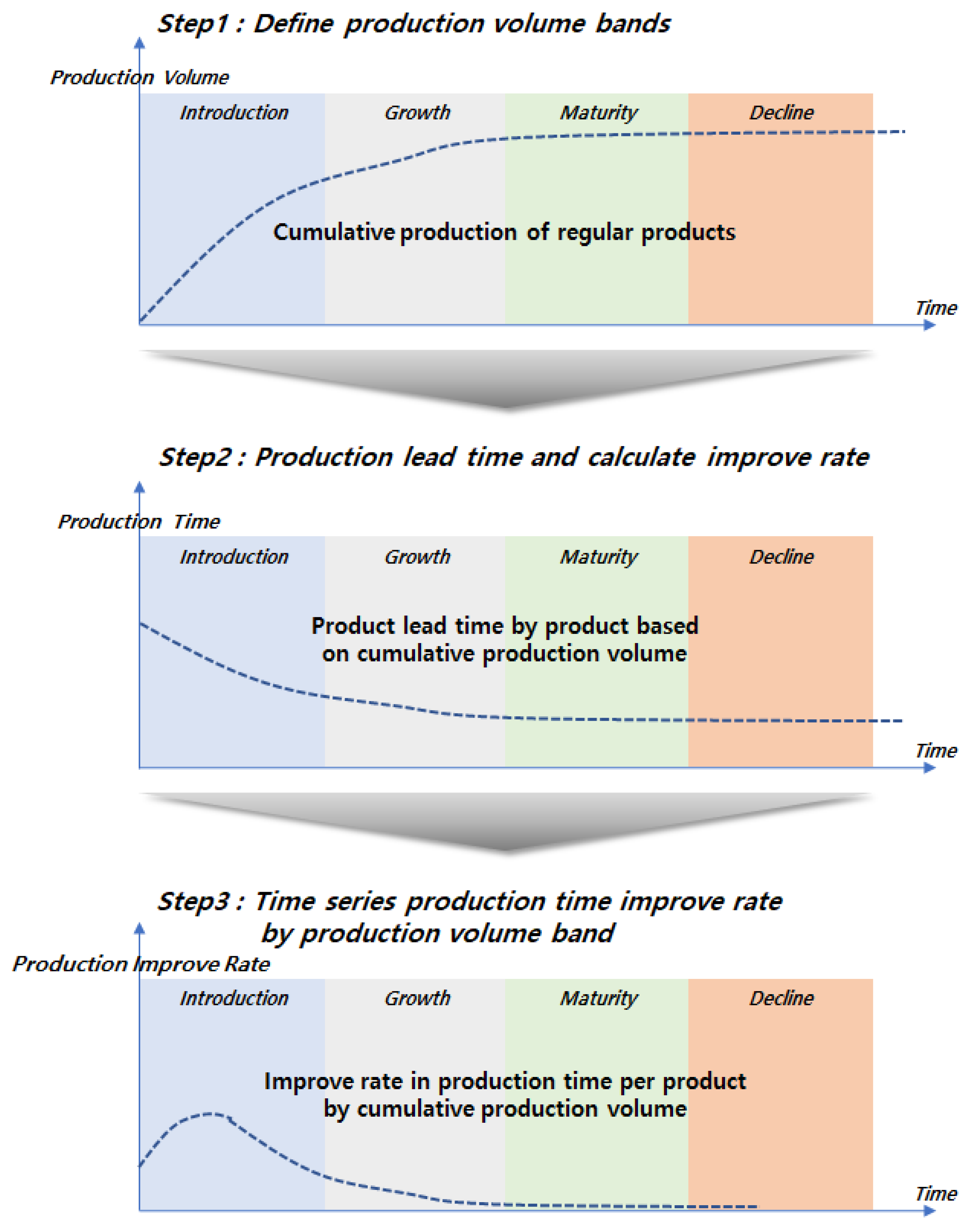
3. Production Improvement Rate with Time Series Data
3.1. Overall Structure
3.2. Production Improvement Procedures
4. Implementation and Results
4.1. Experiment Environments
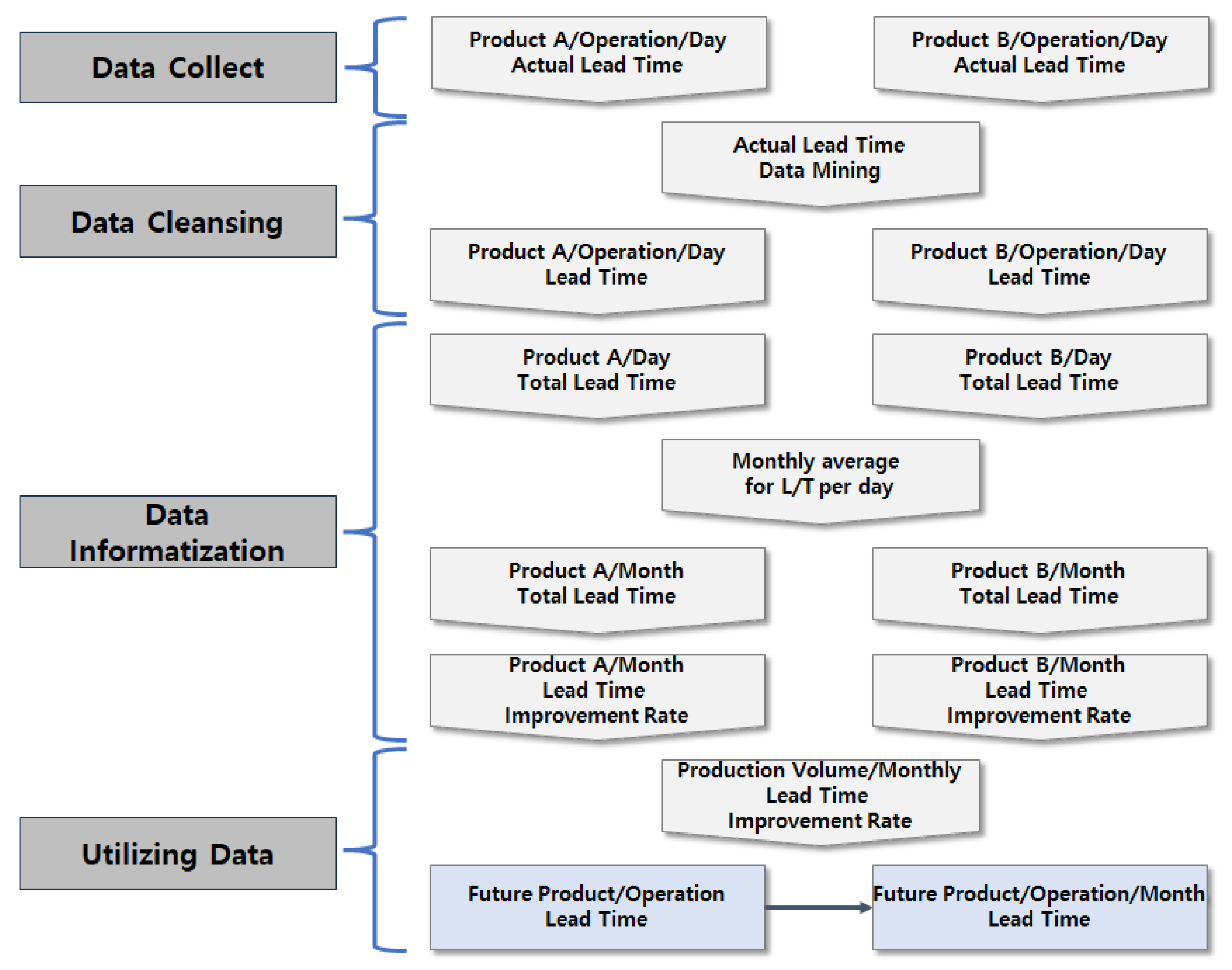
4.2. Data Processing
4.3. Aggregation of Production Time
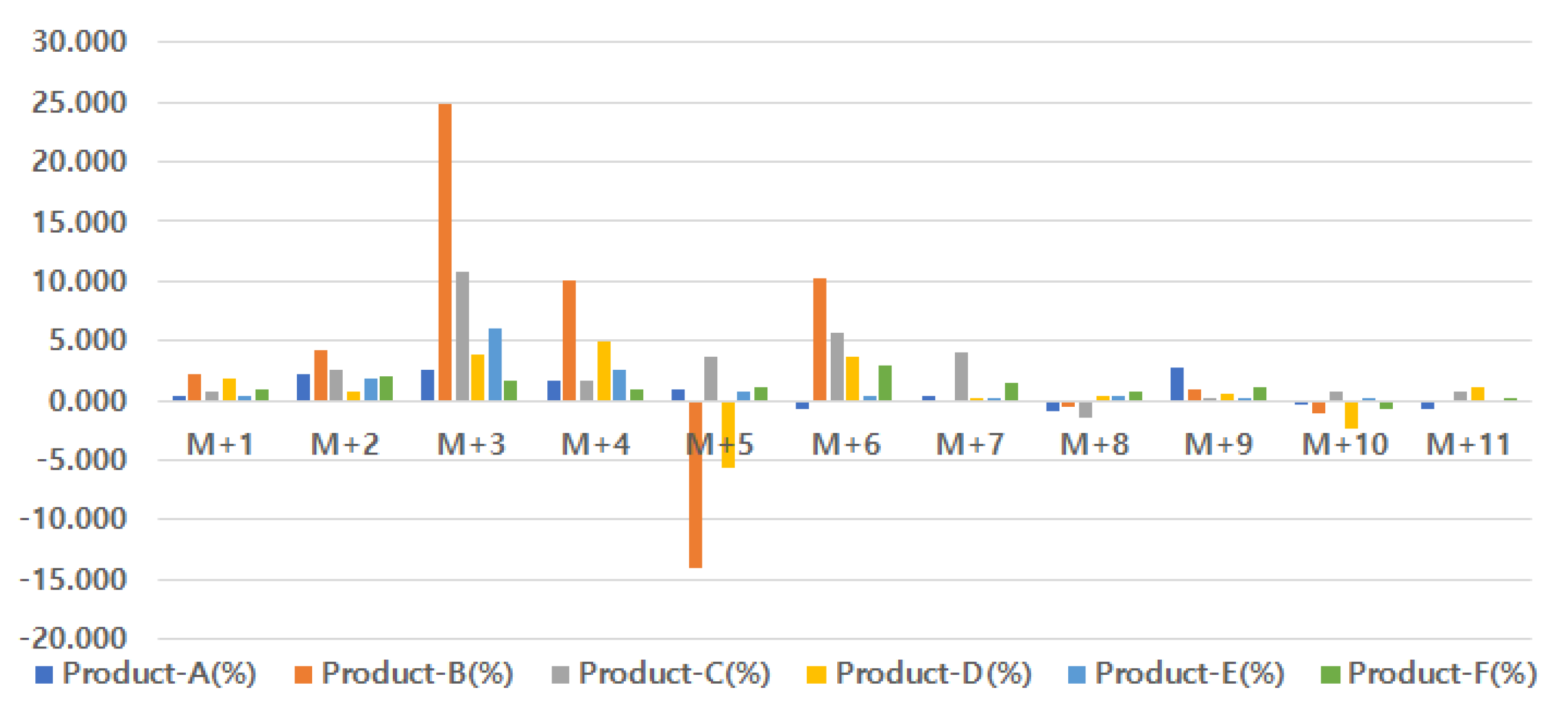
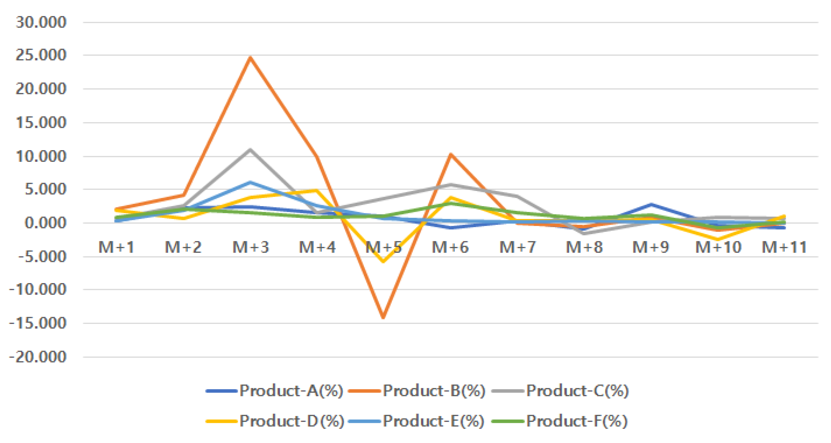
4.4. Calculation of Production Time Improvement Rate
4.5. Leverage Production Time Improvement Rate
4.6. Evaluation of The Experimental Method
5. Conclusions
Author Contributions
Funding
Institutional Review Board Statement
Informed Consent Statement
Data Availability Statement
Acknowledgments
Conflicts of Interest
References
- Bellgran, M.; Säfsten, K. Production Development-Design and Operation of Production Systems; Springer: Berlin/Heidelberg, Germany, 2010. [Google Scholar]
- Palange, A.; Dhatrak, P. Lean manufacturing a vital tool to enhance productivity in manufacturing. Mater. Today Proc. 2021, 46, 729–736. [Google Scholar] [CrossRef]
- Andersson, C.; Bellgran, M. On the complexity of using performance measures: Enhancing sustained production improvement capability by combining OEE and productivity. J. Manuf. Syst. 2015, 35, 144–154. [Google Scholar] [CrossRef]
- Rohani, J.M.; Zahraee, S.M. Production line analysis via value stream mapping: A lean manufacturing process of color industry. Procedia Manuf. 2015, 2, 6–10. [Google Scholar] [CrossRef]
- Sharma, K.M.; Lata, S. Effectuation of lean tool “5s” on materials and work space efficiency in a copper wire drawing micro-scale industry in India. Mater. Today Proc. 2018, 5, 4678–4683. [Google Scholar] [CrossRef]
- Veres, C.; Marian, L.; Moica, S.; Al-Akel, K. Case study concerning 5S method impact in an automotive company. Procedia Manuf. 2018, 22, 900–905. [Google Scholar] [CrossRef]
- Nallusamy, S. Execution of lean and industrial techniques for productivity enhancement in a manufacturing industry. Mater. Today Proc. 2021, 37, 568–575. [Google Scholar] [CrossRef]
- Arunagiri, P.; Suresh, P.; Jayakumar, V. Assessment of hypothetical correlation between the various critical factors for lean systems in automobile industries. Mater. Today Proc. 2020, 33, 35–38. [Google Scholar] [CrossRef]
- Bueno, A.; Godinho Filho, M.; Frank, A.G. Smart production planning and control in the Industry 4.0 context: A systematic literature review. Comput. Ind. Eng. 2020, 149, 106774. [Google Scholar] [CrossRef]
- Bonney, M. Reflections on production planning and control (PPC). Gest. Prod. 2000, 7, 181–207. [Google Scholar] [CrossRef]
- Wiendahl, H.H.; Von Cieminski, G.; Wiendahl, H.P. Stumbling blocks of PPC: Towards the holistic configuration of PPC systems. Prod. Plan. Control 2005, 16, 634–651. [Google Scholar] [CrossRef]
- Yin, Y.; Stecke, K.E.; Li, D. The evolution of production systems from Industry 2.0 through Industry 4.0. Int. J. Prod. Res. 2018, 56, 848–861. [Google Scholar] [CrossRef]
- Olhager, J.; Rudberg, M. Linking manufacturing strategy decisions on process choice with manufacturing planning and control systems. Int. J. Prod. Res. 2002, 40, 2335–2351. [Google Scholar] [CrossRef]
- Olhager, J. Evolution of operations planning and control: From production to supply chains. Int. J. Prod. Res. 2013, 51, 6836–6843. [Google Scholar] [CrossRef]
- Jacobs, R.F.; Berry, W.L.; Whybark, D.C.; Vollmann, T.E. Manufacturing planning and control for supply chain management: The CPIM Reference; McGraw-Hill Education: New York, NY, USA, 2018. [Google Scholar]
- Rondeau, P.; Litteral, L.A. The evolution of manufacturing planning and control systems: From reorder point to enterprise resource planning. Prod. Inventory Manag. J. 2001, 42. Available online: https://digitalcommons.butler.edu/cob_papers/41 (accessed on 27 September 2023).
- Nahmias, S.; Olsen, T.L. Production and Operations Analysis; Waveland Press: Long Grove, IL, USA, 2015. [Google Scholar]
- Lee, H.Y. Development of a Simulation-Based Smart-FAB Production Operating System Framework for the FAB Industries; Korea Advanced Institute of Science & Technology (KAIST): Daejeon, Republic of Korea, 2011. [Google Scholar]
- Ivert, L.K.; Jonsson, P. The potential benefits of advanced planning and scheduling systems in sales and operations planning. Ind. Manag. Data Syst. 2010, 110, 659–681. [Google Scholar] [CrossRef]
- Hvolby, H.H.; Steger-Jensen, K. Technical and industrial issues of Advanced Planning and Scheduling (APS) systems. Comput. Ind. 2010, 61, 845–851. [Google Scholar] [CrossRef]
- Venkatesh, J. An Introduction to Total Productive Maintenance (TPM); The Plant Maintenance Resource Center: Como, Italy, 2007; pp. 3–20. [Google Scholar]
- Chan, F.; Lau, H.; Ip, R.; Chan, H.; Kong, S. Implementation of total productive maintenance: A case study. Int. J. Prod. Econ. 2005, 95, 71–94. [Google Scholar] [CrossRef]
- Swanson, L. Linking maintenance strategies to performance. Int. J. Prod. Econ. 2001, 70, 237–244. [Google Scholar] [CrossRef]
- Agustiady, T.K.; Cudney, E.A. Total productive maintenance. In Total Quality Management & Business Excellence; Routledge: London, UK, 2018; pp. 1–8. [Google Scholar]
- Adesta, E.Y.; Prabowo, H.A.; Agusman, D. Evaluating 8 pillars of Total Productive Maintenance (TPM) implementation and their contribution to manufacturing performance. IOP Conf. Ser. Mater. Sci. Eng. 2018, 290, 012024. [Google Scholar] [CrossRef]
- Attri, R.; Grover, S.; Dev, N.; Kumar, D. Analysis of barriers of total productive maintenance (TPM). Int. J. Syst. Assur. Eng. Manag. 2013, 4, 365–377. [Google Scholar] [CrossRef]
- Banga, H.K.; Kumar, R.; Kumar, P.; Purohit, A.; Kumar, H.; Singh, K. Productivity improvement in manufacturing industry by lean tool. Mater. Today Proc. 2020, 28, 1788–1794. [Google Scholar] [CrossRef]
- Pagliosa, M.; Tortorella, G.; Ferreira, J.C.E. Industry 4.0 and Lean Manufacturing: A systematic literature review and future research directions. J. Manuf. Technol. Manag. 2021, 32, 543–569. [Google Scholar] [CrossRef]
- Dillon, A.P. A Study of the Toyota Production System: From an Industrial Engineering Viewpoint; Routledge: Oxfordshire, UK, 2019. [Google Scholar]
- Anoop, G.; Muhammed, V.S. A Brief Overview on Toyota Production System (TPS). Int. J. Res. Appl. Sci. Eng. Technol. 2020, 8, 2505–2509. [Google Scholar]
- Mabkhot, M.M.; Al-Ahmari, A.M.; Salah, B.; Alkhalefah, H. Requirements of the smart factory system: A survey and perspective. Machines 2018, 6, 23. [Google Scholar] [CrossRef]
- Meerkov, S.M.; Yan, C.B. Production lead time in serial lines: Evaluation, analysis, and control. IEEE Trans. Autom. Sci. Eng. 2014, 13, 663–675. [Google Scholar] [CrossRef]
- Rahman, S.u. Theory of constraints: A review of the philosophy and its applications. Int. J. Oper. Prod. Manag. 1998, 18, 336–355. [Google Scholar] [CrossRef]
- Scholl, A.; Voß, S. Simple assembly line balancing—Heuristic approaches. J. Heuristics 1997, 2, 217–244. [Google Scholar] [CrossRef]
- Prasad, S.; Khanduja, D.; Sharma, S.K. A study on implementation of lean manufacturing in Indian foundry industry by analysing lean waste issues. Proc. Inst. Mech. Eng. Part B J. Eng. Manuf. 2018, 232, 371–378. [Google Scholar] [CrossRef]
- Tersine, R.J.; Hummingbird, E.A. Lead-time reduction: The search for competitive advantage. Int. J. Oper. Prod. Manag. 1995, 15, 8–18. [Google Scholar] [CrossRef]
- Ghazavi, M.; Eghbali, A.H. New geometric average method for calculation of ultimate bearing capacity of shallow foundations on stratified sands. Int. J. Geomech. 2013, 13, 101–108. [Google Scholar] [CrossRef]


| TPM | |
|---|---|
| Object | Equipment (input and cause) |
| Means of attaining goal | Employee participation and equipment oriented |
| Target | Elimination of losses and waste |
| Distinguish | Monthly Production (Units) | Yearly Production (Units) | Note |
|---|---|---|---|
| Low | 0 to 500 | Under 5000 | Of the two divisions of production, yearly production is preferred |
| Medium | Over 500 to Under 10,000 | Over 5000 to Under 100,000 | |
| High | Over 10,000 | Over 100,000 |
| Hardware | Performance |
|---|---|
| CPU | Intel Xeon Gold 5220 @ 2.20 GHz |
| RAM | 512 GB |
| STORAGE | 50 TB (SSD) |
| Hardware | Performance |
|---|---|
| CPU | Intel i7-6700 @ 3.40 GHz |
| RAM | 32 GB |
| STORAGE | 256 GB (SSD) |
| Type | |
|---|---|
| OS | Windows 11 Home 22H2 |
| DBMS | Oracle 19 Client |
| Development Languages | Oracle PL/SQL |
| Development Tools | SQL Developer |
| Production Time | ||||||
|---|---|---|---|---|---|---|
| Month | Product-A | Product-B | Product-C | Product-D | Product-E | Product-F |
| M+0 | 2.970 | 2.359 | 3.045 | 3.321 | 2.024 | 2.064 |
| M+1 | 2.960 | 2.309 | 3.023 | 3.259 | 2.016 | 2.046 |
| M+2 | 2.895 | 2.211 | 2.945 | 3.236 | 1.978 | 2.004 |
| M+3 | 2.823 | 1.663 | 2.624 | 3.114 | 1.858 | 1.972 |
| M+4 | 2.777 | 1.497 | 2.581 | 2.962 | 1.812 | 1.954 |
| M+5 | 2.750 | 1.708 | 2.486 | 3.130 | 1.799 | 1.933 |
| M+6 | 2.770 | 1.532 | 2.344 | 3.013 | 1.793 | 1.876 |
| M+7 | 2.760 | 1.532 | 2.250 | 3.004 | 1.791 | 1.848 |
| M+8 | 2.785 | 1.541 | 2.285 | 2.994 | 1.785 | 1.834 |
| M+9 | 2.710 | 1.526 | 2.279 | 2.976 | 1.7838 | 1.813 |
| M+10 | 2.720 | 1.542 | 2.261 | 3.049 | 1.782 | 1.827 |
| M+11 | 2.740 | 1.543 | 2.246 | 3.0152 | 1.782 | 1.823 |
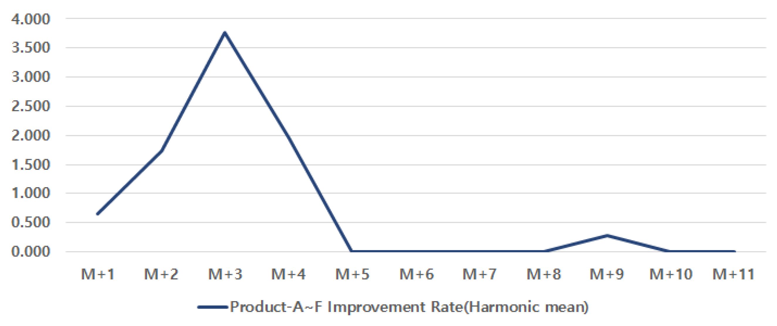
| Improvement Rate (%) for Products with Similar Production Volumes (High Volume) | |||||||
|---|---|---|---|---|---|---|---|
| Month | Product-A | Product-B | Product-C | Product-D | Product-E | Product-F | Products A∼F (Harmonic Mean) |
| M+1 | 0.337 | 2.120 | 0.732 | 1.855 | 0.366 | 0.858 | 0.648 |
| M+2 | 2.196 | 4.224 | 2.581 | 0.724 | 1.880 | 2.076 | 1.727 |
| M+3 | 2.504 | 24.785 | 10.884 | 3.764 | 6.061 | 1.590 | 3.771 |
| M+4 | 1.594 | 9.982 | 1.631 | 4.862 | 2.518 | 0.898 | 1.963 |
| M+5 | 0.990 | −14.061 | 3.692 | −5.671 | 0.718 | 1.087 | 0.000 |
| M+6 | −0.727 | 10.307 | 5.708 | 3.757 | 0.339 | 2.930 | 0.000 |
| M+7 | 0.361 | 0.000 | 4.010 | 0.289 | 0.100 | 1.509 | 0.000 |
| M+8 | −0.906 | −0.588 | −1.533 | 0.350 | 0.307 | 0.766 | 0.000 |
| M+9 | 2.693 | 0.935 | 0.228 | 0.575 | 0.080 | 1.158 | 0.287 |
| M+10 | −0.369 | −1.042 | 0.798 | −2.432 | 0.122 | −0.781 | 0.000 |
| M+11 | −0.735 | −0.032 | 0.681 | 1.102 | 0.000 | 0.194 | 0.000 |
| Time Series Production Time Information | ||
|---|---|---|
| Month | Improvement Rate | Production Time |
| M+0 | 0.000% | 4.000 |
| M+1 | 0.648% | 3.974 |
| M+2 | 1.727% | 3.905 |
| M+3 | 3.771% | 3.758 |
| M+4 | 1.963% | 3.684 |
| M+5 | 0.000% | 3.684 |
| M+6 | 0.000% | 3.684 |
| M+7 | 0.000% | 3.684 |
| M+8 | 0.000% | 3.684 |
| M+9 | 0.287% | 3.674 |
| M+10 | 0.000% | 3.674 |
| M+11 | 0.000% | 3.674 |
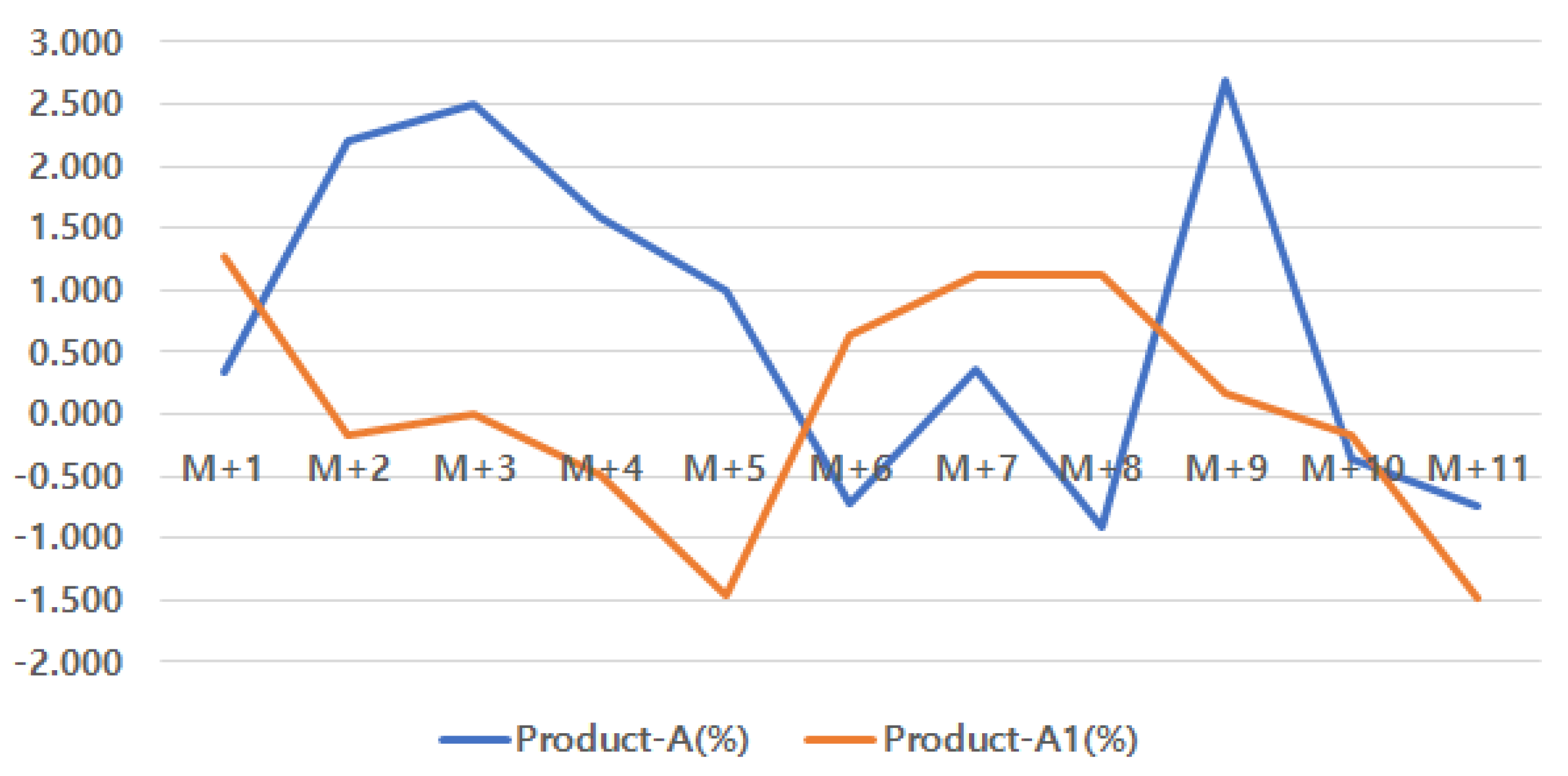
| Product-A | Product-A1 | |||
|---|---|---|---|---|
| Month | Production Time | Improvement Rate | Production Time | Improvement Rate |
| M+0 | 2.97 | 0.624 | ||
| M+1 | 2.96 | 0.377% | 0.616 | 1.282% |
| M+2 | 2.895 | 2.196% | 0.617 | −0.162% |
| M+3 | 2.8225 | 2.504% | 0.617 | 0.000% |
| M+4 | 2.7775 | 1.594% | 0.620 | −0.486% |
| M+5 | 2.75 | 0.990% | 0.629 | −1.452% |
| M+6 | 2.77 | −0.727% | 0.625 | 0.636% |
| M+7 | 2.76 | 0.361% | 0.618 | 1.120% |
| M+8 | 2.785 | −0.906% | 0.611 | 1.133% |
| M+9 | 2.71 | 2.693% | 0.610 | 0.164% |
| M+10 | 2.72 | −0.369% | 0.611 | −0.164% |
| M+11 | 2.74 | −0.735% | 0.620 | −1.473% |
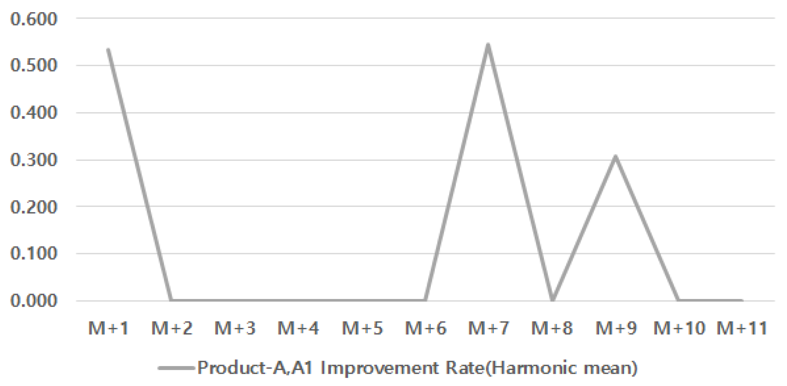
| Production Time Improvement Rate for Products with Different Production Volumes (Low and High Volume) | |||
|---|---|---|---|
| Month | Product-A Improvement Rate | Product-A1 Improvement Rate | Improvement Rate (Harmonic Mean) |
| M+1 | 0.377% | 1.282% | 0.533% |
| M+2 | 2.196% | −0.162% | 0.000% |
| M+3 | 2.504% | 0.000% | 0.000% |
| M+4 | 1.594% | −0.486% | 0.000% |
| M+5 | 0.990% | −1.452% | 0.000% |
| M+6 | −0.727% | 0.636% | 0.000% |
| M+7 | 0.361% | 1.120% | 0.546% |
| M+8 | −0.906% | 1.133% | 0.000% |
| M+9 | 2.693% | 0.164% | 0.309% |
| M+10 | −0.369% | −0.164% | 0.000% |
| M+11 | −0.735% | −1.473% | 0.000% |
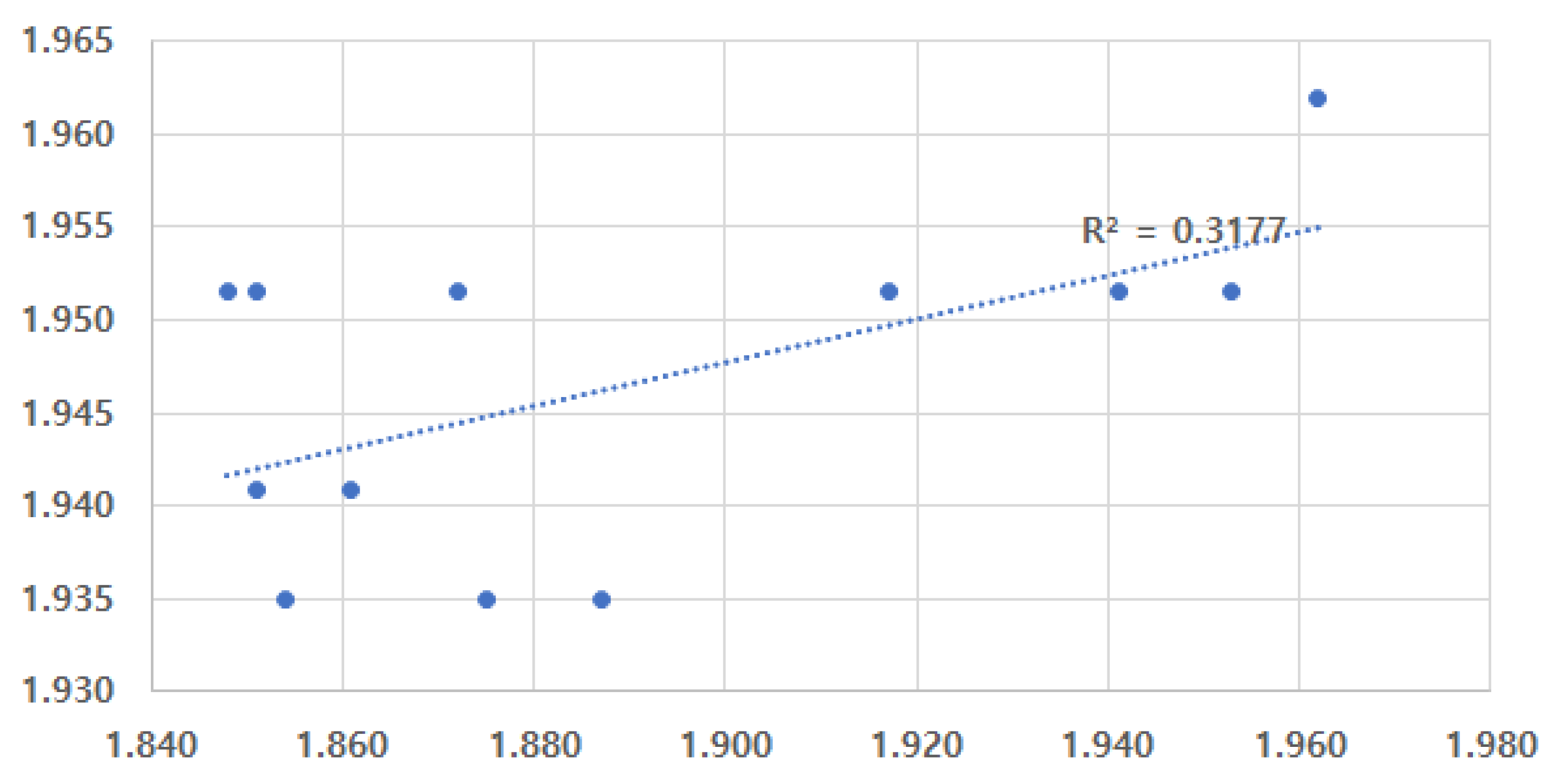
| Month | Product-G Actual Production Time | Products A∼F Improvement Rate | Product-G Predictions 1 | Products A, A1 Improvement Rate | Product-G Predictions 2 |
|---|---|---|---|---|---|
| M+0 | 1.962 | 0.000% | 1.962 | 0.000% | 1.962 |
| M+1 | 1.953 | 0.648% | 1.949 | 0.533% | 1.952 |
| M+2 | 1.941 | 1.727% | 1.916 | 0.000% | 1.952 |
| M+3 | 1.917 | 3.771% | 1.843 | 0.000% | 1.952 |
| M+4 | 1.872 | 1.963% | 1.807 | 0.000% | 1.952 |
| M+5 | 1.848 | 0.000% | 1.807 | 0.000% | 1.952 |
| M+6 | 1.851 | 0.000% | 1.807 | 0.000% | 1.952 |
| M+7 | 1.851 | 0.000% | 1.807 | 0.546% | 1.941 |
| M+8 | 1.861 | 0.000% | 1.807 | 0.000% | 1.941 |
| M+9 | 1.887 | 0.287% | 1.802 | 0.309% | 1.935 |
| M+10 | 1.875 | 0.000% | 1.802 | 0.000% | 1.935 |
| M+11 | 1.854 | 0.000% | 1.802 | 0.000% | 1.935 |
| Prediction 1 correlation coefficient | 0.936 | Prediction 2 correlation coefficient | 0.564 |
Disclaimer/Publisher’s Note: The statements, opinions and data contained in all publications are solely those of the individual author(s) and contributor(s) and not of MDPI and/or the editor(s). MDPI and/or the editor(s) disclaim responsibility for any injury to people or property resulting from any ideas, methods, instructions or products referred to in the content. |
© 2023 by the authors. Licensee MDPI, Basel, Switzerland. This article is an open access article distributed under the terms and conditions of the Creative Commons Attribution (CC BY) license (https://creativecommons.org/licenses/by/4.0/).
Share and Cite
Ki, I.; Song, H.; Ryu, J.; Jeong, J. Production Improvement Rate with Time Series Data on Standard Time at Manufacturing Sites. Appl. Sci. 2023, 13, 10937. https://doi.org/10.3390/app131910937
Ki I, Song H, Ryu J, Jeong J. Production Improvement Rate with Time Series Data on Standard Time at Manufacturing Sites. Applied Sciences. 2023; 13(19):10937. https://doi.org/10.3390/app131910937
Chicago/Turabian StyleKi, Injong, Hasup Song, Jihyeok Ryu, and Jongpil Jeong. 2023. "Production Improvement Rate with Time Series Data on Standard Time at Manufacturing Sites" Applied Sciences 13, no. 19: 10937. https://doi.org/10.3390/app131910937
APA StyleKi, I., Song, H., Ryu, J., & Jeong, J. (2023). Production Improvement Rate with Time Series Data on Standard Time at Manufacturing Sites. Applied Sciences, 13(19), 10937. https://doi.org/10.3390/app131910937