A DDPG-Based USV Path-Planning Algorithm

Abstract

Path planning is crucial in the automatic navigation of USVs (unmanned underwater vehicles), which directly affects the operational efficiency and safety of USVs. In this paper, we propose a path-planning algorithm based on DDPG (Deep Deterministic Policy Gradient) and make a detailed comparison with the traditional A-Star algorithm and the recent Actor–Critical algorithm. Through a series of simulation experiments, it can be observed that the optimal path for USVs found by the DDPG-based path planning algorithm is faster and more accurate than that found by the other two methods. The experimental results show that the DDPG algorithm has a significant advantage in processing time and better performance in terms of path quality and safety. These results provide a strong reference for future research on automatic navigation for USVs and demonstrate the potential of DDPG-based path planning for USVs.

1. Introduction

USVs represent a specialized category of compact, multifunctional, and intelligent unmanned marine platforms, which can be remotely piloted or operated autonomously to execute extensive and enduring marine operations in complex and dangerous waters. For proficient path planning in USVs, a system is required to ensure navigation between two designated points (such as start and target locations) and includes obstacle-avoidance capabilities (Cho et al., 2019; Liu et al., 2019; Woo et al., 2020) [1,2,3]. The efficiency of path planning has a profound impact on the overall quality of the routes created by the USV within its surroundings.

Path-planning strategies can be segmented into two primary types, specifically global and local methods, contingent on environmental visibility (Hong et al., 2011; Yao et al., 2017) [4,5]. Global methods are designed for conditions with only static hindrances and complete availability of environmental information in advance. They permit the pre-calculation of the briefest trajectory from the starting to the ending point using classical methods such as the A-star and Dijkstra algorithms (Song et al., 2019; Singh et al., 2018) [6,7]. They offer strong convergence and consistency, but they are primarily suitable for static surroundings and, therefore, require further refinement for generating USV-compatible paths (Bibuli et al., 2018) [8].

For instance, by refining the paths planned by the A-star algorithm through spline fitting, the feasibility of unmanned diving vessels can then be enhanced (Gul et al., 2018) [9]. However, these methods formulate trajectories by linking unidirectional points linearly, which are commonly at a low resolution, making them inapplicable in dynamic settings with moving obstructions. They also usually exhibit a high time complexity, making them challenging in vast environments.

In contrast, local methods fit dynamic situations better (Yu et al., 2021) [10]. These methods do not rely on prior information about the environment and are capable of finding high-resolution paths even when mobile objects are present.

Traditional approaches to USV path planning comprise heuristic search-based methods, minimum spanning tree-based methods, and neural network-based methods. Heuristic search-based strategies utilize algorithms like A* and Dijkstra for optimal USV path discovery, but they may suffer from premature convergence and local optimality. Therefore, it is suggested that algorithms, as well as the introduction of intelligent algorithms such as genetic and particle swarm algorithms, should be enhanced (Wang et al., 2021; Fang et al., 2021) [11,12].

Minimum spanning tree-based approaches, including Prim’s and Kruskal algorithms (Prim, 1957; Kruskal, 1956) [13,14], utilize graph theory to calculate the USV’s optimal path. In contrast, neural network-based methods utilize artificial neural networks for path modeling and calculation (Song et al., 2019; Duguleana et al., 2016) [15,16]. The development of technology has brought increasing attention to neural networks.

ML focuses on developing algorithms to enable computers to learn and make their own decisions based on data (Abdalzaher et al., 2023) [17]. RL (Reinforcement Learning), a branch of machine learning, focuses on actions derived from environmental interactions that amplify anticipated gains (Kaelbling et al., 1996) [18]. It is influenced by psychological behaviorists, whose theories concern how organisms, motivated by rewards or penalties from their surroundings, develop their expectations and form habits to maximize benefits. RL is a learning approach wherein an agent learns, which correlates states to actions to optimize rewards. The agent should continually test and adapt within the environment, employing feedback (rewards) to refine the state-action alignment. Thus, trial and error, along with delayed rewards, represent RL’s key features. In machine learning, the primary methods are supervised and unsupervised learning (Li, 2017) [19]. An RL system typically comprises four elements: Policy, Reward, Value, and Environment or Model. The policy outlines intelligent behaviors for a particular state, essentially mapping the state to the corresponding action. The state encompasses both the environmental and intelligent states, which start from the intelligence perceived. The reward signal signifies the RL problem’s goal, where the scalar value from the environment is the main influence on the strategy. The value function assesses long-term gains, while the external environment is often referred to as the model (Model) (Sarker, 2021) [20].

Wang et al. (2018) [21] employed a strategy that assigned probabilities to eight discrete actions based on their reward values, devising a Q-learning-based path planning algorithm. However, this method suffers from slow convergence and extensive iterations. Wu et al. (2020) [22] utilized state value functions and action dominance functions to assess Q, constructing a dual Q-based ANOA algorithm to minimize DQN’s coupling (Sarker, 2021) [23]. Hado Hasselt (2010) [24] designed a novel off-policy RL algorithm, Double Q-learning, to mitigate overestimations introduced by positive bias in specific stochastic settings. Despite notable enhancements in precision and efficiency compared with traditional techniques, these approaches have partially addressed USV path planning but remain constrained as USV technology advances.

Silver et al. (2014) [25] presented deterministic policy gradient algorithms for RL in continuous action contexts. Lillicrap et al. (2015) established DDPG [26], merging the actor-critic method with insights from the DQN (Deep Q Network)’s recent success (Zhu et al., 2021) [27]. We introduce an advanced path-planning methodology anchored in DDPG. Using the target position to guide USV in environment exploration, we enhance the learning pace. Substituting collision penalties with reward incentives fosters rapid learning in obstacle avoidance for the unmanned vessel.

USV route planning often involves continuous decision making, including the option from an infinite range of actions rather than a finite set. DDPG is designed for continuous action spaces and is suitable for USV route planning, which often requires continuous decisions such as speed and steering angle selection. In addition, DDPG utilizes a deterministic strategy that directly generates optimal action values instead of action distributions, eliminating the need for distribution sampling and thus speeding up learning. Combined with experience replay, DDPG allows the algorithm to learn from previous experience, which improves the stability of learning. By using the current network and the target network, DDPG reduces policy fluctuations and improves learning stability, which is particularly beneficial in scenarios with a continuous action space. In certain cases that involve continuous action spaces, for instance, DDPG may outperform traditional behavioral methods in terms of convergence speed and final performance. We therefore used DDPG as an extended model for our experiments.

This article is divided into four chapters. Section 1, Methodology, introduces the DDPG algorithm and the USV motion model in detail; Section 2, Simulation, provides a detailed introduction to the USV State Space and environment modeling of the USV; Section 3, Discussion, shows the results of simulation testing; Section 4, Conclusion, indicates the research conclusions and future improvement directions of the algorithm.

2. Methodology

2.1. DDPG

DDPG (The Deep Deterministic Policy Gradient algorithm) is an enhancement of the DPG (Deterministic Policy Gradient algorithm), inheriting its deterministic policy gradient. In this framework, an intelligent body determines specific actions based on state decisions, utilizing a deep neural network to bolster the decision function fitting. Unlike stochastic policies, DDPG significantly diminishes the required amount of sampled data, thereby improving algorithm efficiency and promoting intelligent learning within continuous action spaces.

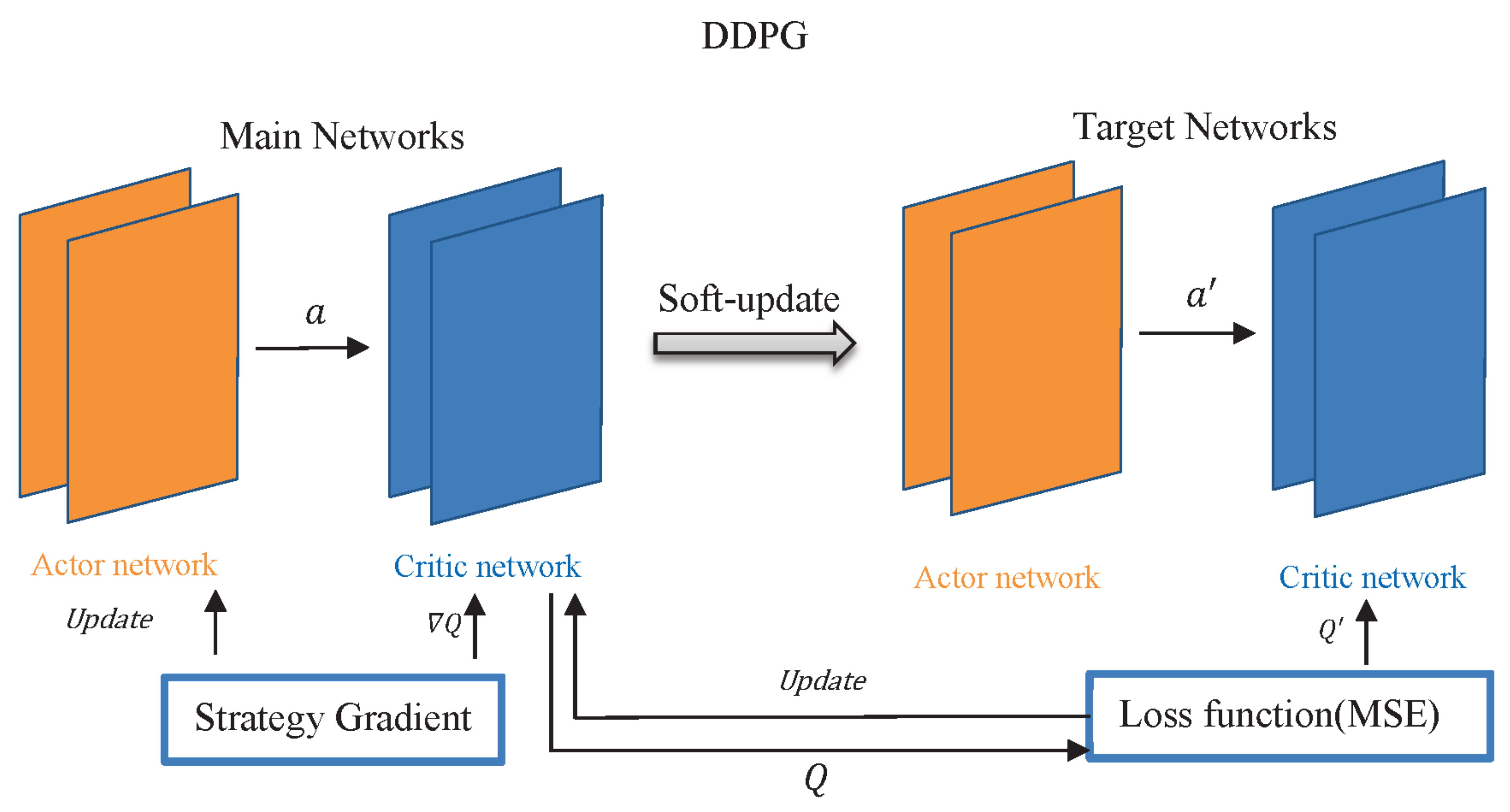
Adhering to an Actor–Critic architecture, the DDPG algorithm primarily consists of two components: the Actor network and the Critic network. The Actor network focuses on generating actions and mediating environmental interactions for the USV, while the Critic network evaluates state and action performance. The insights from this evaluation guide the policy function to formulate the subsequent phase of actions. Both the Actor and Critic components operate through a dual network structure, employing target and eval networks. The overall structure of the DDPG algorithm is visually depicted in Figure 1. The symbols and their meanings of DDPG are detailed in

Table 1. DDPG Symbol Definition Table.

Symbol	Description
${\theta }^u$	Parameter vector for the policy network in the Actor-eval network, subject to recurrent modification.
a	Action chosen by the Actor-eval network based on the current state s.
$s$	The prevailing state in the environment.
$s^{\prime }$	The ensuing state resulting from the execution of action a in the environment.
$r$	The reward received as a consequence of the current action’s execution.
${\theta }^{u^{\prime }}$	Parameter vector for the policy network in the Actor-target network, periodically copied from ${\theta }^u$.
$a^{\prime }$	Best subsequent action chosen by the Actor-target network based on the following state $s^{\prime }$.
${\theta }^Q$	Parameter vector for the Critic-eval network, subject to repeated refinement.
$y_i$	The target Q value calculated in the Critic-eval network using Equation (1).
$\gamma$	Discount factor that determines the importance of future rewards in the learning process.
$Q^{\prime }\left(s^{\prime },a^{\prime },{\theta }^{Q^{\prime }}\right)$	Q value estimated by the Critic-target network, with  ${\theta }^{Q^{\prime }}$ representing its principal parameter.
$s_t$	The state of the Unmanned Surface Vehicle (USV) at time t.
$\mu \left(\left.s_t\right|{\theta }^{\mu }\right)$	The real-time action emitted by the Actor-eval network based on state  $s_t$ and parameter ${\theta }^{\mu }$.
$a_t$	The action taken at time t.
${\mu }^{\prime }\left(\left.s_{t+1}\right|{\theta }^{\mu }{}^{\prime }\right)$	The Q value produced by the Critic-eval network for state  $s_t$ and action $a_t$ with parameter ${\theta }^Q$.
$Q^{\prime }\left(s_{t+1},{\mu }^{\prime }\left.\left(\left.s_{t+1}\right|{\theta }^{\mu }{}^{\prime }\right)\right|{\theta }^{Q^{\prime }}\right)$	The objective Q value generated by the Critic-target network for state $s_{t+1}$ and the action ${\mu }^{\prime }$.
${\rho }^{\beta }\left(S\right)$	The distribution of states S created by the agent-centric behavioral strategy $\beta$.
${\theta }^u\left(S,\mu \left(S\right)\right)$	Parameters representing the policy network’s strategy function μ for state S.
$J_{{\beta }_{\left(\mu \right)}}$	The performance metric or performance objective, which measures the efficacy of policy μ.
$\beta$	The behavior policy, which introduces stochastic noise into action decision-making during reinforcement learning training.
${\theta }^{Q^T}$	Target network parameters for the Critic.
$\tau$	A parameter used in the soft update algorithm.
${\theta }^{Q^0}$	Initial target network parameters for the Critic.
${\theta }^k$	Parameters for the eval network in the Critic.
$L$	The loss of the Critic network, computed as the mean square error.
$N$	The number of data samples in the batch.
$R_i$	Reward for a specific transition.
${\mu }^{\prime }$	Target network parameters in the Critic.
$Q^{\prime }$	Parameters of the target network in the Actor.
${\nabla }_{{\theta }^{\mu }}{J}_{\beta \left(\mu \right)}$	The gradient of the performance objective with respect to the parameters of the Actor’s policy network.
${\nabla }_{a}Q{\left.\left(s,\left.a\right|{\theta }^Q\right)\right|}_{a=\mu \left(s_{\mathrm{i}}\right)}$	The gradient of the Q function with respect to the action.
$\nabla {\theta }^{\mu }\mu \left(\left.s\right|{\theta }^{\alpha }\right)$	The gradient of the policy network in the Actor.
$E_{s-\rho }\beta$	Expected value under the distribution of states according to the behavioral strategy $\beta$.
${\rho }^{\beta }$	The distribution function associated with the agent’s behavioral policy.

, the DDPG Symbol Definition Table.

In Figure 1, the network known as Actor-eval primarily deals with the recurrent modification of the policy network parameter denoted by ${\theta }^u$. It chooses action a based on the prevailing state $s$, generating the ensuing state $s^{\prime }$ and reward $r$ as a consequence of the current action’s execution during environmental interaction. Concurrently, the Actor-target network has the duty of identifying the best subsequent action $a^{\prime }$, relying on the following state $s^{\prime }$, which is sampled from the stored experiences. Periodic copying from ${\theta }^u$ in the Actor-eval network to ${\theta }^{u^{\prime }}$ in the Actor-target network is undertaken. Additionally, the Critic-eval network is fundamentally engaged in the repeated refinement of the network parameters ${\theta }^Q$ through calculation of the present $Q$ value:

$$y_i=r_i+\gamma Q^{\prime }\left(s^{\prime },a^{\prime },{\theta }^{Q^{\prime }}\right)$$

(1)

where the variable $\gamma$ signifies a discount factor impacting the priority given to future over present rewards in the learning process. In the Critic-target network, the principal parameter ${\theta }^{Q^{\prime }}$ is derived by periodically duplicating the ${\theta }^Q$ parameter, taking primary responsibility for evaluating $Q^{\prime }\left(s^{\prime },a^{\prime },{\theta }^{Q^{\prime }}\right)$.

Given that the state of the USV is $s_t$ and the action occurs at time $t$, the following operations are conducted:

• The Actor-eval network emits real-time actions $\mu \left(\left.s_t\right|{\theta }^{\mu }\right)$, which are enforced by the USV to engage with the environment;
• The Critic-eval network produces $Q$ values $Q\left(s_t,\left.a_t\right|{\theta }^Q\right)$, utilized to assess the present state-action’s worth;
• The Actor-target network delivers ${\mu }^{\prime }\left(\left.s_{t+1}\right|{\theta }^{\mu }{}^{\prime }\right)$, calculating the destination Q value from the next optimal action $a^{\prime }$ for state $s_{t+1}$ in the observation replay reservoir;
• The Critic-target network generates the objective Q value $Q^{\prime }\left(s_{t+1},{\mu }^{\prime }\left.\left(\left.s_{t+1}\right|{\theta }^{\mu }{}^{\prime }\right)\right|{\theta }^{Q^{\prime }}\right)$, and the UAV receives environmental rewards to derive the target $Q$ value.

The elementary notions linked to the DDPG algorithm encompass:

• Deterministic Action Strategy $\mu$: A function to calculate actions at each phase as $a_t=\mu \left(s_t\right)$.
• Policy Network: This neural network emulates the function $\mu$, termed a strategy network with parameters ${\theta }^{\mu }$.
• Performance Metric $J$: Also known as the performance objective, it gauges policy $\mu$’s efficacy. In an off-policy setting, it is described by

  $$J_{{\beta }_{\left(\mu \right)}}={{\displaystyle \int }}_S{\rho }^{\beta }\left(S\right){\theta }^u\left(S,\mu \left(S\right)\right)dx=E_{s-p}\beta \left[Q^{\mu }\left(s,\mu \left(s\right)\right)\right]$$

  (2)

  In this expression, $S$ is the state created by the Agent-centric behavioral strategy; ${\rho }^{\beta }$ is its distribution; $Q^{\mu }\left(s,\mu \left(s\right)\right)$ indicates the $Q$ value resulting from choices under strategy $\mu$.
• Strategy Gradient Definition: This represents the gradient of performance objective function $J$ relative to ${\theta }^{\mu }$.
• Action-value Function (Q Function): In state $s_t$, following action $a_t$, and persistently applying policy $\mu$, the anticipated value of $R_t$ is

  $$Q^{\mu }\left(s_t,a_t\right)=E\left[r\left(s_t,a_t\right)+\gamma Q^{\mu }\left(s_{t+1},\mu \left(s_{t+1}\right)\right)\right]$$

  (3)

During the training phase of RL, the exploration of potentially superior strategies necessitates the introduction of stochastic noise into the action’s decision-making protocol. This transformation alters the decision of action from a fixed pattern to a probabilistic one. Actions are then drawn from this probabilistic process and forwarded to the environment for implementation. This approach is referred to as the behavior policy, symbolized by $\beta$, and categorized as off-policy. The UO (Uhlenbeck–Ornstein) random procedure, notable for its excellent correlation in temporal sequences, enables effective environmental exploration by the agent. Hence, in the context of this study, the UO stochastic process is employed for DDPG training.

Concerning the training of the network, DDPG’s focus lies in the continuous training and enhancement of the eval parameters within both Actor and Critic. Subsequently, after a specific duration, the target network’s parameters are rejuvenated through the soft update algorithm. The updated formulation can be expressed as

$$soft-update\left\{\begin{array}{c}{\theta }^{Q^T}\Leftarrow \tau {\theta }^Q+\left(1-\tau \right){\theta }^{Q^0}\\ {\theta }^k\Leftarrow \tau {\theta }^{\mu }+\left(1-\tau \right){\theta }^u\end{array}\right.$$

(4)

Here, ${\theta }^{Q^{\prime }}$ and ${\theta }^{{\mu }^{\prime }}$ correspond to the target network parameters, while ${\theta }^Q$ and ${\theta }^{\mu }$ are linked to eval network parameters. The parameter $\tau$ is commonly set to 0.001. In the context of refining the parameters for the updated Critic network, the Critic network’s loss is conceived as the MSE (mean square error), represented as

$$L=\frac{1}{N}{\displaystyle \sum }_i{\left(y_i-Q\left(S_i,a\left.z\right|{\theta }^Q\right)\right)}^2$$

(5)

In this expression, $y_i$. is delineated as

$$y_i=R_i+\tau Q^{\prime }\left(S_{i+1},{\mu }^{\prime }\left.\left(\left.s_{i+1}\right|{\theta }^{{\mu }^{\prime }}\right)\right|{\theta }^{Q^{\prime }}\right)$$

(6)

Here, ${\mu }^{\prime }$ signifies the target network’s parameters in the Critic, and $Q^{\prime }$ represents the parameters of the target network in the Actor. The term $y_i$ is perceived as a ‘tag’, with network parameters adjusted via the back-propagation algorithm throughout the training phase. Regarding the policy gradient computation for the Actor, it can be illustrated as

$${\nabla }_{{\theta }^{\mu }}{J}_{\beta \left(\mu \right)}\approx E_{s-\rho }\beta \left[{\nabla }_{a}Q{\left.\left(s,\left.a\right|{\theta }^Q\right)\right|}_{a=\mu \left(s_{\mathrm{i}}\right)}·\nabla {\theta }^{\mu }\mu \left(\left.s\right|{\theta }^{\alpha }\right)\right]$$

(7)

The gradient of the strategy is represented by the expected value of ${\nabla }_{a}Q·\nabla {\theta }^{\mu }\mu$, under the condition where $S$ follows the distribution of ${\rho }^{\beta }$. Utilizing the Monte Carlo algorithm, it is possible to estimate ${\nabla }_{a}Q·\nabla {\theta }^{\mu }\mu$. The information concerning (transition) state transitions, contained within the empirical storage mechanism, denoted as $⟨s,a,r,s^{\prime }⟩$, is derived from the agent’s behavior policy $\beta$, with the corresponding distribution function ${\rho }^{\beta }$. Hence, when extracting mini-batch data randomly from the replay memory buffer, the Monte Carlo method enables this data to serve as an unbiased approximation of the above-mentioned expectation. This is achieved by applying the previous policy gradient equation. Therefore, the expression for the strategy gradient can be formulated as

$${\nabla }_{\theta \mu }{J}_{\beta \left(\mu \right)}\approx \frac{1}{N}\sum _i\hspace{0.17em}\left({\left.{\left.{\nabla }_{a}Q\left(s,a\mid {\theta }^Q\right)\right|}_{s=s_i,a=\mu \left(s_i\right)}\cdot {\nabla }_{\theta \mu }\mu \left(s,{\theta }^{\mu }\right)\right|}_{s=s_i}\right)$$

(8)

The following section will present the pseudocode representation corresponding to the DDPG algorithm (Algorithm 1).

Algorithm 1 DDPG based on USV

Require: The number of episodes for training $U$, frequency of training $\mathrm{K}$, the size of experience buffer $\mathrm{EN}$,    the number of sequences for the first sampling $\mathrm{S}$, and the regulator factor of the first sampling a. The    number of samples for the second sampling $\mathrm{M}$, the regulator factor of the second sampling $\mathrm{b}$. the    discount factor of reward $\mathrm{c}$, the end time of training $T$, the update frequency of target $Q$ network $\mathrm{L}$. Ensure: Optimal network parameters.   Initialize the parameters of Online Policy Net and Target Policy Net with ${\theta }^{\pi }$ and ${\theta }^{{\pi }^{\prime }}$, the parameters of Online $Q$ Net and Target $Q$ Net with ${\theta }^{°}$ and ${\theta }^{\mathrm{C}}$.   Initialize experience buffer $E$, the number of sequences in the experience buffer $Ei$, the storage experience buffer of a single sequenceh, the priority $p_1$.   for episode $=1,U$ do     Initialize a OU process, ${\tau }_t$ for action exploration.     Receive initial observation state $s_1$.     for $t=1, T$ do       Select action $a_t=\pi \left(s_t\mid {\theta }^{\pi }\right)+{\mu }_t$ according to the online policy and exploration noise.       Execute action at and observe new state $s_{t+1}$.       Store transition $\left(s_t,a_t,r_t,s_{t+1}\right)$ in experience buffer $E$.       if $t\% K=0$ and episode $>U$ then         for $i=1, N$ do            Calculate the probability of each sample $P\left(i\right)=\frac{\pi }{\sum in}$            Based on sampling probability P(i), S sequences are sampled from E and stored in experience buffer $E$.            for $i=1 S$ do               Calculate the probability of each sample  $P_s\left(u\right)=\frac{P_{su}^{\beta }}{{{\displaystyle \sum }}_{k-1}^N{P}_{sk}^{\beta }}$               Based on sampling probability $P_s\left(u\right)$, M sequences are sampled from $E$ and stored in experience buffer $S$               Using samples in S, Minimize the loss function to update the critic network:                         $L_i=\frac{1}{N}{\displaystyle \sum _i}\hspace{0.17em}{\left(y_i-Q\left(s_i,a_i\mid {\theta }^Q\right)\right)}^2$               Update the online policy using the sampled policy gradient:                 ${\nabla }_{\theta \mu }{J}_{\beta \left(\mu \right)}\approx \frac{1}{N}{\displaystyle \sum _i}\hspace{0.17em}\left({\left.{\left.{\nabla }_{a}Q\left(s,a\mid {\theta }^Q\right)\right|}_{s-s_i,a-\mu \left(s_i\right)}\cdot {\nabla }_{\theta \mu }\mu \left(s,{\theta }^{\mu }\right)\right|}_{s-s_i}\right)$               Update the target networks:                         $\begin{array}{c}\hfill {\theta }^{Q^{\prime }}\leftarrow \tau {\theta }^Q+\left(1-\tau \right){\theta }^{Q^{\prime }}\\ \hfill {\theta }^{{\pi }^{\prime }}\leftarrow \tau {\theta }^{\pi }+\left(1-\tau \right){\theta }^{{\pi }^{\prime }}\end{array}$

2.2. Motion Model for Unmanned Surface Vehicles

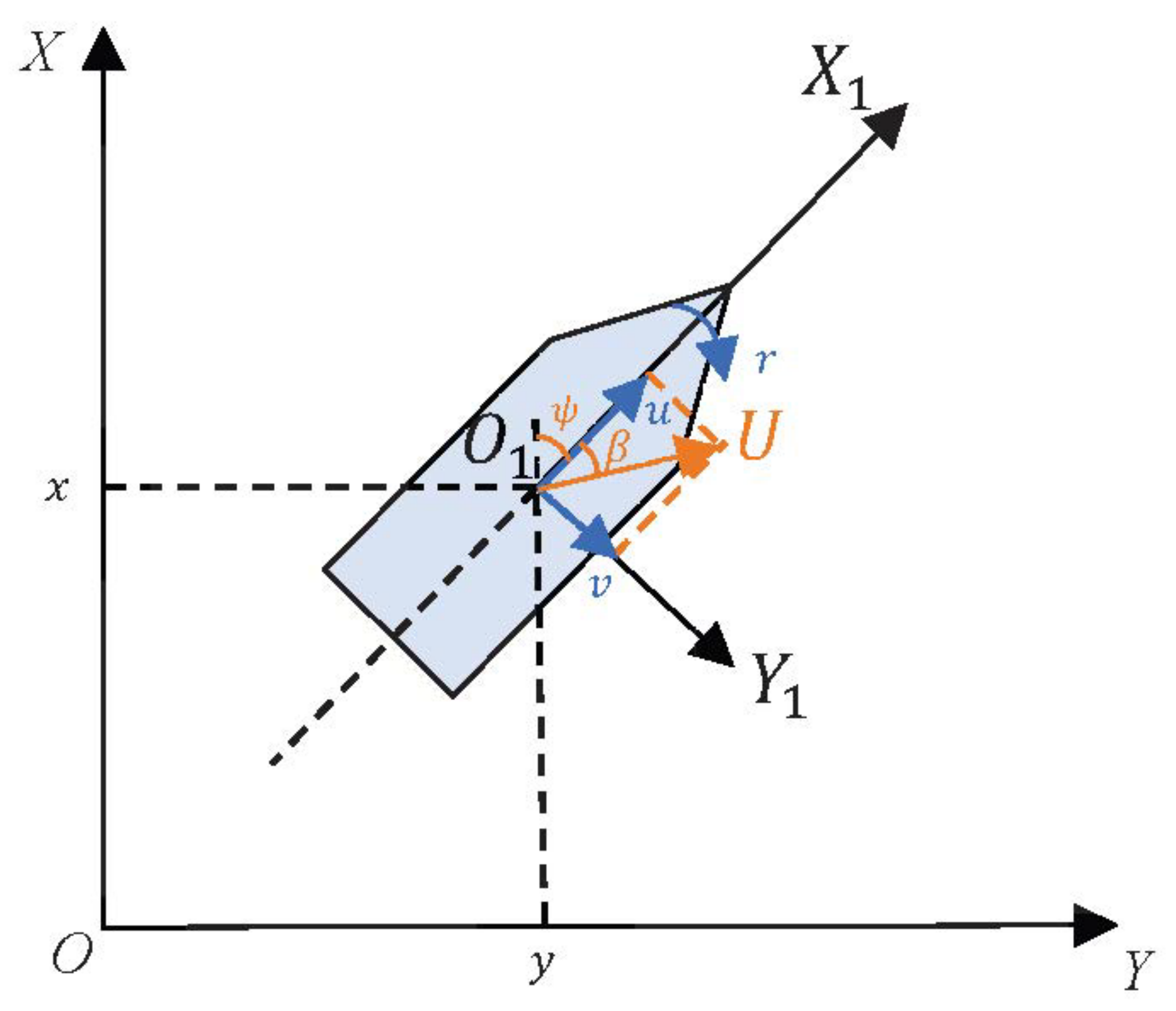
In this study, an underactuated USV is employed as the subject of research for path planning. The position of the USV within the Earth’s coordinate system is depicted by the position state vector $\eta ={\left[x y \psi \right]}^T$, where $\left(x,y\right)$ signifies the location, and $\psi$ denotes the orientation angle. The horizontal velocity of the USV is represented by the velocity vector $v={\left[u v r\right]}^T$, in which $u,v$, and $r$ correspond to the forward velocity, lateral velocity, and yaw rate, respectively.

To create a simplified model of the USV that is conducive to the design of a path planning system, the following assumptions have been adopted:

• The USV exhibits six degrees of freedom: heave, sway, yaw, roll, pitch, and surge. The last three have a minimal influence on the USV and are thus disregarded.
• The USV’s mass is uniformly distributed, and it is symmetric with respect to the OXZ plane; that is, $I_{xy}=I_{yz}=0$.
• The origin of the body coordinate system is located at the center of the USV.
• An underactuated ship refers to one that cannot generate thrust in the lateral direction (or has transverse thrusters that are inoperative for other reasons). It has a longitudinal propeller only. Therefore, the thrust vector $\tau$ can be expressed as ${\left[{\tau }_u 0 {\tau }_r\right]}^r$, where ${\tau }_u$ is the main propulsion thrust, and ${\tau }_r$ is the turning moment induced by the rudder. As no force is applied in the lateral direction, the value is zero.
• Higher-order hydrodynamic terms are disregarded.

Based on these simplifications, the nonlinear three-degree-of-freedom model for the USV on the horizontal plane can be derived as

$$\dot{\mathit{\eta }}=\mathit{R}\left(\mathit{\eta }\right)\nu$$

(9)

$$\mathit{M}\dot{v}=\mathit{\tau }+{\mathit{\tau }}_w-\mathit{C}\left(\mathit{v}\right)v-\mathit{D}\left(\mathit{v}\right)v$$

(10)

Here, the transformation matrix $\mathit{R}\left(\mathit{\eta }\right)$ is

$$\mathit{R}\left(\mathit{\eta }\right)=\left[\begin{array}{ccc}\cos \left(\psi \right)& -\sin \left(\psi \right)& 0\\ \sin \left(\psi \right)& \cos \left(\psi \right)& 0\\ 0& 0& 1\end{array}\right]$$

(11)

$\mathit{M}$ is the inertia matrix (including added mass):

$$\mathit{M}=\left[\begin{array}{ccc}{m}_{11}& 0& 0\\ 0& m_{22}& m_{23}\\ 0& m_{32}& m_{33}\end{array}\right]=\left[\begin{array}{ccc}m-X_{\dot{u}}& 0& 0\\ 0& m-Y_{\dot{r}}& -Y_{\dot{r}}\\ 0& -Y_{\dot{r}}& I_z-N_{\dot{r}}\end{array}\right]$$

(12)

$\mathit{C}\left(\mathit{v}\right)$ is the Coriolis centripetal moment matrix:

$$\mathit{C}\left(\mathit{v}\right)=\left[\begin{array}{ccc}0& 0& C_{13}\\ 0& 0& C_{23}\\ -C_{13}& -C_{23}& 0\end{array}\right],$$

(13)

where $C_{13}=-m_{22}v-m_{23}v \mathrm{and} C_{23}=m_{11}u$.

The Coriolis centripetal moment matrix, represented as $\mathit{C}\left(\mathit{v}\right)$, is formulated as

$$\mathit{C}\left(\mathit{v}\right)=\left[\begin{array}{ccc}0& 0& C_{13}\\ 0& 0& C_{23}\\ -C_{13}& -C_{23}& 0\end{array}\right],C_{13}=-\left(m_{22}+m_{23}\right)v,C_{23}=u\cdot m_1\left(1\right)$$

(14)

The damping matrix, denoted by $\mathit{D}\left(\mathit{v}\right)$, is expressed as

$$\mathit{D}\left(\mathit{v}\right)=\left[\begin{array}{ccc}{d}_{11}& 0& 0\\ 0& d_{22}& d_{23}\\ 0& d_{32}& d_{33}\end{array}\right]=\left[\begin{array}{ccc}-X_u& 0& 0\\ 0& -Y_v& -Y_r\\ 0& -N_v& -N_r\end{array}\right]$$

(15)

Here, the values of $m_{11}$, $m_{22}$, and $m_{33}$ correspond to $m-x_u$, $m-Y_v$, and $I_z-N_r$, respectively. $d_{11}$, $d_{22}$, and $d_{33}$ signify $-X_u$, $-Y_v$, and $-N_r$ in the inertial parameters. $X$, $Y$, and $N$ stand for the hydrodynamic derivatives. The Ocean disturbance is represented by ${\tau }_w=\left[\begin{array}{c}{\tau }_{wu} {\tau }_{wv} {\tau }_{wr}\end{array}\right]$. The symbols and their meanings of the Motion Model for USV are detailed in

Table 2. USV symbol definition table.

Symbol	Description
$\eta$	Position state vector of the USV in the Earth’s coordinate system.
$x$	Horizontal position component.
$y$	Horizontal position component.
$\psi$	Orientation angle.
$v$	Velocity vector of the USV on the horizontal plane.
$u$	Forward velocity.
$v$	Lateral velocity.
$r$	Yaw rate.
$I_{xy}$	Moments of inertia related to the USV’s mass distribution.
$I_{yz}$	Moments of inertia related to the USV’s mass distribution.
$\tau$	Thrust vector.
${\tau }_u$	Main propulsion thrust.
${\tau }_r$	Turning moment induced by the rudder.
$R\left(\eta \right)$	Transformation matrix that relates position and velocity vectors to each other and incorporates the orientation angle $\psi$.
$M$	Inertia matrix, including added mass components.
$m_{11},m_{22},m_{33}$	Elements of the inertia matrix.
$C\left(v\right)$	Coriolis centripetal moment matrix.
$D\left(v\right)$	Damping matrix.
${\tau }_w$	Ocean disturbance vector.
${\tau }_{wu}$	Disturbance in the forward direction.
${\tau }_{wv}$	Disturbance in the lateral direction.
${\tau }_{wr}$	Disturbance affecting the yaw rate.

, the USV Symbol Definition Table. A simplified model of USV is shown in Figure 2. Parameters of unmanned surface vehicles are shown in

Table 3. Parameters of unmanned surface vehicle.

$m_{11}$	19 kg	$d_{11}$	4	${\tau }_{wu}$	$\sin \left(0.001t+0.3\pi \right)$
$m_{22}$	35.2 kg	$d_{22}$	4	${\tau }_{wv}$	$\cos \left(0.001t+0.1\pi \right)$
$m_{33}$	4.2 kg	$d_{33}$	1	${\tau }_{wr}$	$\sin \left(0.001t+0.2\pi \right)$

.

3. Simulation

Our experiments were conducted on a computer with an AMD R5 5600 processor and 16 GB of RAM, running on the Ubuntu 22.04 LTS operating system.

Software and Framework:

OpenAI Gym: we chose OpenAI Gym as the main simulation environment framework because it provides a common set of interfaces for reinforcement learning. We used pip in-stall gym for installation.

Tensorflow2-CPU: Used to build and train neural network models. Since a high degree of parallel computing power is not required in our models, we chose the CPU version. Pip install tensorflow-cpu was used for installation.

Python 3.9.10: All implementations were performed in Python, ensuring portability and easy reproduction of the code.

Simulation environment implementation:

Defining the environment: we created a custom Gym environment that simulates the motion of an unmanned boat. This environment implements the necessary methods, such as reset() and step(), and defines the state and action space.

Actor and Critic networks: we defined Actor and Critic neural networks using TensorFlow Keras API. The Actor network learns to map states to actions, while the Critic network learns to estimate the value of states.

DDPG Algorithm Implementation: we implemented the DDPG algorithm, utilizing Actor and Critic networks. In addition, we define the playback buffer, the target network, and the optimization process.

Training loop: in the training loop, we interacted with the environment, collected experience, and updated the Actor and Critic networks according to the DDPG algorithm.

We simulated the seawater environment in the coastal area under mild weather. To ensure the accuracy of wind, water current, water temperature, and seawater density for two groups of experimental tests with the usage of different models, we set the wind, water current, water temperature, and seawater density to the same parameters. To be specific, the direction of the wind flow is from north at a speed of 8 m/s, the direction of the water current is from east to west with an average flow velocity of 0.5 m/s, the temperature is at 20 °C, and the density of seawater is 1025 kg/m³.

3.1. USV State Space

While navigating on open water, an unmanned boat, or drone boat, is programmed to autonomously refine its path by leveraging the available map information to steer clear of hindrances. Throughout this procedure, it is presumed that the vessel advances at a uniform distance during each move, resulting in the movement space of the drone boat corresponding to the steering angle for each individual motion.

Ordinary intelligent entities, such as indoor robots, often travel at angles of 45 or even multiples of 90 degrees. This type of action space is prevalent, but it can result in elongated path trajectories and large-angle turns, including complete about-faces of 180 degrees. These movements are inconsistent with the typical maneuvering characteristics of unmanned vessels, prompting the need for consideration of the specific steering capabilities of the boat.

Therefore, to tailor the maneuvering space for an unmanned boat, it becomes essential to ensure that its heading remains as steady as feasible or that large-angle turns are set as few as possible during navigation and in the process of obstacle avoidance. Such considerations contribute to a more seamless route, enhancing not only the safety of the unmanned boat’s journey but also minimizing power depletion.

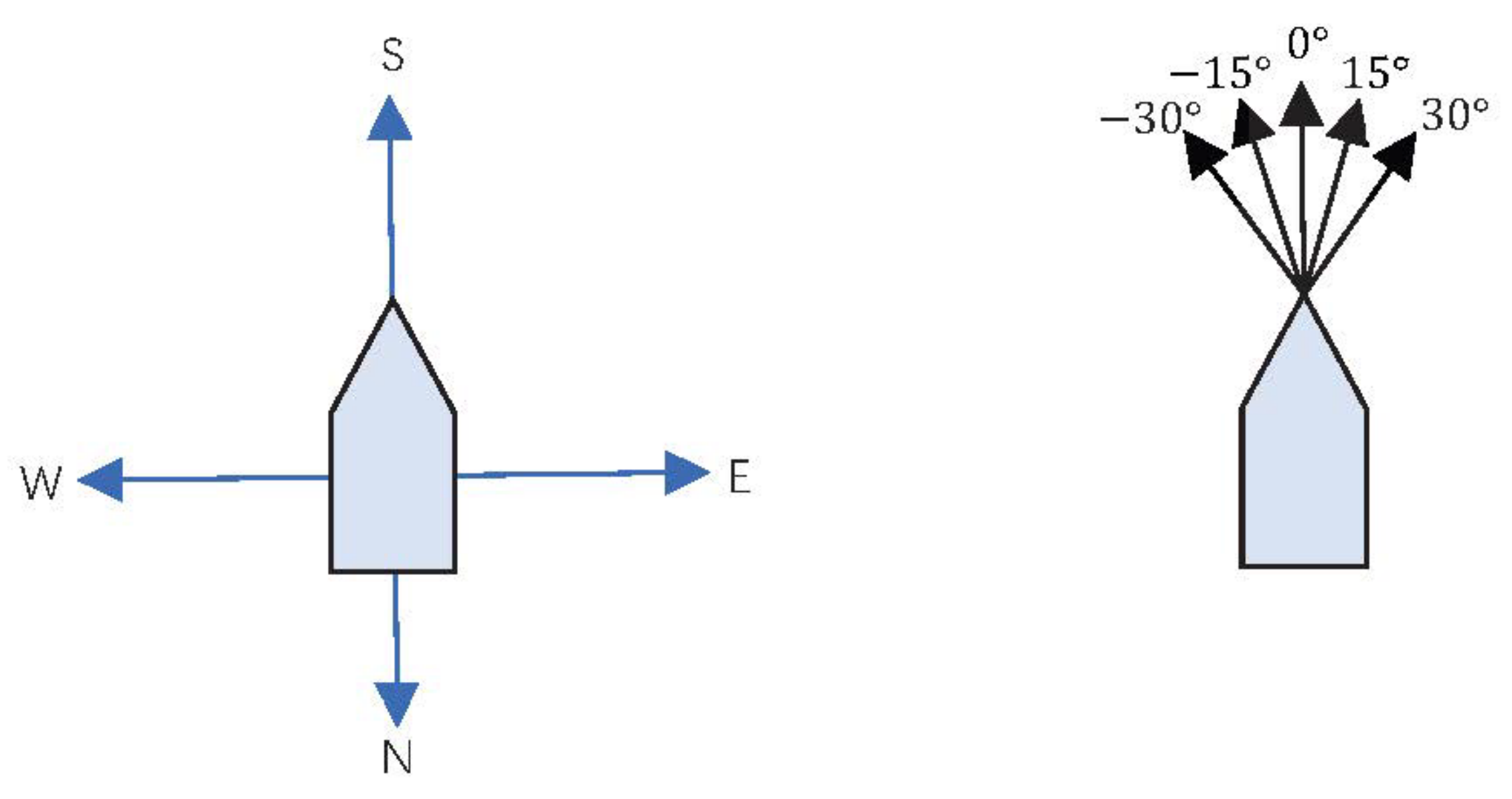
To align the turning angle of the unmanned boat with its actual navigation characteristics, the angle is crafted according to the principle of minimal-angle steering. The action space is defined to allow a single unit’s distance of advancement in a specified direction, with angles fixed at plus or minus 15 degrees, plus or minus 30 degrees, or 0 degrees.

Figure 3 illustrates this concept further, with the left diagram showing the action space as it is depicted in traditional reinforcement learning algorithms. The right diagram displays an optimized action space designed specifically to accommodate the operational attributes of the unmanned boat.

3.2. Environment Modeling

3.2.1. Environment Setting

In our simulation environment, we configure a map of dimensions 320 by 320, with the unmanned boat’s objective being to locate the most efficient route to a specific target point. We represent the state of the unmanned boat with the triplet $\left(x,y,\alpha \right)$, where $x$ and $y$ are the real-time coordinates of the boat within the simulated terrain, and $\alpha$ signifies the yaw angle relative to the target.

Starting from the initial coordinates of $\left(x_0,y_0\right)$, the actual heading angle is given by $\theta =\arctan \left(x_0,y_0\right)$. When considering the current coordinates as $\left(x,y\right)$ and the target coordinates as $\left(p,q\right)$, we can derive the desired heading through the following formula:

$$\beta =\arctan \left(x-p,y-q\right)-\arctan \left(x,y\right)$$

(16)

As the boat carries out actions from the set, each corresponding to a specific heading angle $a$, the actual heading angle changes accordingly. We can represent this as $a_{\theta }$, and update the heading angle with

$${\theta }_{\mathrm{new} }={\theta }_{\mathrm{old} }+a_{\theta }$$

(17)

The yaw angle $\alpha$ is then characterized as

$$\alpha =\beta -\theta$$

(18)

And the steering angle $\Delta \theta$ is determined as

$$\Delta \theta ={\theta }_{\mathrm{new} }-{\theta }_{\mathrm{old}}$$

(19)

3.2.2. Design of Reward Function

Proper reward configuration requires thoughtful consideration. If it is mishandled, an impractical reward scheme might lead to suboptimal results, which is even worse than a random strategy since it can incorrectly direct intelligent behavior. Typically, rewards are structured on a punitive basis until the objective is achieved, and these rules should not be overly complex. Therefore, a common reward scheme might consist of granting a significant bonus for meeting the goal and a minor penalty for failure to do so. To mitigate the drawbacks of sparse rewards, we have refined the incentives for the unmanned boat. The following outlines the guidelines for the interaction between the unmanned boat and its environment:

• Goal Achievement: A reward of +100 is given when the drone boat successfully reaches the final target. This substantial positive incentive is designed to guide the drone boat toward the target location;
• Collision Penalties: If the drone boat encounters an obstacle or boundary, it incurs a penalty of −2. Since these are undesired actions, the negative penalty encourages avoidance of these elements;
• Distance Rewards: The rewards are set at +1 or −1 depending on whether the drone boat’s distance to the target is decreasing or increasing, respectively. This drives the drone boat to approach the target while avoiding diverging from it;
• Yaw Angle Rewards: The smaller the yaw angle $\alpha$ of the drone boat, the higher the reward. This serves to push the drone boat to minimize the difference between its actual and desired heading, smoothing its path, averting unnecessary trajectories, and shortening the planned route;
• Steering Angle Rewards: Likewise, the more the steering angle $\Delta \theta$ of the unmanned boat is reduced, the greater the reward is given. This incentivizes the unmanned boat to curtail the steering angle, which in turn decreases the turning torque and the boat’s inclination on the water surface. As a result, this conserves energy, extends range, and diminishes the possibility of capsizing.

To align with points 4 and 5, we utilize the cosine of the corresponding angle as the reward. Also, when applying the memory playback mechanism, we aggregate the rewards for a sequence of states, eight in length, and assign it to this macro-action. Such an arrangement enables the Critic network to appraise the macro action as either positive or negative, augmenting the network’s discernment of different action sequence qualities. Consequently, the network’s proficiency in evaluating the merits of various action sequences is bolstered.

3.2.3. DDPG Based on USV Details

Actor Network Configuration: input layer: state size 19; hidden layer: 2 layers, 256 nodes per layer; output layer: actions of size 2. Critic Network Configuration: input Layer: total state and action size 20; hidden layer: 2 layers, 256 nodes per layer; output layer: 1 node; hyperparameters. Learning rate: 0.001, discount factor: 0.99, soft update rate ($\tau$): 0.005.

3.3. Design of Environment Settings and Reward Functions

In our simulation, a grid of 320 by 320 units will be employed, where each unit on the map signifies 5 m. And randomly designed obstacles on the map and indicated them with black squares on the map.The unmanned boat will traverse 5 units—or 25 m—in the direction of its current heading during each movement. This setup aims to curtail the amount of motion searches and expedite the algorithm’s validation. The training will be performed on the map 2000 times, with each iteration confined to 500 steps. If the final destination is not reached within those 500 steps, the attempt will be categorized as a failure.

The criteria for comparison include the mean number of steps taken, average rewards earned, success rate, overall path length, and the frequency of substantial-angle turns. To streamline the simulation process, obstacles have been shaped into rectangular forms. Moreover, we will establish a control group by constructing a conventional, fully connected neural network using the traditional Actor–Critic algorithm. To bolster the stability and efficiency of training, we will implement a Q target network to augment the convergence of iterations.

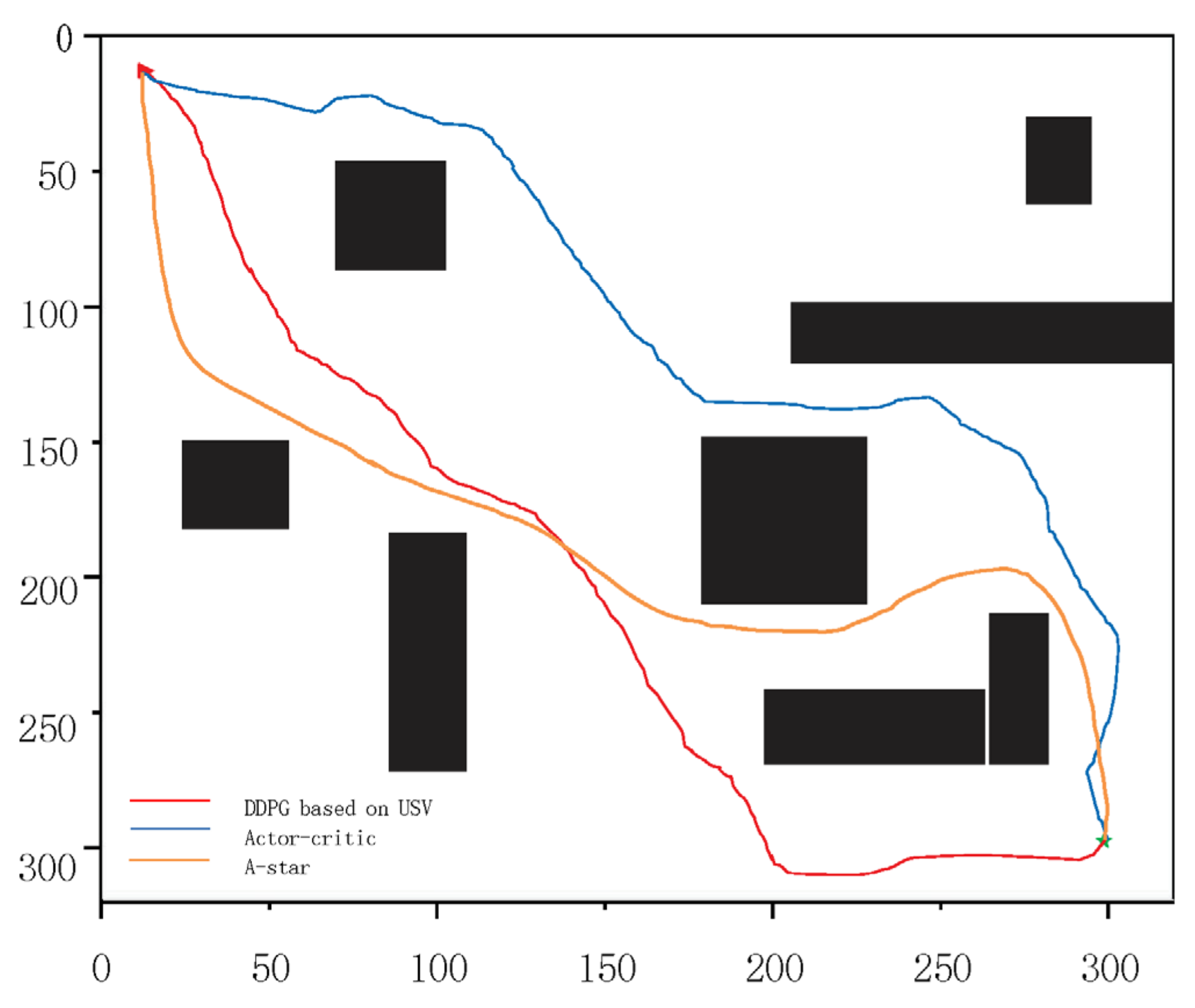
The visual representation of the simulation environment is as follows: obstacles are depicted as black rectangles, the starting point is marked by a red triangle, and the target point is symbolized by a green pentagram. After 2000 times of training, the path-planning trajectories for two algorithms are obtained. The red path illustrates the DDPG algorithm tailored for USV, while the blue path represents the Actor–Critic algorithm.

4. Discussion

Figure 4 depicts the simulation outcomes on the map, where the DDPG method adapted for USV clearly outperforms the traditional Actor–Critic algorithm. Specifically, the track length executed by the USV-focused DDPG is 2315.76 m, in contrast to the Actor–Critic algorithm’s track length of 2513.41 m; the track length executed by the A-star algorithm is 2607.93 m.

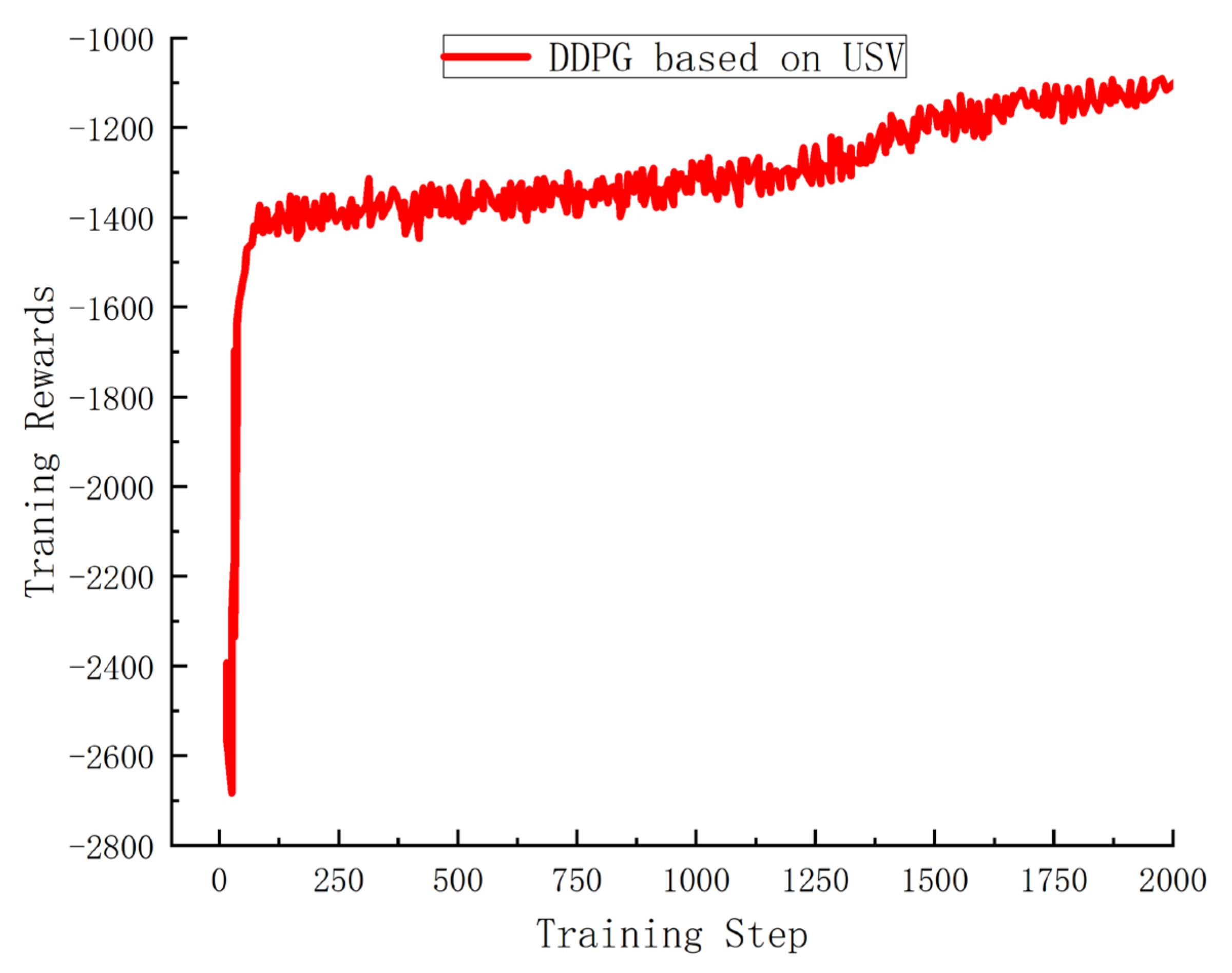
In Figure 5, the progression of reward alterations during USV’s training is demonstrated. In the graph, the X-axis signifies the count of training iterations (or episodes), while the Y-axis marks the total rewards accumulated by the drones in each round. By analyzing Figure 5, it is evident that as training advances, although the absolute rewards decline, the rewards themselves exhibit a gradual ascension, reflecting an overall convergence pattern.

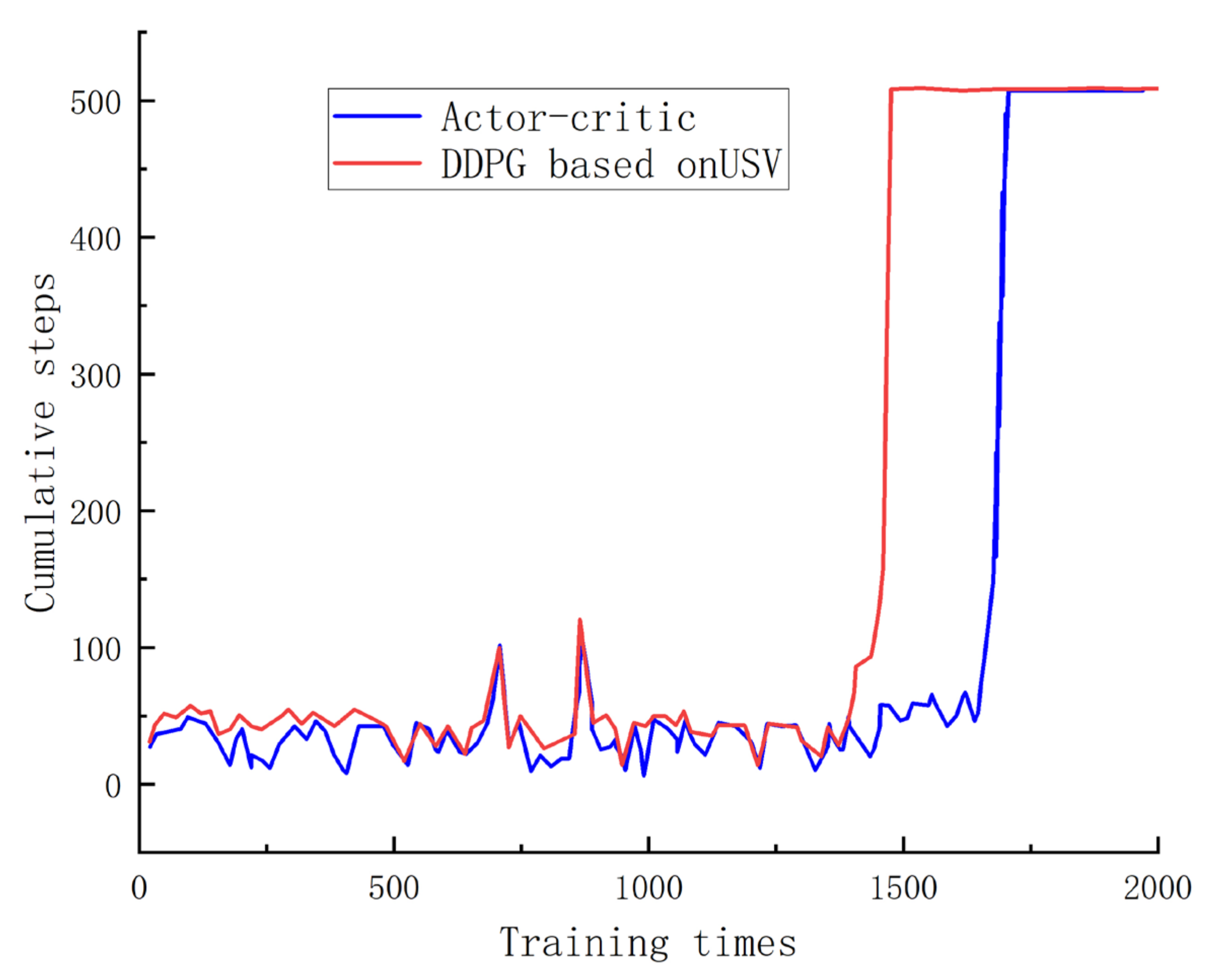
Figure 6 illustrates the correlation between the sum of training steps and cumulative step size. An examination of this figure reveals that the DDPG completes path planning sooner as the training steps are augmented, whereas the AC algorithm accomplishes it later. This pattern indicates superior convergence with the DDPG algorithm in comparison to the AC algorithm.

Table 4. Running results of each algorithm.

Simulation Algorithmic	Average Reward	Average Steps	Path Length	Number of Turns
DDPG based on USV	170.65	366.42	2315.76	3
Actor–Critic	163.70	432.78	2513.41	19
A-star	105.63	537.51	2607.93	6

provides statistical information gathered from the simulation experiments. From these data, it can be inferred that the average return of USV-focused DDPG training exceeds that of the traditional full Actor–Critic approach and far exceeds that of the A-star algorithm. In addition, the average number of steps is significantly reduced, the path lengths are shorter, and the frequency of turns is significantly reduced when training with DDPG compared to the paths generated by Actor–Critic as well as the paths generated by the A-star algorithm.

According to the above simulation results, it is obvious that the USV-based DDPG algorithm performs well on the path planning task. Its average reward is 170.65, which is significantly higher than the 163.70 of the Actor–Critic algorithm and 105.63 of the A-star algorithm, which indicates that the algorithm is more successful in selecting effective paths.

In addition, the USV-based DDPG algorithm also outperforms the other two algorithms in terms of the average number of steps, path length, and number of turns. Its average number of steps 366.42 is much less than Actor–Critic’s 432.78 and A-star’s 537.51, indicating that DDPG is more efficient in reaching its destination. Also, the DDPG algorithm has a shorter path length of 2315.76 than the other two algorithms, which indicates that it finds a more direct and optimized path. The most obvious is the number of turns, which is only 3 for DDPG compared to 19 for Actor–Critic and 6 for A-star. A lower number of turns means a smoother and more continuous path, which is very important for unmanned vessels in real-world applications, as too many turns may lead to increased energy consumption and navigation difficulties.

In summary, the USV-based DDPG algorithm excels in obtaining rewards and also outperforms other algorithms in terms of efficiency, path selection, and stability. These results strongly support the use of the DDPG algorithm in unmanned vessel path planning, especially in applications that require fast, efficient, and stable paths.

5. Conclusions

This study provides an in-depth comparison and analysis of the performance of multiple path planning algorithms, including USV-based DDPG, Actor–Critic, and A-star algorithms in a simulated environment. The data show that USV-based DDPG outperforms the other methods in terms of average reward, average number of steps, path length, and number of turns.

Firstly, USV-based DDPG shows significant improvement in average reward compared to other algorithms, which indicates its superior performance in path-planning tasks. Also, its average step count and path length are much lower than other algorithms, which indicates that it can find paths faster, and the paths that have been found are more concise and direct. In addition, USV-based DDPG makes far fewer turns than Actor–Critic, which further proves the efficiency and accuracy of its path planning.

Although the Actor–Critic and A-star algorithms also have their advantages in some aspects, the USV-based DDPG undoubtedly demonstrates its superiority in terms of overall performance. This may be attributed to its deep reinforcement learning nature and specific optimization of USV.

However, any research has its own limitations. In future work, further efforts shall be made to explore different model parameters and settings so that the performance of these algorithms in different contexts can be fully evaluated.

Overall, this study provides valuable insights into the comparison of path-planning algorithms in simulated environments and provides a solid foundation for future research and practical applications.