Insights into Bending Stiffness Modeling of Elementary Flexure Hinges

Abstract

Flexure hinges are widely used in mechanical devices, especially for micro- or even nano-scale applications, where conventional joints based on conjugate surfaces prove unsuitable. However, to achieve accurate motion of devices whose joints are flexure hinges, knowledge of stiffness models that correlate applied forces or bending moments with the resulting displacements is required. Nonlinear bending models are typically too complex and difficult to implement. Therefore, it is preferred to use linear models, which admit analytical solutions. The purpose of this paper is to show what is lost in terms of accuracy in reducing a nonlinear bending stiffness model associated with a flexure hinge when simplifications are made to obtain an analytical solution. An analysis of the simplification process leading to a linear stiffness model and its analytical solution is presented. From this study arises an increased awareness of flexure joints in terms of the accuracy obtained with their stiffness models, suggesting important information to the user in choosing the level of complexity required to model them in a specific application. A comparison between analytical and numerical results is provided in the form of maps and tables so as to make that choice as clear as possible.

1. Introduction

In traditional mechanics, mechanisms usually consist of rigid links connected by joints based on the principle of conjugate surfaces, typically lubricated and in sliding contact.

Recent research efforts have been directed toward designing mechanisms and mechanical systems at different scales, from macro to nano. However, they typically have some drawbacks, such as assembly, friction, and lubrication problems. Among the technical solutions proposed to overcome them, compliant mechanisms (CMs) have become increasingly popular in mechanical design, especially for micro and nano manipulators in the measurement industry. CMs are mechanisms in which conventional kinematic pairs are replaced by flexure hinges [1]. They have been extensively studied in the scientific literature, with examples in many fields of application and with different objectives: mechanisms featuring constant force [2] and multistable equilibrium [3], micro-electromechanical systems (MEMS) [4], positioning stages and precision grippers [5,6,7], micro/nano manipulators [8], fast servo tools for precision machining [9], servo valves [10] and other devices in the fields of energy harvesting [11], micro-vibration suppression [12], alignment of optics and robotic actuation [13], and many others.

In general, planar CMs have received more attention than their spatial counterparts. In fact, the former are more popular because they can be easily manufactured with EDM (Electrical Discharge Machining) technology. Moreover, their position kinematics can be more easily modeled, allowing for easier implementation in small-scale mechatronic systems that make use of flexures.

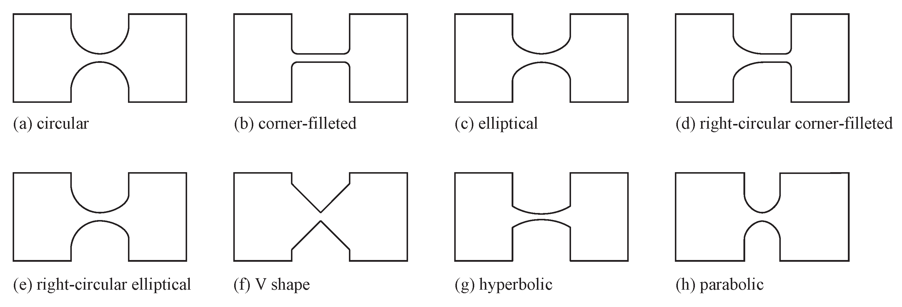
Many are the geometries of flexure hinges that have been studied: circular [14], elliptical [15], corner-filleted [16], parabolic and hyperbolic [17], cycloidal [18], filleted V-shaped [19], conical with a generalized model [20,21] and various hybrid flexure hinges [22,23]. Some of these geometries are shown in the chart of Figure 1.

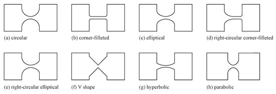
Figure 1. Chart of the most frequent geometries of flexures.

Many techniques and methods have been proposed to study various flexure hinges and compliant mechanisms, especially in the linear field. Some of them are based on elastic beam theory [24,25,26], some on stiffness and compliance matrices [27,28], some on elliptic integrals [29,30,31] and Castigliano’s theorem [17,23]. Ling et al. [32] proposed a classification of the various methods based on the objectives of the analysis at hand, such as the need for static or dynamic models of CMs [33,34,35]. The search for analytical models that describe the behavior of flexure hinges is of great use. In controllers of compliant mechanisms, easy-to-implement control logic based on kinematic models that are simple and quick to compute is required. Although finite element models typically provide more accurate solutions than analytical models, the former are usually implemented in dedicated simulation environments and require more computation time. In closed kinematic chain systems where there are many joints, it becomes crucial to have kinematic models of the whole mechanism that quickly and accurately provide the relation between the actuated joints and the end-effector operating in the mechanism workspace. Therefore, the simpler the model of the joint turns out to be, the simpler the model associated with the mechanism will be.

In the field literature, much more attention has been given to analyses of flexure hinges in small deformations. In contrast, only a small fraction of the papers have proposed studies on flexure hinges in large deformation [36,37,38,39,40].

In the present work, the bending of a flexure joint with a variable profile is modeled in large displacements by means of the Euler–Bernoulli beam Elastica Theory [41]. Some simplifications are applied to the nonlinear model to arrive at a model that can be solved in analytical form. The simplification process is described in detail to understand what is neglected in the process of obtaining an analytical solution and what it entails. In fact, each simplification step results in a loss of accuracy of the stiffness model used for the flexure joint. In this work, an analytical solution is first found for a flexure with any profile. Then, this solution is applied to a flexure hinge with a rectangular section and an elliptical profile. An extension to other geometries is quite straightforward. Toward the end of the paper, a comparison is made between the results of the analytical solution of the simplified model and the numerical solution of the complete nonlinear model. The results are proposed in the form of maps and tables to appreciate the effect of varying different parameters on the accuracy of the stiffness model chosen for the flexure joint of interest. An example of how to use the information reported in this paper is shown in [42], where a case study is proposed to provide instructions for designing a flexure hinge with given specifications.

2. Nonlinear Bending of a Straight Beam

2.1. Large Displacement Model of a Planar Beam

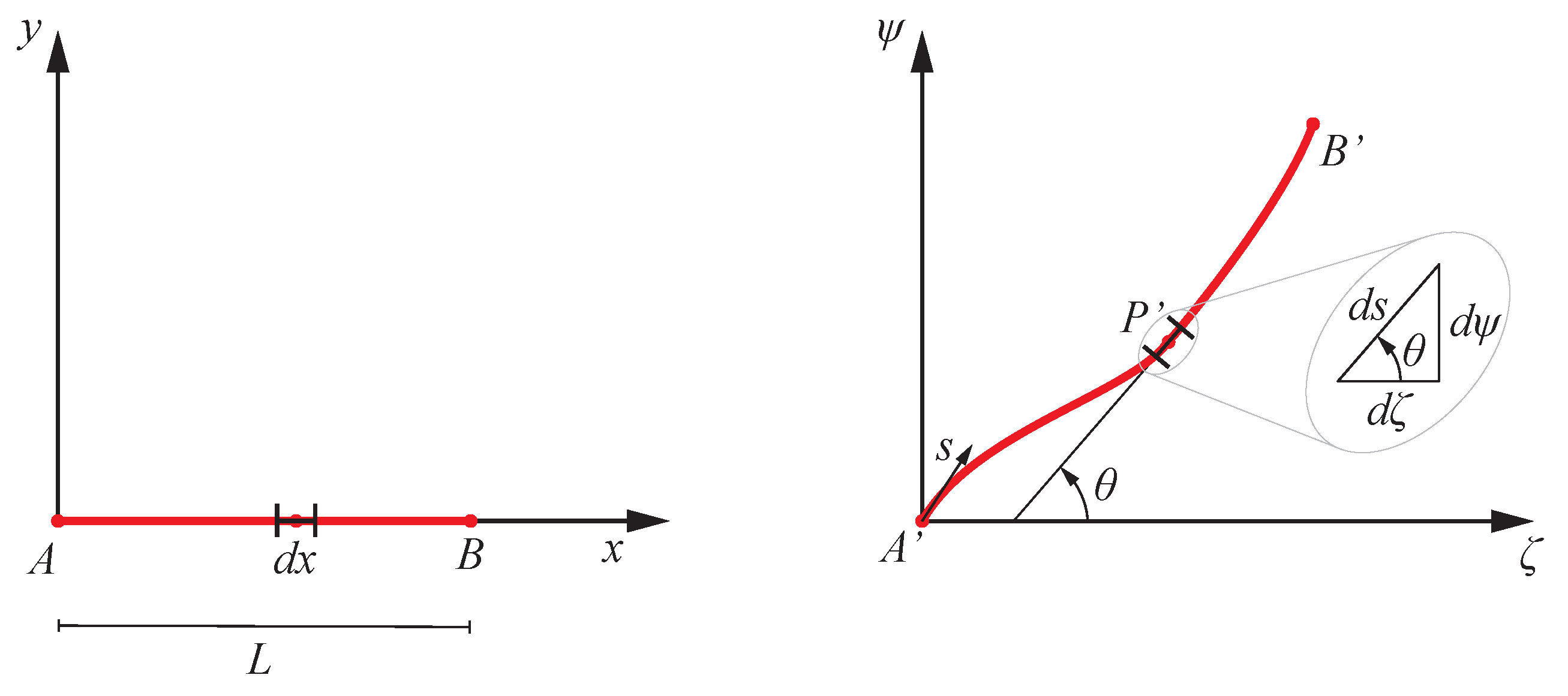
This work starts from a straight axis Euler–Bernoulli beam of length L in the plane $xy$, as shown in Figure 2 on the left, aligned with the x-axis. It follows that all results shown below refer to beams that meet the assumptions of Euler–Bernoulli’s model. Furthermore, the study of flexures characterized by homogeneous and isotropic material under nominal temperature conditions is addressed.

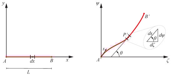
Figure 2. Undeformed and deformed states of a straight axis beam (left) and load conditions (right).

The undeformed state of the beam represents the reference condition, with points A and B being its two ends. Under static loads acting on the mentioned plane the beam changes geometry and assumes a different shape, where the new positions $A^{\prime }$ and $B^{\prime }$ of its extremes result in accordance with the planar load condition shown in Figure 3, namely a force $R_0$ in a generic direction of the plane $xy$ and a bending moment $M_f$ about its orthogonal z-axis applied at point B, or more generally at point $B^{\prime }$ after the beam deformation.

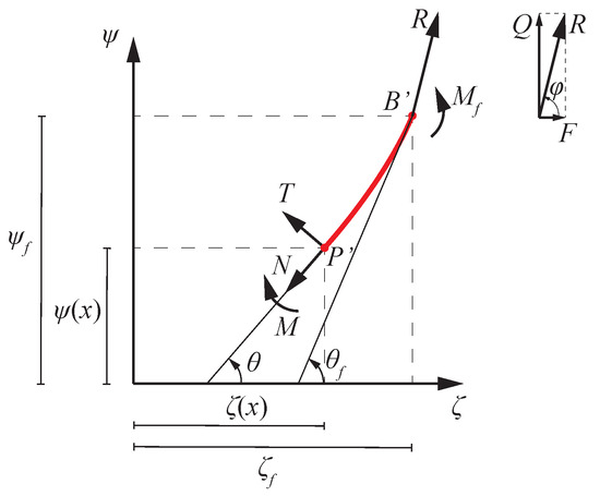
Figure 3. Static load conditions.

A generic infinitesimal element $dx$ in the beam reference condition deforms into the element $ds$, which assumes the new coordinate position $\zeta$ and $\psi$. The two differentials $dx$ and $ds$ are related by the following relationship: $ds=dx(1+\epsilon )$, where $\epsilon$ is the axial deformation of the beam.

Be M the axial bending moment, E the Young’s modulus, $I_z$ the moment of inertia of the beam section, and $\kappa$ the beam curvature. Two definitions of curvature can be found in the literature: the mechanical curvature and the geometric curvature, denoted as ${\kappa }_m$ and ${\kappa }_g$ respectively [43]:

$$\begin{array}{c}{\kappa }_m={\displaystyle \frac{d\theta }{dx}}\hfill \\ {\kappa }_g={\displaystyle \frac{d\theta }{ds}}={\displaystyle \frac{d\theta }{dx}}{\displaystyle \frac{dx}{ds}}={\displaystyle \frac{{\kappa }_m}{1+\epsilon }}\hfill \end{array}.$$

(1)

In the scientific literature, ${\kappa }_m$ is commonly used [44,45,46] for many reasons, in particular for its simplicity and its feature of isolating the effect of pure bending from curvature variations produced by stretching. However, in other works [47,48,49] ${\kappa }_g$ is preferred over ${\kappa }_m$ because it is considered the most correct curvature due to its geometric meaning.

With reference to Figure 3, a static analysis of a portion of the beam, from the generic section $P^{\prime }$ to its end $B^{\prime }$ where external loads are applied, provides the moment equation with respect to $ds$ or $dx$:

$$\begin{array}{c}{\displaystyle \frac{dM}{ds}}=R_{0}sin\left(\theta -\phi \right)\hfill \\ {\displaystyle \frac{dM}{dx}}=\left(1+\epsilon \right)R_{0}sin\left(\theta -\phi \right)\hfill \end{array},$$

(2)

where $\phi$ is the slope of vector R of magnitude $R_0$ with respect to the x-axis.

Exploiting the curvature-moment relationship and the definition of curvature, the following differential equations can be found:

$$\begin{array}{cc}{\theta }^{″}\left(x\right)+\frac{I_z^{\prime }\left(x\right)}{I_z\left(x\right)}{\theta }^{\prime }\left(x\right)=\frac{R_0}{E{I}_z\left(x\right)}\left[1+\epsilon \left(x\right)\right]sin\left[\theta \left(x\right)-\phi \right]\hfill & \left(\kappa ={\kappa }_m\right)\hfill \\ {\theta }^{″}\left(x\right)+\left[\frac{I_z^{\prime }\left(x\right)}{I_z\left(x\right)}-\frac{{\epsilon }^{\prime }\left(x\right)}{1+\epsilon \left(x\right)}\right]{\theta }^{\prime }\left(x\right)={\frac{R_0}{E{I}_z\left(x\right)}\left[1+\epsilon \left(x\right)\right]}^{2}sin\left[\theta \left(x\right)-\phi \right]\hfill & \left(\kappa ={\kappa }_g\right)\hfill \end{array}$$

(3)

With the assumption of an inextensible beam, the axial deformation $\epsilon$ is negligible. Therefore, ${\kappa }_m={\kappa }_g={\theta }^{\prime }\left(x\right)$ and both equations in Equation (3) become the following reference equation:

$${\theta }^{″}\left(x\right)+\frac{I_z^{\prime }\left(x\right)}{I_z\left(x\right)}{\theta }^{\prime }\left(x\right)=\frac{R_0}{E{I}_z\left(x\right)}sin\left[\theta \left(x\right)-\phi \right]$$

(4)

2.2. Dimensionless Model of a Planar Beam

Equation (4) is a nonlinear differential equation with variable coefficients and can only be solved numerically. The search for an analytical solution is only possible if some of its terms are negligible. It follows that a comparison regarding the relevance of each term of the differential equation is required.

In order to highlight and compare the weight of the various terms that multiply $\theta \left(x\right)$ and its derivatives, Equation (4) can be made dimensionless. This processing has the ultimate goal of simplifying the lower-order terms and subsequently seeking an analytical solution when available. Therefore, it is assumed that:

$$\begin{array}{c}x=x_0\tilde{x}\hfill \\ I_z=I_z\left(x\right)=I_z\left[x\left(\tilde{x}\right)\right]={\overline{I}}_z\left(\tilde{x}\right)=I_{z0}{\tilde{I}}_z\hfill \end{array},$$

(5)

where $x_0$ is the dimensional part of x, whereas $\tilde{x}$ is its dimensionless part. Similarly for $I_{z0}$ and ${\tilde{I}}_z$. Moreover, $\epsilon \left(x\right)$ and $\theta \left(x\right)$ in Equation (4) are dimensionless as well by definition, with $\epsilon \left(x\right)=\tilde{\epsilon }\left(\tilde{x}\right)$ and $\theta \left(x\right)=\tilde{\theta }\left(\tilde{x}\right)$.

In accordance with the previous relations and by means of their substitution in Equation (4), a dimensionless form of the equation can be written as:

$${\tilde{\theta }}^{″}\left(\tilde{x}\right)+\frac{{\tilde{I}}_z^{\prime }\left(\tilde{x}\right)}{{\tilde{I}}_z\left(\tilde{x}\right)}{\tilde{\theta }}^{\prime }\left(\tilde{x}\right)=\frac{R_0{x}_0^2}{E{I}_{z0}{\tilde{I}}_z\left(\tilde{x}\right)}sin\left[\tilde{\theta }\left(\tilde{x}\right)-\phi \right].$$

(6)

3. Analytical Solution of the Flexure Joint Bending Stiffness Model

3.1. Nonlinear Model Simplification and Analytical Solution

If steel is taken as reference material, it can be assumed that the maximum rotation $\theta$ will always be confined below the maximum rotation at the yield strength in order to avoid permanent shape deformations. This means that the sine function in Equation (6) can be expanded in Taylor series, namely:

$$sin\left[\tilde{\theta }\left(\tilde{x}\right)-\phi \right]\approx cos\left(\phi \right)\tilde{\theta }\left(\tilde{x}\right)-sin\left(\phi \right),$$

(7)

On the basis of all these assumptions, the following simplified form is obtained:

$${\tilde{\theta }}^{″}\left(\tilde{x}\right)+\frac{{\tilde{I}}_z^{\prime }\left(\tilde{x}\right)}{{\tilde{I}}_z\left(\tilde{x}\right)}{\tilde{\theta }}^{\prime }\left(\tilde{x}\right)+a\left(\tilde{x}\right)\tilde{\theta }\left(\tilde{x}\right)=b\left(\tilde{x}\right),$$

(8)

where

$$\begin{array}{c}a\left(\tilde{x}\right)=-{\displaystyle \frac{A{x}_0^2}{E{I}_{z0}{\tilde{I}}_z\left(\tilde{x}\right)}}cos\left(\phi \right)\hfill \\ b\left(\tilde{x}\right)=-{\displaystyle \frac{A{x}_0^2}{E{I}_{z0}{\tilde{I}}_z\left(\tilde{x}\right)}}sin\left(\phi \right)\hfill \end{array}.$$

(9)

An equation with variable coefficients, such as Equation (8), admits an analytical solution when the zero-order derivative term is identically null. Therefore, on a preliminary basis it is assumed that the maximum value of $\left|a\left(\tilde{x}\right)\right|$ is small and negligible when compared to the coefficients of the other terms in Equation (8), namely “1” and $\left|\frac{{\tilde{I}}_z^{\prime }\left(\tilde{x}\right)}{{\tilde{I}}_z\left(\tilde{x}\right)}\right|$ for the second- and first-order derivatives respectively.

It should be noted that $\left|a\left(\tilde{x}\right)\right|$ and $\left|b\left(\tilde{x}\right)\right|$ differ only for their sinusoidal term, namely $sin\left(\phi \right)$ and $cos\left(\phi \right)$ respectively. If $sin\left(\phi \right)\le cos\left(\phi \right)$, then coefficient $\left|b\left(\tilde{x}\right)\right|$ should be neglected as well. However, the presence of the term $b\left(\tilde{x}\right)$ does not affect the existence or non-existence of the analytical solution. On the contrary, it only improves its quality. Therefore, it will be considered, regardless of the value of the angle $\phi$.

Finally, a further simplified version of Equation (8) is obtained:

$${\tilde{\theta }}^{″}\left(\tilde{x}\right)+\frac{{\tilde{I}}_z^{\prime }\left(\tilde{x}\right)}{{\tilde{I}}_z\left(\tilde{x}\right)}{\tilde{\theta }}^{\prime }\left(\tilde{x}\right)=b\left(\tilde{x}\right),$$

(10)

whose domain and validity have to be verified in order to be considered acceptable, as shown in the following.

Finally, the analytical solution can be made explicit, bearing in mind that it relates to a simpler model than the complete nonlinear one given in Equation (6). In fact, the solution of Equation (10) has the following form:

$$\tilde{\theta }\left(\tilde{x}\right)={\int }_{{\tilde{x}}_i}^{\tilde{x}}\frac{c_1+c_2\tau }{{\tilde{I}}_z\left(\tau \right)}d\tau ,$$

(11)

where ${\tilde{x}}_i$ and $c_1$ are coefficients that result from two boundary conditions applied to Equation (10) related to the beam constraints, whereas $c_2$ is:

$$c_2=b\left(\tilde{x}\right){\tilde{I}}_z\left(\tilde{x}\right)=-{\displaystyle \frac{A{x}_0^{2}sin\left(\phi \right)}{E{I}_{z0}}}.$$

(12)

3.2. Boundary Conditions

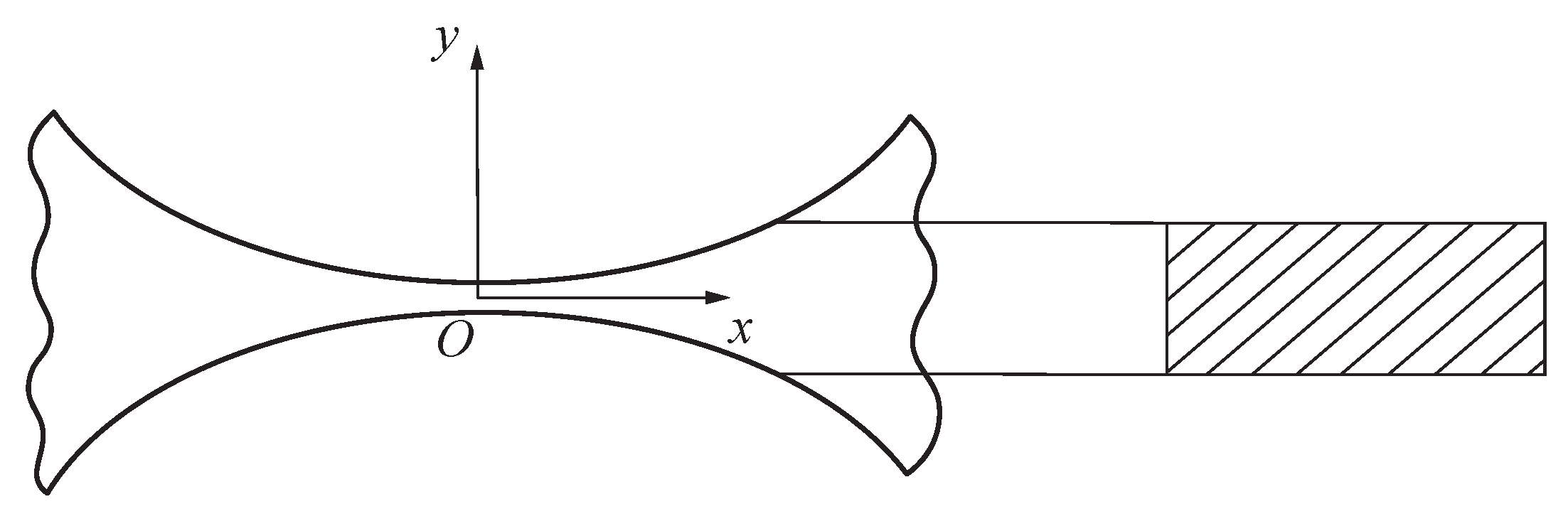
A beam with a generic double symmetric profile along the axis direction x and a cross-section with a rectangular shape in the $yz$ plane is considered.

A natural consequence of such a choice is considering elastic deformations only within the $xy$ plane. Given the double symmetry of the beam profile along its axis, it is convenient to place a reference system in the center of symmetry, as shown in Figure 4. It follows that $\tilde{x}\in \left[-1;1\right]$.

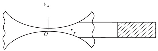
Figure 4. Beam geometry and local reference frame.

In order to study Equation (10), boundary conditions must be imposed. The study case of a beam fixed at one end and free to move at the other end is proposed. These two conditions are summarized as:

$$\begin{array}{c}\tilde{\theta }\left(-1\right)=0\hfill \\ {\tilde{\theta }}^{\prime }\left(1\right)={\displaystyle \frac{x_0{M}_0\tilde{M}\left(1\right)}{E{I}_{z0}{\tilde{I}}_z\left(1\right)}}\hfill \end{array},$$

(13)

where the second relation is obtained by applying a bending moment $M\left(x\right)=E{I}_z\left(x\right)\kappa \left(x\right)$ with $M\left(x\right)=M_0\tilde{M}\left(\tilde{x}\right)$. From Equations (11) and (13), the analytical solution of a beam subjected to static loads is obtained:

$$\tilde{\theta }\left(\tilde{x}\right)={\int }_{-1}^{\tilde{x}}\left[\frac{x_0{M}_0\tilde{M}\left(1\right)}{E{I}_{z0}{\tilde{I}}_z\left(\tau \right)}+c_2\frac{\tau -1}{{\tilde{I}}_z\left(\tau \right)}\right]d\tau .$$

(14)

4. Bending Stiffness Model of a Flexure Hinge

A simple bending stiffness model of a flexure hinge with a generic profile along its axis is useful when it is part of a more complex mechatronic device, and a user needs information about the driving forces or bending moments responsible for a desired kinematic behavior.

A relation between the maximum angular displacement and the known acting loads in terms of a stiffness coefficient can be derived from Equation (14) after small arrangements. The angular displacement of the joint is evaluated in $\tilde{x}=1$, and the moment applied to the free end of the beam is highlighted, leading to:

$$M_f=K{\theta }_f+\Delta M,$$

(15)

where

$$\begin{array}{ccc}{M}_f=M_0\tilde{M}\left(1\right),\hfill & & {\theta }_f=\tilde{\theta }\left(1\right),\hfill \\ K={\displaystyle \frac{1}{{\displaystyle {\int }_{-1}^1{\displaystyle \frac{x_0}{E{I}_{z0}{\tilde{I}}_z\left(\tau \right)}}d\tau }}},\hfill & & \Delta M={\displaystyle \frac{{\displaystyle c_2{\int }_{-1}^1{\displaystyle \frac{\left(1-\tau \right)}{{\tilde{I}}_z\left(\tau \right)}}d\tau }}{{\displaystyle {\int }_{-1}^1{\displaystyle \frac{x_0}{E{I}_{z0}{\tilde{I}}_z\left(\tau \right)}}d\tau }}}.\hfill \end{array}$$

(16)

Coefficients K and $\Delta M$ depend on the geometry of the beam, its material, and the amplitude of loads and moments applied to its free end.

In summary, several assumptions have been made to simplify both the differential equations in Equation (3) leading to Equation (10). Finally, the latter can be solved analytically. This simplification process has led toward a linearization of the nonlinear model, and, in addition, it allows us to understand under which conditions the solution of the linear problem is valid. Such a linear solution is formally the same as that proposed by Chen et al. [50] for an elliptic flexure. In the following section, a more detailed investigation of the conditions of validity of the linear analytical solution for an elliptic flexure is proposed.

4.1. Case Study: An Elliptical Flexure Hinge

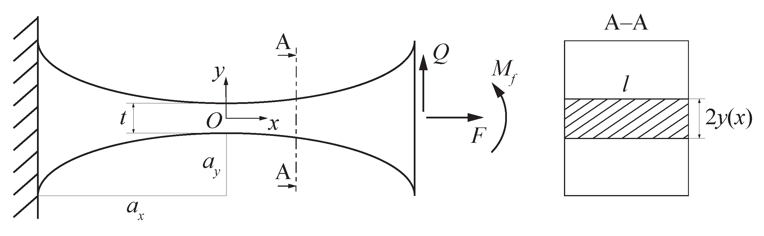
An example of the application of the model shown in the previous sections allows us to deepen the study in a real physical case. A flexure with a rectangular section and an elliptical profile under static loads is proposed as a case study, as shown in Figure 5. The cross-section of the flexure hinge changes its dimension with x; in fact, even if its horizontal side l is constant, its height is variable according to $2y\left(x\right)$. The smallest section in $x=0$ has a thickness of t. The major and minor semi-axes of the ellipsis in Figure 5 are $a_x$ and $a_y$, respectively.

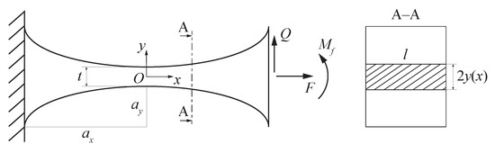
Figure 5. Elliptical flexure hinge with applied static loads.

The choice of elliptical geometry allows us to give an expression to the dimensional coefficients in Equation (5), namely $x_0$ and $I_{z0}$. The former can be easily identified, in fact:

$$x=a_x\tilde{x}\mathrm{with}\tilde{x}\in \left[-1;1\right].$$

(17)

The latter requires more processing, following a sequence of logical steps. It starts from the expression of an elliptical profile, as shown in [15]:

$$y\left(x\right)=a_y\left[\left(1+{\beta }_y\right)-\sqrt{1-{\left(\frac{x}{a_x}\right)}^2}\right].$$

(18)

Then, Equation (18) is converted into a new function of $\tilde{x}$ by means of Equation (17):

$$\overline{y}\left(\tilde{x}\right)=a_y\left[\left(1+{\beta }_y\right)-\sqrt{1-{\tilde{x}}^2}\right]=y_0\tilde{y}\left(\tilde{x}\right),$$

(19)

where

$$\begin{array}{ccc}{\beta }_y={\displaystyle \frac{t}{2a_y}};\hfill & y_0=a_y;& \hfill \tilde{y}\left(\tilde{x}\right)=\left(1+{\beta }_y\right)-\sqrt{1-{\tilde{x}}^2}\end{array}.$$

(20)

In Equation (19) $\tilde{y}\left(\tilde{x}\right)$ is the positive dimensionless y coordinate of the elliptical profile. Finally, said $I_z\left(x\right)=\frac{l{\left[2y\left(x\right)\right]}^3}{12}$ the moment of inertia of the cross section about the z-axis, which varies with x, and using both Equations (18) and (19), it follows the required expression of $I_{z0}$ and ${\tilde{I}}_z\left(\tilde{x}\right)$. Their product provides ${\overline{I}}_z\left(\tilde{x}\right)$ according to Equation (5):

$$\begin{array}{cc}{I}_{z0}={\displaystyle \frac{2}{3}}l{a}_y^3;\hfill & \hfill {\tilde{I}}_z\left(\tilde{x}\right)={\left[\left(1+{\beta }_y\right)-\sqrt{1-{\tilde{x}}^2}\right]}^3={\left[\tilde{y}\left(\tilde{x}\right)\right]}^3\end{array}.$$

(21)

4.2. Conditions of Applicability of the Linear Model

Once the profile of the flexure hinge is known, the applicability of the analytical model provided in Equation (14) can be verified by looking at the coefficient $a\left(\tilde{x}\right)$. An analysis of this term means understanding under which conditions the assumptions of its negligibility can be considered valid, namely when:

$$\begin{array}{c}\underset{\tilde{x}\in \left[-1;1\right]}{max}\left|a\left(\tilde{x}\right)\right|\ll 1\hfill \\ \underset{\tilde{x}\in \left[-1;1\right]}{max}\left|a\left(\tilde{x}\right)\right|\ll \underset{\tilde{x}\in \left[-1;1\right]}{min}\left|{\displaystyle \frac{{\tilde{I}}_z^{\prime }\left(\tilde{x}\right)}{{\tilde{I}}_z\left(\tilde{x}\right)}}\right|\hfill \end{array}.$$

(22)

From the first of Equation (22) it is:

$$\frac{a_x^2}{E{I}_{z0}}\frac{\left|F\right|}{\underset{\tilde{x}\in \left[-1;1\right]}{min}{\tilde{I}}_z\left(\tilde{x}\right)}\ll 1.$$

(23)

It is easy to verify that $\underset{\tilde{x}\in \left[-1;1\right]}{min}{\tilde{I}}_z\left(\tilde{x}\right)={\tilde{I}}_z\left(0\right)={{\beta }_y}^3$ by looking at the expression of the terms involved. A convenient substitution in Equation (23) can be made by introducing the following dimensionless parameters, as in [15]:

$$\begin{array}{cc}\rho ={\displaystyle \frac{a_x}{a_y}};\hfill & {\mu }_F={\displaystyle \frac{F}{El{a}_x}}\end{array}.$$

(24)

The first indicates how far the elliptical profile deviates from a circular profile, represented by $\rho =1$. The second allows the value of the axial force to be dimensionless.

Taking advantage of expressions in Equations (20) and (24), from Equation (23) the following condition on ${\mu }_F$ can be easily found:

$$|{\mu }_F|\ll \frac{2}{3}{\left({\displaystyle \frac{{\beta }_y}{\rho }}\right)}^3.$$

(25)

The second condition in Equation (22) can be re-elaborated as follows:

$$\frac{3}{2}{\left(\frac{\rho }{{\beta }_y}\right)}^3\left|{\mu }_F\right|\ll \underset{\tilde{x}\in \left[-1;1\right]}{min}\left|{\displaystyle \frac{{\tilde{I}}_z^{\prime }\left(\tilde{x}\right)}{{\tilde{I}}_z\left(\tilde{x}\right)}}\right|.$$

(26)

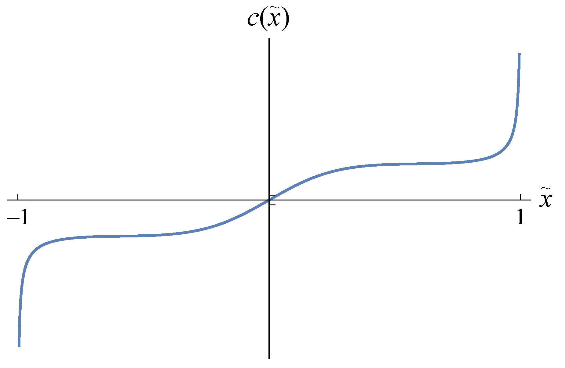
Said $c\left(\tilde{x}\right)=\frac{{\tilde{I}}_z^{\prime }\left(\tilde{x}\right)}{{\tilde{I}}_z\left(\tilde{x}\right)}$, its trend with a single zero in $\tilde{x}=0$, due to the fact that it is an odd function as it will be shortly demonstrated, can be observed in Figure 6. It follows that:

$$\underset{\tilde{x}\in \left[-1;1\right]}{min}\left|\frac{{\tilde{I}}_z^{\prime }\left(\tilde{x}\right)}{{\tilde{I}}_z\left(\tilde{x}\right)}\right|=0.$$

(27)

Figure 6. Trend of function $c\left(\tilde{x}\right)$.

The result just obtained demonstrates that there is certainly a range of $\tilde{x}$ in which the condition in Equation (26) is not verified. What follows is dedicated to finding the limits of this range.

A look at the expressions in Equation (21) reveals that $\widetilde{I_z}\left(\tilde{x}\right)$ is positive for $\tilde{x}\in [-1;1]$ with ${\beta }_y\in \left]0;1\right]$ and that it is an even function, namely $\widetilde{I_z}(-\tilde{x})=\widetilde{I_z}\left(\tilde{x}\right)$. Furthermore, its derivative is an odd function, namely $-{\widetilde{I_z}}^{\prime }(-\tilde{x})={\widetilde{I_z}}^{\prime }\left(\tilde{x}\right)$ or also ${\widetilde{I_z}}^{\prime }(-\tilde{x})=-{\widetilde{I_z}}^{\prime }\left(\tilde{x}\right)$.

It follows that $c\left(\tilde{x}\right)$ is an odd function, as mentioned above:

$$c(-\tilde{x})=\frac{{\widetilde{I_z}}^{\prime }\left(\widetilde{-x}\right)}{\widetilde{I_z}\left(\widetilde{-x}\right)}=-\frac{{\widetilde{I_z}}^{\prime }\left(\tilde{x}\right)}{\widetilde{I_z}\left(\tilde{x}\right)}=-c\left(\tilde{x}\right).$$

(28)

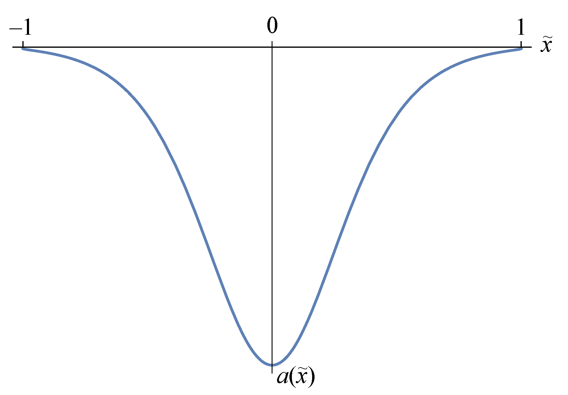
A similar analysis can be addressed for $a\left(\tilde{x}\right)$. According to Equation (9), it is easy to verify that it is an even function, in fact:

$$a(-\tilde{x})=-\frac{A{a}_x^{2}cos(\phi )}{E{I}_{z0}}\frac{1}{{\tilde{I}}_z(-\tilde{x})}=-\frac{A{a}_x^{2}cos\left(\phi \right)}{E{I}_{z0}}\frac{1}{{\tilde{I}}_z\left(\tilde{x}\right)}=a\left(\tilde{x}\right).$$

(29)

Its sign depends on the sign of $cos\left(\phi \right)$. Assuming that the latter is positive, it follows that $a\left(\tilde{x}\right)<0$ for $\tilde{x}\in \left[-1;1\right]$, as shown in Figure 7, whereas $c\left(\tilde{x}\right)\le 0$ for $\tilde{x}\in \left]-1;0\right]$. Therefore, the two functions $a\left(\tilde{x}\right)$ and $c\left(\tilde{x}\right)$ may intersect only within the range $\left]-1;0\right]$ of $\tilde{x}$, as shown in Figure 8. It follows that $a\left(\tilde{x}\right)$ is certainly smaller than $c\left(\tilde{x}\right)$ for $\tilde{x}\in \left[0;{\tilde{x}}_z\right]$.

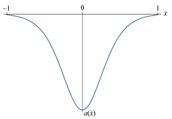
Figure 7. Trend of function $a\left(\tilde{x}\right)$ when $cos\left(\phi \right)>0$.

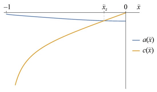
Figure 8. Intersection between functions $a\left(\tilde{x}\right)$ and $c\left(\tilde{x}\right)$.

A deeper investigation is needed for $\tilde{x}\in \left[-1;0\right]$. A difference function can be defined as:

$$d\left(\tilde{x}\right)=c\left(\tilde{x}\right)-a\left(\tilde{x}\right).$$

(30)

An analytical study of Equation (30) to find its zeros is too complex because it requires a sixth-degree polynomial to be solved. Under condition Equation (25), a linear approximation of Equation (30) by means of a Taylor series and a subsequent search for its zero provides:

$${\tilde{x}}_z=-\frac{{\beta }_y}{2}{\left(\frac{\rho }{{\beta }_y}\right)}^3{\mu }_F.$$

(31)

Therefore, in the range $-1\le \tilde{x}\le 0$ the condition $\left|a\left(\tilde{x}\right)\right|<\left|c\left(\tilde{x}\right)\right|$ is met when $-1\le \tilde{x}<{\tilde{x}}_z$. The property of symmetry of both functions $\left|a\left(\tilde{x}\right)\right|$ and $\left|c\left(\tilde{x}\right)\right|$ allows to state that:

$$\left|a\left(\tilde{x}\right)\right|<\left|c\left(\tilde{x}\right)\right|\mathrm{for}\tilde{x}\in \left[-1;{\tilde{x}}_z\right[\wedge \left]{-\tilde{x}}_z;1\right].$$

(32)

Since it is required that $|{\tilde{x}}_z|<<1$, the following relationship must hold:

$$|{\mu }_F|\ll \frac{2}{{\beta }_y}{\left({\displaystyle \frac{{\beta }_y}{\rho }}\right)}^3.$$

(33)

Comparing conditions in Equations (25) and (33) it turns out that:

$$\left[\frac{2}{3}{\left(\frac{{\beta }_y}{\rho }\right)}^3\right]/\left[\frac{2}{{\beta }_y}{\left(\frac{{\beta }_y}{\rho }\right)}^3\right]=\frac{{\beta }_y}{3}<1;$$

(34)

therefore the condition in Equation (25) is more restrictive than the one in Equation (33). Furthermore, the average values of $a\left(\tilde{x}\right)$ and $c\left(\tilde{x}\right)$ in the range $\left[-1;0\right]$ of $\tilde{x}$ (or $\tilde{x}\in \left[0;1\right]$ when $cos\left(\phi \right)<0$) are:

$$\begin{gathered} \begin{array}{c}|\overline{a\left(\tilde{x}\right)}|={\displaystyle \frac{3\left[3\pi {\delta }_y^2+6\sqrt{{\beta }_y{\gamma }_y}+8\sqrt{{\beta }_y^3{\gamma }_y}+4\sqrt{{\beta }_y^5{\gamma }_y}+6{\delta }_y^2{tan}^{-1}\left({\displaystyle \frac{1}{\sqrt{{\beta }_y{\gamma }_y}}}\right)\right]}{8{\delta }_y{\left({\beta }_y{\gamma }_y\right)}^{\frac{5}{2}}}}{\rho }^3|{\mu }_F|\\ \\ |\overline{c\left(\tilde{x}\right)}|=-3ln\left({\displaystyle \frac{{\beta }_y}{{\delta }_y}}\right)\end{array}, \end{gathered}$$

(35)

where ${\delta }_y=1+{\beta }_y$ and ${\gamma }_y=2+{\beta }_y$. Pursuing the goal of having $|\overline{a\left(\tilde{x}\right)}|<<|\overline{c\left(\tilde{x}\right)}|$, it follows that:

$$|{\mu }_F|<<{\displaystyle \frac{8{\delta }_y{\left({\beta }_y{\gamma }_y\right)}^{\frac{5}{2}}}{3\left[-3\pi {\delta }_y^2-6\sqrt{{\beta }_y{\gamma }_y}-8\sqrt{{\beta }_y^3{\gamma }_y}-4\sqrt{{\beta }_y^5{\gamma }_y}-6{\delta }_y^2{tan}^{-1}\left({\displaystyle \frac{1}{\sqrt{{\beta }_y{\gamma }_y}}}\right)\right]}}\frac{1}{{\rho }^3}.$$

(36)

It is easy to verify that the condition in Equation (25) is more restrictive than the one in Equation (36) for any ${\beta }_y\in \left]0;1\right]$. Under the constraint in Equation (25) the condition $\underset{\tilde{x}\in \left[-1;1\right]}{max}\left|a\left(\tilde{x}\right)\right|\ll \underset{\tilde{x}\in \left[-1;1\right]}{min}\left|\frac{{\tilde{I}}_z^{\prime }\left(\tilde{x}\right)}{{\tilde{I}}_z\left(\tilde{x}\right)}\right|$ is true for their average values. Since the interval $\tilde{x}\in \left[{\tilde{x}}_z;-{\tilde{x}}_z\right]$ is particularly small if compared with the whole range, assuming true the condition in Equation (25), the hypothesis of neglecting $a\left(\tilde{x}\right)$ is conveniently considered admissible.

To summarize, for an elliptical flexure joint, the analytical solution Equation (14) is valid if the dimensionless axial load ${\mu }_F$ complies with Equation (25). It can be assumed that this condition can also be extended to flexure with a profile other than elliptical.

4.3. Solution of the Model for an Elliptical Flexure Hinge

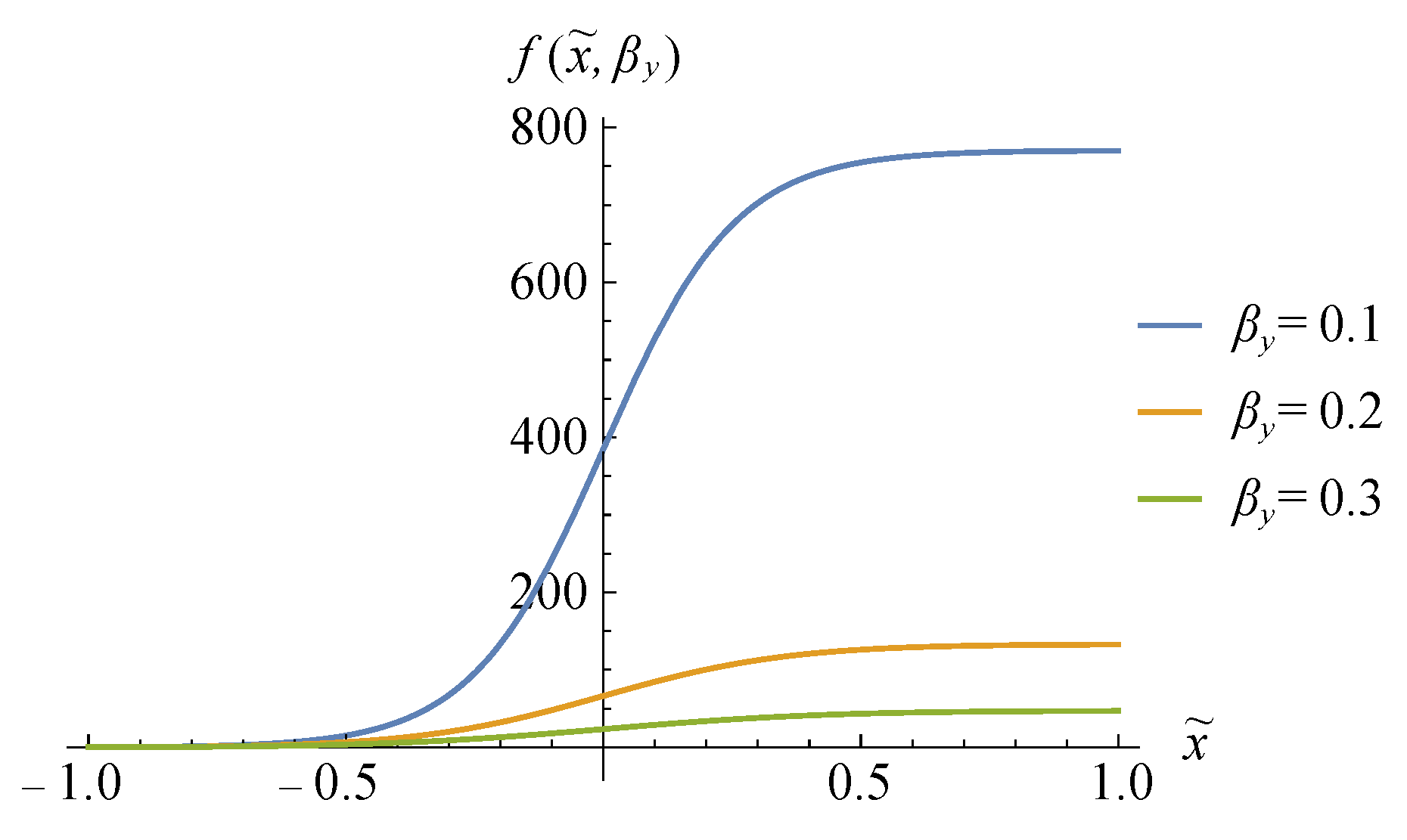
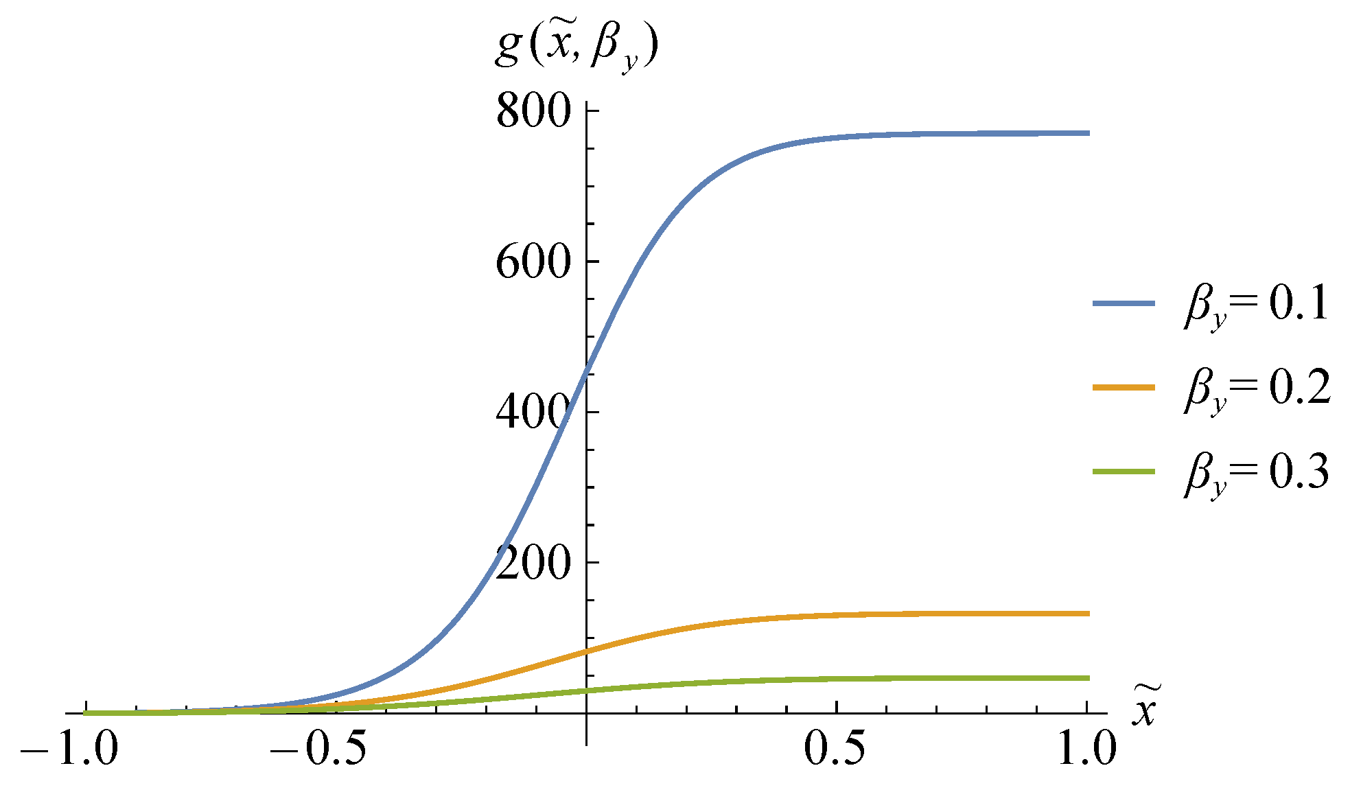
An analytical expression for $\tilde{\theta }\left(\tilde{x}\right)$ can be found from solving the integral in Equation (14), according to the results presented by Chen et al. [50], with some reworking. For the sake of conciseness, a compact form is here proposed:

$$\tilde{\theta }\left(\tilde{x}\right)=\frac{{\rho }^3{M}_f}{{Ea}_x^{2}l}f\left(\tilde{x},{\beta }_y\right)+{\mu }_Q{\rho }^{3}g\left(\tilde{x},{\beta }_y\right).$$

(37)

where ${\mu }_Q$ is defined, as analogously done for ${\mu }_F$ in Equation (24) referring to F, as ${\mu }_Q=\frac{Q}{El{a}_x}$. In Figure 9 and Figure 10, functions $f\left(\tilde{x},{\beta }_y\right)$ and $g\left(\tilde{x},{\beta }_y\right)$ are represented for some discrete values of ${\beta }_y$. As known in the literature [51], it is:

$$\sigma \left(x\right)=-E\kappa \left(x\right)y\left(x\right),$$

(38)

where $\sigma \left(x\right)$ represents the axial stress in the beam. The negative sign is due to the convention chosen; namely, a positive curvature means a counterclockwise rotation of the beam with the upper fibers compressed. Conventionally, a compression tension is considered negative.

Figure 9. Trend of function f in terms of $\tilde{x}$ and ${\beta }_y$.

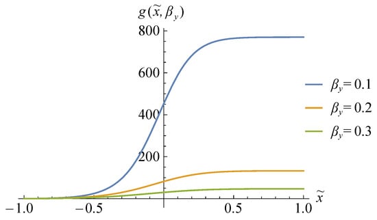
Figure 10. Trend of function g in terms of $\tilde{x}$ and ${\beta }_y$.

Equation (38) can be updated with the simplification made on $\kappa \left(x\right)$ and can be made dimensionless as follows:

$$\overline{\sigma }\left(\tilde{x}\right)=-\frac{E}{\rho }{\tilde{\theta }}^{\prime }\left(\tilde{x}\right)\tilde{y}\left(\tilde{x}\right).$$

(39)

In the first place, it is assumed that the most stressed section of the flexure is in $\tilde{x}=0$. When the maximum stress in the elastic domain is set in such a section, given by the yield stress ${\sigma }_{sn}$ of the material, the maximum moment that can be applied to the free end of the beam can be found for positive values of $y\left(x\right)$ as a function of $\rho$, ${\beta }_y$ and Q:

$$M_{f,max}=-a_{x}Q\pm \frac{2}{3}{a}_x^{2}l{\left(\frac{{\beta }_y}{\rho }\right)}^2{\sigma }_{sn},$$

(40)

where the positive sign in Equation (40) has to be chosen to have a counterclockwise rotation, whereas the negative sign has to be chosen to have a clockwise rotation.

Such equation results from a combination of Equations (5), (12), (14), (21) and (24) with Equation (39). It is demonstrated here below that the hypothesis of having the maximum stress in $\tilde{x}=0$. From this relation, Equation (40) is more valid when small values of ${\mu }_Q$ are considered in the module.

First of all, a development in the Taylor series of the stress $\overline{\sigma }\left(\tilde{x}\right)$ in Equation (39) up to the second order allows to look for stationary points. The maximum of $\overline{\sigma }\left(\tilde{x}\right)$ is obtained in:

$${\tilde{x}}_s=-{\displaystyle \frac{{\beta }_y}{2}}{\displaystyle \frac{1}{1+\frac{M_f}{l{a}_x^2{\mu }_{Q}E}}}.$$

(41)

The expression of the maximum moment $M_{f,max}$, assuming that a positive moment generates a counterclockwise rotation inducing a compressive tension on the fibers with positive $y\left(\tilde{x}\right)$, evaluated when $\overline{\sigma }\left({\tilde{x}}_s\right)=-{\sigma }_{sn}$, is:

$$M_{f,max}=-a_{x}Q\pm \left\{\frac{1}{3}{a}_x^{2}l{\left(\frac{{\beta }_y}{\rho }\right)}^2{\sigma }_{sn}+\sqrt{{\left[\frac{1}{3}{a}_x^{2}l{\left(\frac{{\beta }_y}{\rho }\right)}^2{\sigma }_{sn}\right]}^2-\frac{{\beta }_y}{4}{\left(a_{x}Q\right)}^2}\right\}.$$

(42)

The positive sign in Equation (42) has to be chosen to have a counterclockwise rotation, as already mentioned. The term in square brackets exists if $|{\mu }_Q|\le \frac{2}{3}\frac{{\beta }_y^{3/2}}{{\rho }^2}\frac{{\sigma }_{sn}}{E}$. The constraint on $|{\mu }_Q|$ imposes a limit to the possible values of Q. In particular, it is:

$$\begin{array}{cc}{\mu }_{Q,max}=\frac{2}{3}\frac{{\beta }_y^{3/2}}{{\rho }^2}\frac{{\sigma }_{sn}}{E};\hfill & {\mu }_{Q,min}=-\frac{2}{3}\frac{{\beta }_y^{3/2}}{{\rho }^2}\frac{{\sigma }_{sn}}{E}\end{array}.$$

(43)

A look at Equation (42) reveals that its expression tends to Equation (40) when the second term under the square root is negligible with respect to the first; namely, when:

$$|{\mu }_Q| <<\frac{2}{3}\frac{{\beta }_y^{3/2}}{{\rho }^2}\frac{{\sigma }_{sn}}{E}.$$

(44)

Therefore, the flexure is the more stressed at its geometric center; the smaller ${\mu }_Q$ is in modulus.

A final investigation can be directed towards the search for the expressions and trends of K and $\Delta M$, presented above. By calculating the integrals in Equation (16) and expressing them in terms of the nondimensional parameters $\rho$, ${\beta }_y$ and Q, it is:

$$\begin{array}{c}K={\displaystyle \frac{4{Ea}_x^{2}l}{3{\rho }^3}}{\displaystyle \frac{{\delta }_y{\left({\beta }_y{\gamma }_y\right)}^{\frac{5}{2}}}{6\sqrt{{\beta }_y{\gamma }_y}+8\sqrt{{\beta }_y^3{\gamma }_y}+4\sqrt{{\beta }_y^5{\gamma }_y}+3{\delta }_y^2\left[\pi +2{csc}^{-1}\left({\delta }_y\right)\right]}}\\ \Delta M=-a_{x}Q\end{array}.$$

(45)

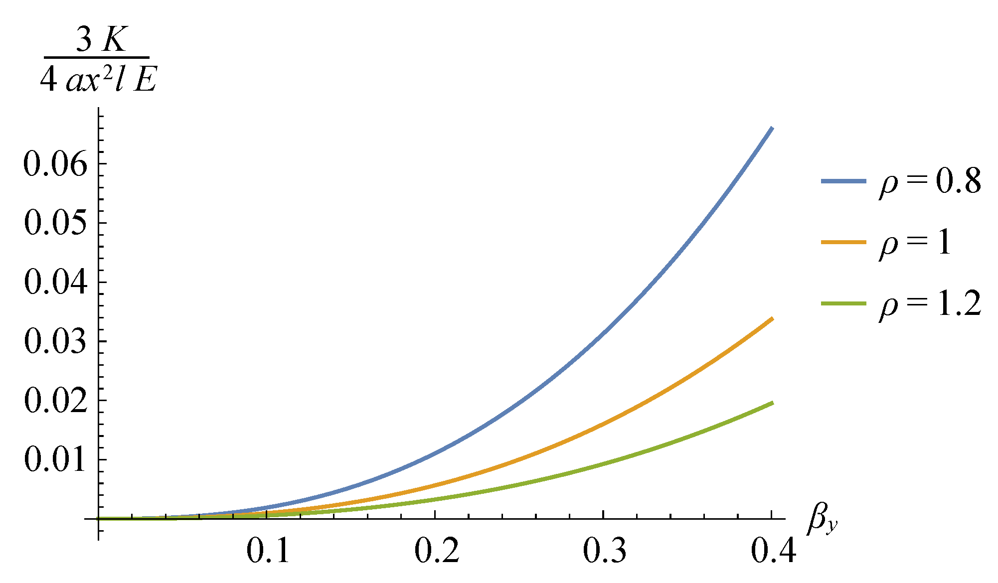
It can be observed from Equation (45) that, except for the Young’s Modulus, coefficient K depends only on the beam geometry, whereas the dependence on the loads can be found only in $\Delta M$. The stiffness coefficient K mainly depends on the beam geometry. Its trend is shown in Figure 11 when ${\beta }_y$ and $\rho$ vary. In addition, it can be observed that in order to have a low value of stiffness K, which corresponds to a large rotation without excessive tension of the material, high values of $\rho$ are preferred and, conversely, low values of ${\beta }_y$.

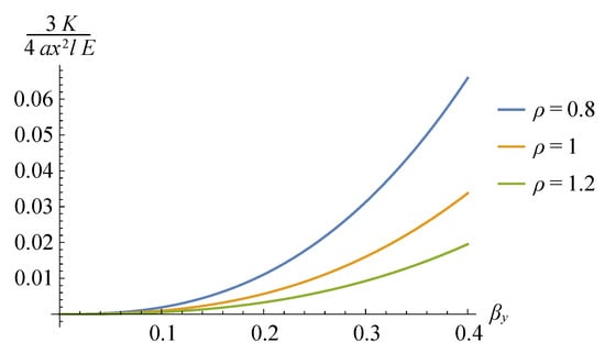
Figure 11. Trend of function K in terms of ${\beta }_y$ and $\rho$.

Regarding parameter $\Delta M$, it is easy to verify that when it is null, the classical linear relation between $M_f$ and ${\theta }_f$ is obtained, namely: $M_f=K{\theta }_f$. Moreover, by looking at the second expression in Equation (45), the right side of the equation represents the first addendum in Equation (42). With reference to the results presented in Equations (42) and (44) and remembering the definition of ${\mu }_Q$, the following expressions of $M_f$ and Q can be imposed introducing the two coefficients ${\alpha }_Q$ and ${\alpha }_M$:

$$\begin{array}{cc}Q={\alpha }_{Q}El{a}_x{\mu }_{Q,max}& \\ M_f={\alpha }_M{M}_{f,max}\end{array}$$

(46)

where ${\alpha }_M\in [0;1]$ and ${\alpha }_Q\in [-1;1]$. The smaller ${\alpha }_Q$ is in modulus, the more the maximum stress is in the middle section of the flexure joint. On the other hand, the smaller ${\alpha }_M$ is, the further away from the yield condition.

An analytical study of ${\theta }_f$ allows us to evaluate its maximum value. In particular, it occurs when ${\alpha }_M=1$ and ${\alpha }_Q=0$, namely for a pure bending load:

$${\theta }_{f,max}=\pm \frac{2}{3}{a}_x^{2}l{\left(\frac{{\beta }_y}{\rho }\right)}^2\frac{{\sigma }_{sn}}{K}.$$

(47)

5. Domain of Application of the Linear Model

All the models presented so far are based on the assumption that the flexure hinge behaves like a beam. Therefore, it must be ensured that this assumption is admissible.

It is certainly known that a three-dimensional solid behaves like a beam when one of its dimensions is about ten times larger than the other two. The flexure hinge under study has two constant dimensions (length and depth), whereas the height is variable.

Since the flexure hinge has to be compliant with rotations about the z-axis, its depth has to result from a compromise between transversal compliance and bending stiffness.

With reference to Figure 5 and Equation (18), the length and the mean height of the flexure hinge from $-x$ to x are equal to:

$$\begin{array}{cc}L\left(x\right)=2x& \\ \overline{H}\left(x\right)=\frac{1}{2x}{\int }_{-x}^{x}2y\left(\tau \right)d\tau .\end{array}$$

(48)

From the previous two relations, the ratio between the length and the mean height is given by:

$$r\left(x\right)=\frac{4x^2}{{\int }_{-x}^{x}2y\left(\tau \right)d\tau }$$

(49)

Because the formula for $y\left(\tilde{x}\right)$ has a complex nonlinear expression, a Taylor series expansion is used for expression in Equation (49), up to a fourth-order truncation error, in order to be precise enough but at the same time have a simple resulting expression. It follows:

$$r_T\left(x\right)=\frac{\rho }{{\beta }_y}\frac{x}{a_x}-\frac{\rho }{6{\beta }_y^2}{\left(\frac{x}{a_x}\right)}^3$$

(50)

Imposing the derivative of Equation (50) equal to zero and solving the resulting equation, the position along the axis of the flexure hinge where the ratio $r_T\left(x\right)$ is maximum can be found. In particular, it is:

$$\begin{array}{cc}{x}_r=\pm a_x\sqrt{2{\beta }_y}& \\ r_{T,x_r}=\frac{2\sqrt{2}}{3}\frac{\rho }{\sqrt{{\beta }_y}}\end{array}.$$

(51)

Assuming the condition $r_{T,x_r}\ge 10$, the following condition must apply:

$$\rho \ge 15\sqrt{\frac{{\beta }_y}{2}}$$

(52)

From Equations (39) and (46), it is possible to evaluate the stress in $x_r$. Assuming ${\alpha }_M=1$ and ${\alpha }_Q=0$, it follows:

$$|{\sigma }_{{\tilde{x}}_r}|=\frac{{\beta }_y^2}{2+{\beta }_y^2-2\sqrt{1-2{\beta }_y}(1+{\beta }_y)}{\sigma }_{sn}$$

(53)

where ${\tilde{x}}_r=\frac{x}{a_x}$.

A limit for ${\beta }_y$ is obtained from the previous relation, in particular ${\beta }_y\in \left]0;\frac{1}{2}\right]$. Evaluating the mean absolute value of the stress in Equation (53) in the range mentioned for ${\beta }_y$, a value of about $0.2{\sigma }_{sn}$ is obtained.

It follows that the area of the flexure hinge with length equal to $2a_x\sqrt{2{\beta }_y}$, namely $2|x_r|$, is the most stressed. Therefore, it is correct to consider it as the reference hinge length to evaluate the depth to be assigned to the joint, not the whole length of the flexure hinge.

Assuming $\frac{2\left|x_r\right|}{l}=r_{T,x_r}$ and that condition Equation (52) is verified, then it follows:

$$l\le \frac{\sqrt{2}}{5}\sqrt{{\beta }_y}{a}_x$$

(54)

6. Comparison of Analytical and Numerical Solutions

In this section, a comparison is presented between the solutions obtained applying the linear analytical model, solving numerically the second differential equation in Equation (3) and by means of Finite Element (FE) simulations using the software ANSYS, estimating the error due to the approximations made. Each simplifying assumption, namely the negligibility of the axial deformation, the effect of linearization due to small rotations, and the negligibility of the axial load F, has been considered. In the absence of experimental data, the values obtained from FE simulations are taken as a reference to evaluate the errors made from the nonlinear model through the series of approximations. FE analyses were performed on a three-dimensional elliptical flexure with depth derived from Equation (54) when the equal sign is taken. They are provided in more detail in a previous work of the same authors [42]. Still, some information can be recalled here: the model of the flexure hinge was divided into three parts in order to refine the mesh in the thinnest central area. The whole number of nodes was about $5·{10}^5$, and a quadratic element with a “Hex Dominant” mesh method was used in the central area of the flexure hinge. In all the analyses, an elliptical flexure hinge made of steel with $a_x=1$ has been taken into account ($E=210$ GPa and ${\sigma }_{sn}=600$ MPa). Finally, the force F acting at the free end of the beam can be defined by using the expression in Equation (25):

$$F={\alpha }_F\frac{2}{3}El{a}_x{\left(\frac{{\beta }_y}{\rho }\right)}^3$$

(55)

where ${\alpha }_F\in [-1;1]$. The smaller ${\alpha }_F$ is, in modulus, the more the condition in Equation (25) is verified. That is, the analytical solution well describes the behavior of the flexure joint.

Some cases of interest are presented in the following varying the dimensionless parameters $\rho$, ${\beta }_y$, ${\alpha }_F$, ${\alpha }_Q$ and ${\alpha }_M$ in their range of existence: ${\beta }_y\in \left]0;\frac{1}{2}\right]$, $\left({\alpha }_F,{\alpha }_Q\right)\in [-1;1]$ and ${\alpha }_M\in [0;1]$. The proposed studies are not intended to be exhaustive but only to give an idea of the behavior of an elliptical flexure joint as the most significant parameters change.

6.1. Case I

In this first case study, a fixed value is assigned to $\rho$, ${\beta }_y$, ${\alpha }_Q$, and ${\alpha }_M$, while parameter ${\alpha }_F$ is left free in order to analyze its effect on the rotation ${\theta }_f$ of the free end of the beam. The flexure hinge is considered in the most stressed condition, namely when ${\alpha }_Q=0$ and ${\alpha }_M=1$, whereas the values of $\rho$ and ${\beta }_y$ are chosen respectively equal to 15 and $0.1$. The resulting values of ${\theta }_f$ are collected in Table 1, where the superscript + indicates the choice of the positive sign in Equation (42). Entirely similar results but mirrored in the signs, in agreement with the absence of the transversal force Q, are obtained for negative rotations, in the following indicated by the superscript −.

Table 1. CASE I—Comparison between analytical and numerical models with $\rho$, ${\beta }_y$, ${\alpha }_Q$ and ${\alpha }_M$ fixed while ${\alpha }_F$ varies.

${\mathit{\alpha }}_{\mathit{F}}$	${\mathit{\theta }}_{\mathit{f},\mathit{A}}^{+}\left[{}^{\circ }\right]$	${\mathit{\theta }}_{\mathit{f},\mathit{n}}^{+}\left[{}^{\circ }\right]$	${\mathit{\theta }}_{\mathit{f},\mathit{n}-\mathit{\epsilon }}^{+}\left[{}^{\circ }\right]$	${\mathit{\theta }}_{\mathit{f},\mathit{n}-\mathit{T}}^{+}\left[{}^{\circ }\right]$	${\mathit{\theta }}_{\mathit{f},\mathit{n}-\mathit{a}\left(\tilde{\mathit{x}}\right)}^{+}\left[{}^{\circ }\right]$	${\mathit{\theta }}_{\mathit{f},\mathbf{FEM}}^{+}\left[{}^{\circ }\right]$
$1.00$	$12.605$	$8.740$	$8.740$	$8.731$	$12.605$	$8.744$
$0.50$	$12.605$	$10.316$	$10.316$	$10.308$	$12.605$	$10.322$
$0.10$	$12.605$	$12.069$	$12.069$	$12.065$	$12.605$	$12.075$
$0.05$	$12.605$	$12.331$	$12.331$	$12.329$	$12.605$	$12.337$
$0.01$	$12.605$	$12.549$	$12.549$	$12.549$	$12.605$	$12.555$
$-0.01$	$12.605$	$12.661$	$12.661$	$12.662$	$12.605$	$12.668$
$-0.05$	$12.605$	$12.892$	$12.892$	$12.894$	$12.605$	$12.898$
$-0.10$	$12.605$	$13.192$	$13.192$	$13.197$	$12.605$	$13.199$
$-0.50$	$12.605$	$16.209$	$16.209$	$16.264$	$12.605$	$16.218$
$-1.00$	$12.605$	$22.582$	$22.582$	$23.010$	$12.605$	$22.593$
${\mathbf{\alpha }}_{\mathbf{F}}$	${\mathbf{\Delta }}_{\mathit{n}\mathit{,}\mathit{A}}\mathbf{\%}$	${\mathit{\delta }}_{\mathit{\epsilon }}\mathbf{\%}$	${\mathit{\delta }}_{\mathit{T}}\mathbf{\%}$	${\mathbf{\delta }}_{\mathit{a}\left(\tilde{\mathit{x}}\right)}\mathbf{\%}$	${\mathbf{\Delta }}_{\mathit{FEM}\mathbf{,}\mathit{A}}\mathrm{\%}$
$1.00$	$44.224$	$1.76\times {10}^{-7}$	$0.103$	$44.223$	$44.16$
$0.50$	$22.183$	$1.27\times {10}^{-7}$	$0.086$	$22.183$	$22.12$
$0.10$	$4.446$	$3.42\times {10}^{-8}$	$0.028$	$4.445$	$4.39$
$0.05$	$2.223$	$1.78\times {10}^{-8}$	$0.015$	$2.223$	$2.17$
$0.01$	$0.445$	$3.66\times {10}^{-9}$	$0.003$	$0.445$	$0.40$
$-0.01$	$0.444$	$3.72\times {10}^{-9}$	$0.003$	$0.445$	$0.50$
$-0.05$	$2.223$	$1.92\times {10}^{-8}$	$0.017$	$2.224$	$2.27$
$-0.10$	$4.447$	$3.98\times {10}^{-8}$	$0.036$	$4.448$	$4.50$
$-0.50$	$22.234$	$2.72\times {10}^{-7}$	$0.342$	$22.234$	$22.28$
$-1.00$	$44.180$	$8.32\times {10}^{-7}$	$1.895$	$44.180$	$44.21$

From Equation (47), the constant value of ${\theta }_f$ resulting from the analytical solution was predictable, but the numerical solution presented in Table 1 reveals that ${\theta }_F$ depends on ${\alpha }_F$.

In Table 1 the subscripts used in defining ${\theta }_f$ have the following meaning: ${\theta }_{f,A}$ refers to the analytical value obtained with Equation (47), ${\theta }_{f,n}$, ${\theta }_{f,n-\epsilon }$, ${\theta }_{f,n-T}$ and ${\theta }_{f,n-a\left(\tilde{x}\right)}$ are respectively the numerical solutions of the second equation in Equation (3) for the complete model, a simplified model where only the axial deformation $\epsilon$ is neglected, yet a simplified model where the trigonometric functions are linearized and eventually another simplified model where the effect of the axial load F is neglected. As a reference, ${\theta }_{f,FEM}$ is the numerical value obtained by means of FE simulations.

In addition, symbols ${\Delta }_{(.)}\%$ and ${\delta }_{(.)}\%$ in the tables are percentage errors defined as:

$$\begin{array}{cc}{\Delta }_{n,A}\%=100\left|{\displaystyle \frac{{\theta }_{f,n}-{\theta }_{f,A}}{{\theta }_{f,n}}}\right|& \\ {\Delta }_{FEM,A}\%=100\left|\frac{{\theta }_{f,FEM}-{\theta }_{f,A}}{{\theta }_{f,FEM}}\right|& \\ {\delta }_{\epsilon }\%=100\left|{\displaystyle \frac{{\theta }_{f,n}-{\theta }_{f,n-\epsilon }}{{\theta }_{f,n}}}\right|& \\ {\delta }_T\%=100\left|{\displaystyle \frac{{\theta }_{f,n}-{\theta }_{f,n-T}}{{\theta }_{f,n}}}\right|& \\ {\delta }_{a\left(\tilde{x}\right)}\%=100\left|{\displaystyle \frac{{\theta }_{f,n}-{\theta }_{f,n-a\left(\tilde{x}\right)}}{{\theta }_{f,n}}}\right|.\end{array}$$

(56)

From Table 1 and Figure 12 and Figure 13, it can be observed that the approximation of neglecting $\epsilon$ and the linearization of the trigonometric functions are practically verified in the whole range of ${\alpha }_F$. On the contrary, the negligibility of the effect of the axial load F is increasingly allowed when ${\alpha }_F$ is small in absolute value. Furthermore, the values obtained with the FE analyses are in agreement with those obtained numerically. It can also be noted that the error decreases as ${\alpha }_F$ decreases, which demonstrates the impact of the axial force on the model accuracy.

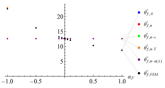
Figure 12. CASE I—Trend of ${\theta }_f$ evaluated analytically and numerically.

Figure 13. CASE I—Trend of the various percentage errors.

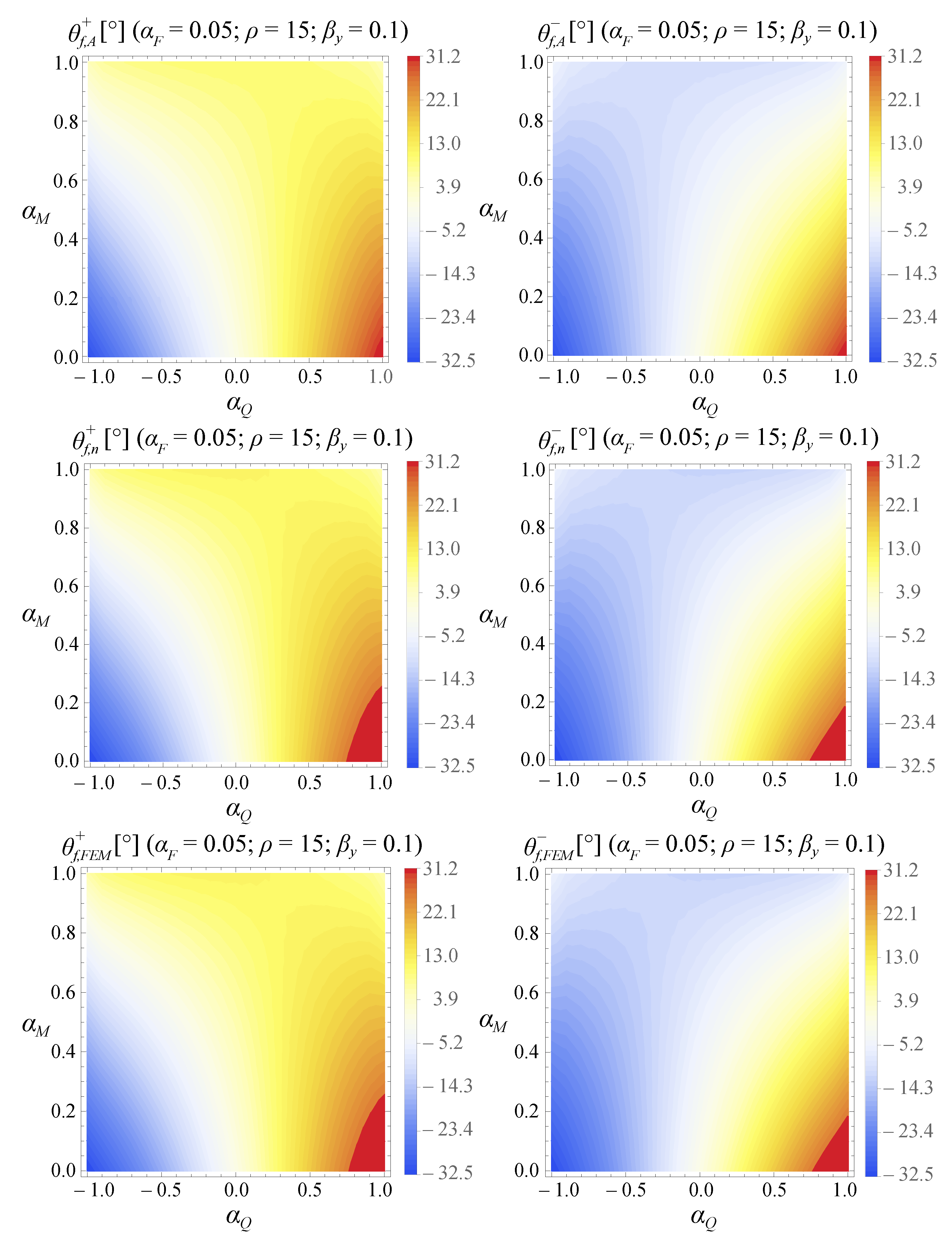
6.2. Case II

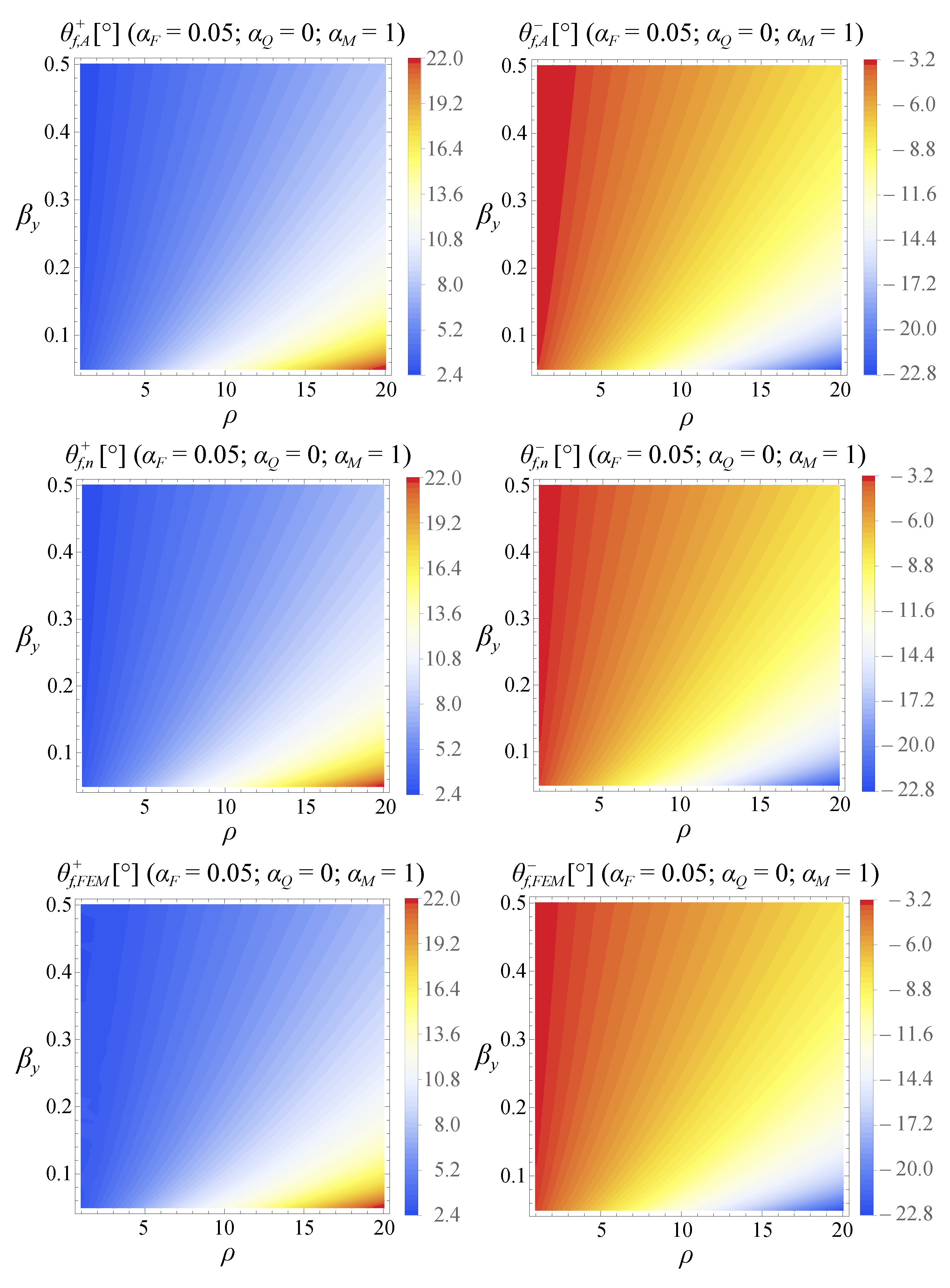
In the second case study, the effects of $\rho$ and ${\beta }_y$ on the rotation ${\theta }_F$ are analyzed when the other parameters are fixed. In particular, their values are chosen as follows: ${\alpha }_F=0.05$, ${\alpha }_Q=0$ and ${\alpha }_M=1$.

Results are shown in Table Table 2 and in the sensitivity maps of Figure 14. In the latter, the values of ${\theta }_F$ evaluated analytically, numerically, and by means of FE simulations are shown. Even in this case, the absence of the tangential force Q provides mirrored values for negative rotations.

Table 2. CASE II—Comparison between analytical and numerical models with ${\alpha }_F$, ${\alpha }_Q$ and ${\alpha }_M$ fixed while $\rho$ and ${\beta }_y$ vary.

$\mathit{\rho }$	${\mathit{\beta }}_{\mathit{y}}$	${\mathit{\theta }}_{\mathit{f},\mathit{A}}^{+}\left[{}^{\circ }\right]$	${\mathit{\theta }}_{\mathit{f},\mathit{n}}^{+}\left[{}^{\circ }\right]$	${\mathit{\theta }}_{\mathit{f},\mathit{n}-\mathit{\epsilon }}^{+}\left[{}^{\circ }\right]$	${\mathit{\theta }}_{\mathit{f},\mathit{n}-\mathit{T}}^{+}\left[{}^{\circ }\right]$	${\mathit{\theta }}_{\mathit{f},\mathit{n}-\mathit{a}\left(\tilde{\mathit{x}}\right)}^{+}\left[{}^{\circ }\right]$	${\mathit{\theta }}_{\mathit{f},\mathbf{FEM}}^{+}\left[{}^{\circ }\right]$
5	$0.050$	$6.021$	$5.922$	$5.922$	$5.922$	$6.021$	$5.929$
5	$0.175$	$3.113$	$3.029$	$3.029$	$3.029$	$3.113$	$3.074$
5	$0.300$	$2.300$	$2.225$	$2.225$	$2.225$	$2.300$	$2.301$
10	$0.050$	$12.042$	$11.846$	$11.846$	$11.845$	$12.042$	$11.849$
10	$0.175$	$6.226$	$6.057$	$6.057$	$6.057$	$6.226$	$6.077$
10	$0.300$	$4.600$	$4.449$	$4.449$	$4.449$	$4.600$	$4.483$
15	$0.050$	$18.063$	$17.771$	$17.771$	$17.767$	$18.063$	$17.773$
15	$0.175$	$9.339$	$9.087$	$9.087$	$9.086$	$9.339$	$9.099$
15	$0.300$	$6.900$	$6.674$	$6.674$	$6.674$	$6.900$	$6.696$
$\mathit{\rho }$	${\mathit{\beta }}_{\mathit{y}}$	${\mathbf{\Delta }}_{\mathit{n}\mathbf{,}\mathit{A}}\mathbf{\%}$	${\mathit{\delta }}_{\mathit{\epsilon }}\mathbf{\%}$	${\mathit{\delta }}_{\mathit{T}}\mathbf{\%}$	${\mathbf{\delta }}_{\mathit{a}\left(\tilde{\mathit{x}}\right)}\mathbf{\%}$	${\mathbf{\Delta }}_{\mathit{FEM}\mathbf{,}\mathit{A}}\mathbf{\%}$
5	$0.050$	$1.664$	$1.28\times {10}^{-7}$	$0.003$	$1.664$	$1.556$
5	$0.175$	$2.792$	$1.35\times {10}^{-6}$	$0.001$	$2.791$	$1.279$
5	$0.300$	$3.391$	$3.48\times {10}^{-6}$	$0.001$	$3.390$	$0.043$
10	$0.050$	$1.656$	$1.60\times {10}^{-8}$	$0.011$	$1.655$	$1.627$
10	$0.175$	$2.789$	$1.69\times {10}^{-7}$	$0.004$	$2.788$	$2.453$
10	$0.300$	$3.388$	$4.34\times {10}^{-7}$	$0.003$	$3.388$	$2.614$
15	$0.050$	$1.642$	$4.70\times {10}^{-9}$	$0.024$	$1.642$	$1.633$
15	$0.175$	$2.783$	$5.00\times {10}^{-8}$	$0.010$	$2.783$	$2.639$
15	$0.300$	$3.385$	$1.29\times {10}^{-7}$	$0.006$	$3.385$	$3.051$

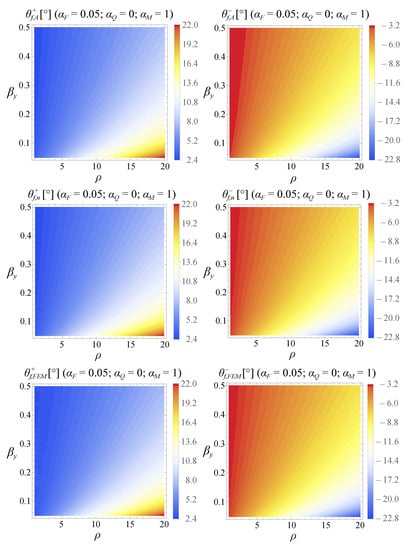
Figure 14. CASE II—Trend of ${\theta }_F$ evaluated analytically, numerically and by FE simulations varying $\rho$ and ${\beta }_y$.

From Table Table 2 and Figure 15, it can be noted that the error decreases as ${\beta }_y$ decreases while remaining constant as $\rho$ is varying. Furthermore, it can be observed that the angular displacements increase when ${\beta }_y$ decreases and when $\rho$ increases as well.

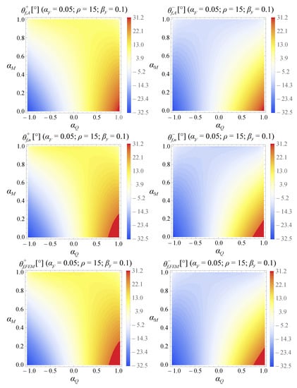
Figure 15. CASE III—Trend of ${\theta }_F$ evaluated analytically, numerically and by FE simulations, varying ${\alpha }_Q$ and ${\alpha }_M$.

6.3. Case III

In this last case study, the effects of ${\alpha }_Q$ and ${\alpha }_M$ on the rotation ${\theta }_F$ are analyzed when the other parameters are fixed. In the analyses, the following parameter values are chosen: ${\alpha }_F=0.05$, $\rho =15$ and ${\beta }_y=0.1$.

Results are shown in Table 3 and Table 4 and in the sensitivity maps of Figure 15. From the tables and the figure, it can be noted that the error decreases as ${\alpha }_Q$, in absolute value, decreases and ${\alpha }_M$ increases. Furthermore, it can be observed that the angular displacements increase when ${\alpha }_M$ decreases and when ${\alpha }_Q$ approaches 1 in absolute value.

Table 3. CASE III—Comparison between analytical and numerical models for positive rotations with ${\alpha }_F$, $\rho$ and ${\beta }_y$ fixed while ${\alpha }_Q$ and ${\alpha }_M$ vary.

${\mathit{\alpha }}_{\mathit{Q}}$	${\mathit{\alpha }}_{\mathit{M}}$	${\mathit{\theta }}_{\mathit{f},\mathit{A}}^{+}\left[{}^{\circ }\right]$	${\mathit{\theta }}_{\mathit{f},\mathit{n}}^{+}\left[{}^{\circ }\right]$	${\mathit{\theta }}_{\mathit{f},\mathit{n}-\mathit{\epsilon }}^{+}\left[{}^{\circ }\right]$	${\mathit{\theta }}_{\mathit{f},\mathit{n}-\mathit{T}}^{+}\left[{}^{\circ }\right]$	${\mathit{\theta }}_{\mathit{f},\mathit{n}-\mathit{a}\left(\tilde{\mathit{x}}\right)}^{+}\left[{}^{\circ }\right]$	${\mathit{\theta }}_{\mathit{f},\mathit{FEM}}^{+}\left[{}^{\circ }\right]$
$-1.0$	$0.1$	$-35.244$	$-30.001$	$-30.001$	$-34.446$	$-30.516$	$-30.013$
$-0.5$	$0.1$	$-16.761$	$-15.758$	$-15.758$	$-16.381$	$-16.093$	$-15.765$
$-0.1$	$0.1$	$-2.330$	$-2.274$	$-2.274$	$-2.276$	$-2.327$	$-2.275$
$0.1$	$0.1$	$4.845$	$4.725$	$4.725$	$4.736$	$4.833$	$4.727$
$0.5$	$0.1$	$19.113$	$17.887$	$17.887$	$18.682$	$18.260$	$17.895$
$1.0$	$0.1$	$36.505$	$30.962$	$30.962$	$35.679$	$31.488$	$30.974$
$-1.0$	$0.5$	$-16.779$	$-15.153$	$-15.153$	$-16.385$	$-15.464$	$-15.157$
$-0.5$	$0.5$	$-4.085$	$-3.935$	$-3.935$	$-3.982$	$-4.034$	$-3.935$
$-0.1$	$0.5$	$4.294$	$4.211$	$4.211$	$4.202$	$4.302$	$4.213$
$0.1$	$0.5$	$8.280$	$8.065$	$8.065$	$8.096$	$8.246$	$8.069$
$0.5$	$0.5$	$15.846$	$14.924$	$14.924$	$15.485$	$15.243$	$14.930$
$1.0$	$0,5$	$23.082$	$20.401$	$20.401$	$22.550$	$20.792$	$20.408$
$-1.0$	$0.9$	$1.686$	$1.690$	$1.690$	$1.676$	$1.700$	$1.693$
$-0.5$	$0.9$	$8.592$	$8.577$	$8.577$	$8.417$	$8.762$	$8.583$
$-0.1$	$0.9$	$10.918$	$10.737$	$10.737$	$10.681$	$10.975$	$10.743$
$0.1$	$0.9$	$11.715$	$11.394$	$11.394$	$11.456$	$11.647$	$11.400$
$0.5$	$0.9$	$12.578$	$11.924$	$11.924$	$12.289$	$12.186$	$11.929$
$1.0$	$0.9$	$9.658$	$8.947$	$8.947$	$9.420$	$9.153$	$8.948$
${\mathit{\alpha }}_{\mathit{Q}}$	${\mathit{\alpha }}_{\mathit{M}}$	${\mathbf{\Delta }}_{\mathit{n}\mathbf{,}\mathit{A}}\mathbf{\%}$	${\mathit{\delta }}_{\mathit{\epsilon }}\mathbf{\%}$	${\mathit{\delta }}_{\mathit{T}}\mathbf{\%}$	${\mathit{\delta }}_{\mathit{a}\left(\tilde{\mathit{x}}\right)}\mathbf{\%}$	${\mathbf{\Delta }}_{\mathit{FEM}\mathbf{,}\mathit{A}}\mathbf{\%}$
$-1.0$	$0.1$	$17.476$	$5.32\times {10}^{-7}$	$14.816$	$1.717$	$17.429$
$-0.5$	$0.1$	$6.365$	$2.22\times {10}^{-7}$	$3.954$	$2.126$	$6.318$
$-0.1$	$0.1$	$2.463$	$9.13\times {10}^{-8}$	$0.088$	$2.331$	$2.418$
$0.1$	$0.1$	$2.540$	$6.71\times {10}^{-8}$	$0.233$	$2.286$	$2.496$
$0.5$	$0.1$	$6.854$	$2.21\times {10}^{-7}$	$4.445$	$2.085$	$6.806$
$1.0$	$0.1$	$17.903$	$5.30\times {10}^{-7}$	$15.235$	$1.699$	$17.857$
$-1.0$	$0.5$	$10.731$	$5.99\times {10}^{-7}$	$8.130$	$2.052$	$10.701$
$-0.5$	$0.5$	$3.812$	$3.21\times {10}^{-7}$	$1.194$	$2.516$	$3.812$
$-0.1$	$0.5$	$1.971$	$1.03\times {10}^{-8}$	$0.214$	$2.161$	$1.923$
$0.1$	$0.5$	$2.666$	$5.93\times {10}^{-8}$	$0.384$	$2.244$	$2.615$
$0.5$	$0.5$	$6.178$	$2.23\times {10}^{-7}$	$3.759$	$2.137$	$6.135$
$1.0$	$0.5$	$13.142$	$5.67\times {10}^{-7}$	$10.534$	$1.917$	$13.103$
$-1.0$	$0.9$	$0.237$	$6.55\times {10}^{-7}$	$0.828$	$0.592$	$0.413$
$-0.5$	$0.9$	$0.175$	$4.12\times {10}^{-8}$	$1.865$	$2.157$	$0.105$
$-0.1$	$0.9$	$1.686$	$2.21\times {10}^{-8}$	$0.522$	$2.217$	$1.629$
$0.1$	$0.9$	$2.817$	$4.73\times {10}^{-8}$	$0.544$	$2.220$	$2.763$
$0.5$	$0.9$	$5.485$	$2.28\times {10}^{-7}$	$3.061$	$2.197$	$5.441$
$1.0$	$0.9$	$7.947$	$6.82\times {10}^{-7}$	$5.287$	$2.302$	$7.935$

Table 4. CASE III—Comparison between analytical and numerical models for negative rotations with ${\alpha }_F$, $\rho$ and ${\beta }_y$ fixed varying ${\alpha }_Q$ and ${\alpha }_M$.

${\mathit{\alpha }}_{\mathit{Q}}$	${\mathit{\alpha }}_{\mathit{M}}$	${\mathit{\theta }}_{\mathit{f},\mathit{A}}^{-}\left[{}^{\circ }\right]$	${\mathit{\theta }}_{\mathit{f},\mathit{n}}^{-}\left[{}^{\circ }\right]$	${\mathit{\theta }}_{\mathit{f},\mathit{n}-\mathit{\epsilon }}^{-}\left[{}^{\circ }\right]$	${\mathit{\theta }}_{\mathit{f},\mathit{n}-\mathit{T}}^{-}\left[{}^{\circ }\right]$	${\mathit{\theta }}_{\mathit{f},\mathit{n}-\mathit{a}\left(\tilde{\mathit{x}}\right)}^{-}\left[{}^{\circ }\right]$	${\mathit{\theta }}_{\mathit{f},\mathit{FEM}}^{-}\left[{}^{\circ }\right]$
$-1.0$	$0.1$	$-36.505$	$-30.962$	$-30.962$	$-35.679$	$-31.488$	$-30.974$
$-0.5$	$0.1$	$-19.113$	$-17.887$	$-17.887$	$-18.682$	$-18.26$	$-17.895$
$-0.1$	$0.1$	$-4.845$	$-4.725$	$-4.725$	$-4.736$	$-4.833$	$-4.727$
$0.1$	$0.1$	$2.330$	$2.274$	$2.274$	$2.276$	$2.327$	$2.275$
$0.5$	$0.1$	$16.761$	$15.758$	$15.758$	$16.381$	$16.093$	$15.765$
$1.0$	$0.1$	$35.244$	$30.001$	$30.001$	$34.446$	$30.516$	$30.012$
$-1.0$	$0.5$	$-23.082$	$-20.401$	$-20.401$	$-22.55$	$-20.792$	$-20.408$
$-0.5$	$0.5$	$-15.846$	$-14.924$	$-14.924$	$-15.485$	$-15.243$	$-14.93$
$-0.1$	$0.5$	$-8.280$	$-8.065$	$-8.065$	$-8.096$	$-8.246$	$-8.069$
$0.1$	$0.5$	$-4.294$	$-4.211$	$-4.211$	$-4.202$	$-4.302$	$-4.213$
$0.5$	$0.5$	$4.085$	$3.935$	$3.935$	$3.982$	$4.034$	$3.935$
$1.0$	$0.5$	$16.779$	$15.153$	$15.153$	$16.385$	$15.464$	$15.157$
$-1.0$	$0.9$	$-9.658$	$-8.947$	$-8.947$	$-9.420$	$-9.153$	$-8.948$
$-0.5$	$0.9$	$-12.578$	$-11.924$	$-11.924$	$-12.289$	$-12.186$	$-11.929$
$-0.1$	$0.9$	$-11.715$	$-11.394$	$-11.394$	$-11.456$	$-11.647$	$-11.400$
$0.1$	$0.9$	$-10.918$	$-10.737$	$-10.737$	$-10.681$	$-10.975$	$-10.743$
$0.5$	$0.9$	$-8.592$	$-8.577$	$-8.577$	$-8.417$	$-8.762$	$-8.583$
$1.0$	$0.9$	$-1.686$	$-1.690$	$-1.690$	$-1.676$	$-1.700$	$-1.693$
${\mathit{\alpha }}_{\mathit{Q}}$	${\mathit{\alpha }}_{\mathit{M}}$	${\mathbf{\Delta }}_{\mathit{n}\mathbf{,}\mathit{A}}\mathbf{\%}$	${\mathit{\delta }}_{\mathit{\epsilon }}\mathbf{\%}$	${\mathit{\delta }}_{\mathit{T}}\mathbf{\%}$	${\mathit{\delta }}_{\mathit{a}\left(\tilde{\mathit{x}}\right)}\mathbf{\%}$	${\mathbf{\Delta }}_{\mathit{FEM}\mathbf{,}\mathit{A}}\mathbf{\%}$
$-1.0$	$0.1$	$17.903$	$2.65\times {10}^{-7}$	$15.235$	$1.699$	$17.857$
$-0.5$	$0.1$	$6.854$	$1.11\times {10}^{-7}$	$4.445$	$2.085$	$6.806$
$-0.1$	$0.1$	$2.540$	$3.35\times {10}^{-8}$	$0.233$	$2.286$	$2.496$
$0.1$	$0.1$	$2.463$	$4.56\times {10}^{-8}$	$0.088$	$2.331$	$2.418$
$0.5$	$0.1$	$6.365$	$1.11\times {10}^{-7}$	$3.954$	$2.126$	$6.318$
$1.0$	$0.1$	$17.476$	$2.66\times {10}^{-7}$	$14.816$	$1.717$	$17.433$
$-1.0$	$0.5$	$13.142$	$2.84\times {10}^{-7}$	$10.534$	$1.917$	$13.103$
$-0.5$	$0.5$	$6.178$	$1.11\times {10}^{-7}$	$3.759$	$2.137$	$6.135$
$-0.1$	$0.5$	$2.666$	$2.96\times {10}^{-8}$	$0.384$	$2.244$	$2.615$
$0.1$	$0.5$	$1.971$	$5.18\times {10}^{-9}$	$0.214$	$2.161$	$1.923$
$0.5$	$0.5$	$3.812$	$1.61\times {10}^{-7}$	$1.194$	$2.516$	$3.812$
$1.0$	$0.5$	$10.731$	$3.00\times {10}^{-7}$	$8.130$	$2.052$	$10.701$
$-1.0$	$0.9$	$7.947$	$3.41\times {10}^{-7}$	$5.287$	$2.302$	$7.935$
$-0.5$	$0.9$	$5.485$	$1.14\times {10}^{-7}$	$3.061$	$2.197$	$5.441$
$-0.1$	$0.9$	$2.817$	$2.86\times {10}^{-8}$	$0.544$	$2.220$	$2.763$
$0.1$	$0.9$	$1.686$	$1.10\times {10}^{-8}$	$0.522$	$2.217$	$1.629$
$0.5$	$0.9$	$0.175$	$2.06\times {10}^{-8}$	$1.865$	$2.157$	$0.105$
$1.0$	$0.9$	$0.237$	$3.28\times {10}^{-7}$	$0.828$	$0.592$	$0.413$

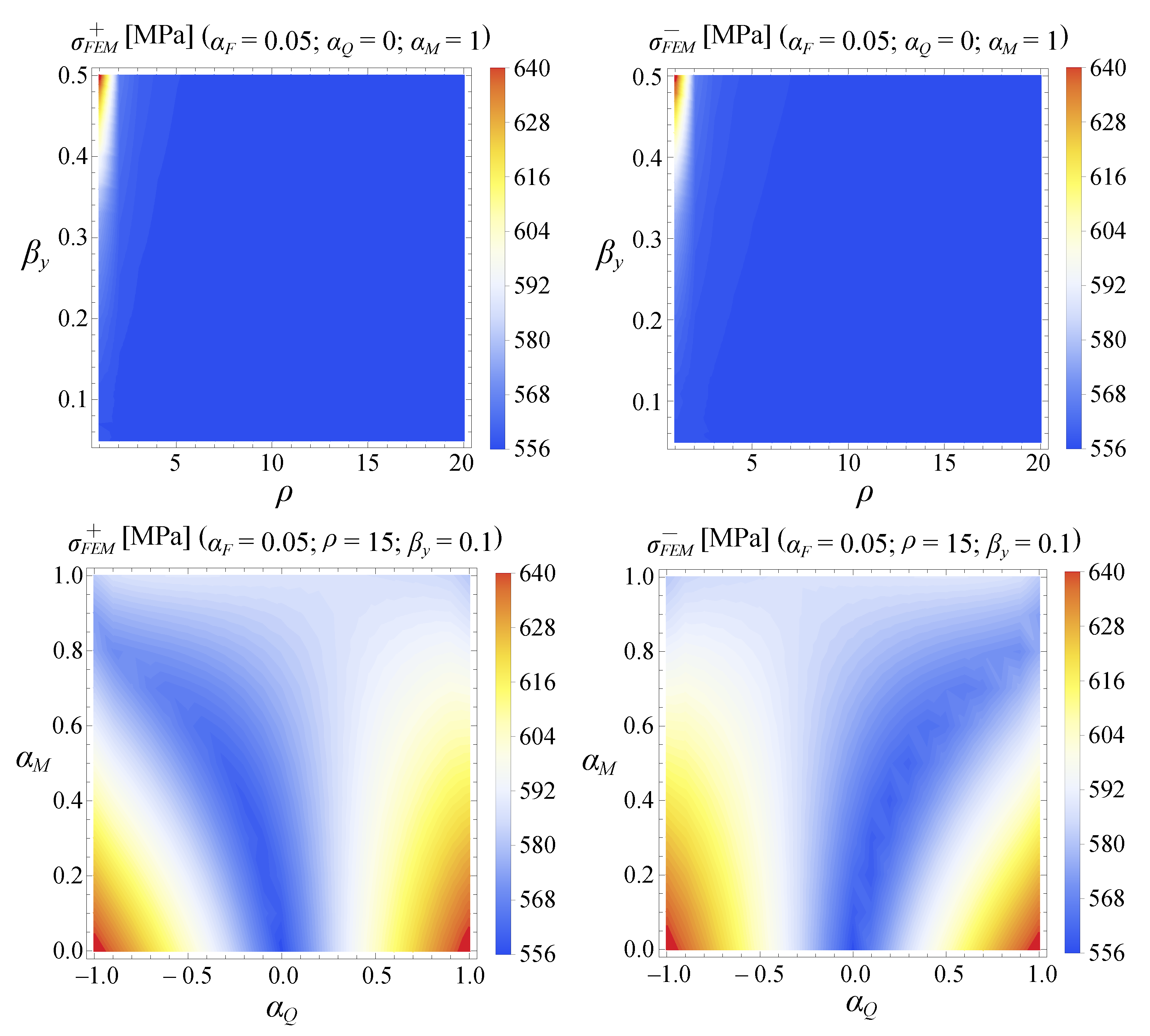
In Figure 16, the values of the maximum tension $\sigma$ in the flexure hinge are shown for different geometries (varying $\rho$ and ${\beta }_y$) and different load conditions (varying ${\alpha }_Q$ and ${\alpha }_M$). In the first case, the value of tension is quite uniform for the different geometries. It increases greatly when ${\beta }_y$ increases and $\rho$ decreases. In the second case, it can be observed, as expected, that the value of stress is not uniform at the different load conditions. In particular, the stress increases for small values of ${\alpha }_M$ and when ${\alpha }_Q$, in absolute value, is close to 1.

Figure 16. CASE III—Trend of the tension $\sigma$ evaluated by FE simulations varying $\rho$ and ${\beta }_y$ (up) and ${\alpha }_Q$ and ${\alpha }_M$ (down).

To summarize, tables and figures in all the proposed case studies provide information about the effect of geometric parameters in the kinematic behavior of a flexure joint, showing the importance of a proper stiffness model that will be required to move it accurately.

Nonlinear models can be typically avoided when small axial forces are applied to the free end of the flexure hinge, whereas the differences between the FE model and the linear analytical model become relevant when more important axial forces are involved.

On the contrary, it is evident from the proposed results that the linearization due to small rotations and the neglection of the term due to the axial deformation are both noninfluential contributions, at least for the typical rotation range allowed to flexure hinges. Their removal from the model is then allowed with the aim of obtaining a solvable formulation in analytical form. A linear model with an analytical solution is, therefore, the best choice in case axial forces have limited values.

7. Conclusions

In this work, the nonlinear bending model derived from continuum mechanics, which describes the rotational behavior of a flexure hinge under static loads, is analyzed.

The process of developing the model from nonlinear to linear through successive simplifications is presented in detail, showing the analytical solution of the latter and its conditions of applicability.

The present work shows how the approximated analytical model may be used to describe the angular displacement of the free-loaded end of an elliptical flexure hinge, also showing its limits of applicability with respect to the conventional complete model, which can only be solved in numerical form.

In particular, the axial force applied to the free end of the flexure hinge is shown to be the determining effect in choosing the reference stiffness model.

The introduction of some nondimensional parameters related to the geometry of the flexure hinge and the planar loads applied to its free end allows the evaluation of the angular displacements of the joint in different working conditions. As a result, it can be observed that the analytical model approximates the numerical one the better; the lower ${\alpha }_F$ and ${\alpha }_Q$ are in absolute value while having high values for ${\alpha }_M$. Regarding the geometric parameters, instead, the analytical model better approximates the behavior of the flexure hinge when ${\beta }_y$ decreases, namely when thin sections are chosen with respect to the overall height of the joint.

References

- Howell, L.L. Compliant Mechanisms; John Wiley & Sons: Hoboken, NJ, USA, 2001. [Google Scholar]
- Wang, P.Y.; Xu, Q.S. Design and Modeling of Constant-Force Mechanisms: A Survey. Mech. Mach. Theory 2018, 119, 1–21. [Google Scholar] [CrossRef]
- Oh, Y.S.; Kota, S. Synthesis of Multistable Equilibrium Compliant Mechanisms Using Combinations of Bistable Mechanisms. ASME J. Mech. Des. 2009, 131, 021002. [Google Scholar] [CrossRef]
- Kota, S.J.; Joo, Z.L.; Rodgers, S.M.; Sniegowski, J. Design of Compliant Mechanisms: Applications to MEMS. Analog Integr. Circuits Signal Process. 2001, 29, 7–15. [Google Scholar] [CrossRef]
- Qin, Y.D.; Shirinzadeh, B.; Tian, Y.L.; Zhang, D.W.; Bhagat, U. Design and Computational Optimization of a Decoupled 2-DOF Monolithic Mechanism. IEEE/ASME Trans. Mechatron. 2014, 19, 874–883. [Google Scholar] [CrossRef]
- Fleming, A.J.; Yong, Y.K. An Ultrathin Monolithic XY Nanopositioning Stage Constructed From a Single Sheet of Piezoelectric Material. IEEE/ASME Trans. Mechatron. 2017, 22, 2611–2618. [Google Scholar] [CrossRef]
- Xu, Q.S. Design and Development of a Novel Compliant Gripper With Integrated Position and Grasping/Interaction Force Sensing. IEEE Trans. Autom. Sci. Eng. 2017, 14, 1415–1428. [Google Scholar] [CrossRef]
- Tanikawa, T.; Arai, T. Development of a Micro-Manipulation System Having a Two-Fingered Micro-Hand. IEEE Trans. Robot. Autom. 1999, 15, 152–162. [Google Scholar] [CrossRef]
- Rakuff, S.; Cuttino, J.F. Design and Testing of a Long-Range, Precision Fast Tool Servo System for Diamond Turning. Precis. Eng. 2009, 33, 18–25. [Google Scholar] [CrossRef]
- Han, Y.M.; Han, C.; Kim, W.H.; Seong, H.Y.; Choi, S.B. Control Performances of a Piezoactuator Direct Drive Valve System at High Temperatures With Thermal Insulation. Smart Mater. Struct. 2016, 25, 097003. [Google Scholar] [CrossRef]
- Granstrom, J.; Feenstra, J.; Sodano, H.A.; Farinholt, K. Energy Harvesting From a Backpack Instrumented With Piezoelectric Shoulder Straps. Smart Mater. Struct. 2007, 16, 1810. [Google Scholar] [CrossRef]
- Sun, X.Q.; Yang, B.T. A New Methodology for Developing Flexure-Hinged Displacement Amplifiers With Micro-Vibration Suppression for a Giant Magnetostrictive Micro Drive System. Sens. Actuators A 2017, 263, 30–43. [Google Scholar] [CrossRef]
- Odhner, L.U.; Dollar, A.M. The Smooth Curvature Model: An Efficient Representation of Euler–Bernoulli Flexures as Robot Joints. IEEE Trans. Robot. 2012, 28, 761–772. [Google Scholar] [CrossRef]
- Paros, J.; Weisbord, L. How to design flexure hinge. Mach. Des. 1965, 37, 151–156. [Google Scholar]
- Smith, S.; Badami, V.; Dale, J.; Xu, Y. Elliptical flexure hinges. Rev. Sci. Instrum. 1997, 68, 1474–1483. [Google Scholar] [CrossRef]
- Lobontiu, N.; Paine, J.; Garcia, E.; Goldfarb, M. Corner-filleted flexure hinges. J. Mech. Des. 2001, 123, 346–352. [Google Scholar] [CrossRef]
- Lobontiu, N.; Paine, J.S.N.; O’Malley, E.; Samuelson, M. Parabolic and hyperbolic flexure hinges: Flexibility, motion precision and stress characterization based on compliance closed-form equations. Precis. Eng. 2002, 26, 183–192. [Google Scholar] [CrossRef]
- Tian, Y.; Shirinzadeh, B.; Zhang, D.; Zhong, Y. Three flexure hinges for compliant mechanism designs based on dimensionless graph analysis. Precis. Eng. 2010, 34, 92–100. [Google Scholar] [CrossRef]
- Tian, Y.; Shirinzadeh, B.; Zhang, D. Closed-form equations of the filleted V-shaped flexure hinges for compliant mechanism designs. Precis. Eng. 2010, 34, 408–418. [Google Scholar] [CrossRef]
- Chen, G.; Liu, X.; Gao, H.; Jia, J. A Generalized Model for Conic Flexure Hinges. Rev. Sci. Instrum. 2009, 80, 055106. [Google Scholar] [CrossRef]
- Lobontiu, N.; Cullin, M.; Ali, M.; Brock, J. A generalized analytical compliance model for transversely symmetric three-segment flexure hinges. Rev. Sci. Instrum. 2011, 82, 105116-1–105116-9. [Google Scholar] [CrossRef]
- Chen, G.M.; Jia, J.Y.; Li, Z.W. On Hybrid Flexure Hinges. In Proceedings of the 2005 IEEE Networking, Sensing and Control, Tucson, AZ, USA, 19–22 March 2005; pp. 700–704. [Google Scholar]
- Lin, R.; Zhang, X.; Long, X.; Fatikow, S. Hybrid flexure hinges. Rev. Sci. Instrum. 2013, 84, 085004. [Google Scholar] [CrossRef] [PubMed]
- Qi, K.Q.; Xiang, Y.; Fang, C.; Zhang, Y.; Yu, C.S. Analysis of the Displacement Amplification Ratio of Bridge-Type Mechanism. Mech. Mach. Theory 2015, 87, 45–56. [Google Scholar] [CrossRef]
- Ling, M.X.; Cao, J.Y.; Zeng, M.H.; Lin, J.; Inman, D.J. Enhanced Mathematical Modeling of the Displacement Amplification Ratio for Piezoelectric Compliant Mechanisms. Smart Mater. Struct. 2016, 25, 75022–75032. [Google Scholar] [CrossRef]
- Clark, L.; Shirinzadeh, B.; Pinskier, J.; Tian, Y.; Zhang, D. Topology Optimization of Bridge Input Structures With Maximal Amplification for Design of Flexure Mechanisms. Mech. Mach. Theory 2018, 122, 113–131. [Google Scholar] [CrossRef]
- Yong, Y.K.; Leang, K.K. Mechanical Design of High-Speed Nanopositioning Systems. In Nanopositioning Technologies; Springer: Cham, Switzerland, 2016; pp. 61–121. [Google Scholar]
- Lobontiu, N.; Paine, J.S.N.; Garcia, E.; Goldfarb, M.A. Design of Symmetric Conic-Section Flexure Hinges Based on Closed-Form Compliance Equations. Mech. Mach. Theory 2002, 37, 477–498. [Google Scholar] [CrossRef]
- Lyon, S.M.; Howell, L.L. A Simplified Pseudo-Rigid-Body Model for Fixed-Fixed Flexible Segments. In Proceedings of the International Design Engineering Technical Conferences and Computers and Information in Engineering Conference, Montreal, QC, Canada, 29 September–2 October 2002; ASME: New York, NY, USA, 2002; Volume 36533, pp. 23–33. [Google Scholar]
- Zhang, A.M.; Chen, G.M. A Comprehensive Elliptic Integral Solution to the Large Deflection Problems of Thin Beams in Compliant Mechanisms. ASME J. Mech. Robot. 2013, 5, 021006. [Google Scholar] [CrossRef]
- Wang, P.; Xu, Q.S. Design and Testing of a Flexure-Based Constant-Force Stage for Biological Cell Micromanipulation. IEEE Trans. Autom. Sci. Eng. 2018, 15, 1114–1126. [Google Scholar] [CrossRef]
- Ling, M.; Howell, L.; Cao, J.; Chen, G. Kinetostatic and dynamic modeling of flexure-based compliant mechanisms: A survey. Appl. Mech. Rev. 2020, 72, 030802. [Google Scholar] [CrossRef]
- Boyle, C.; Howell, L.L.; Magleby, S.P.; Evans, M.S. Dynamic Modeling of Compliant Constant-Force Compression Mechanisms. Mech. Mach. Theory 2003, 38, 1469–1487. [Google Scholar] [CrossRef]
- Li, Y.M.; Wu, Z.G. Design, Analysis and Simulation of a Novel 3-DOF Translational Micromanipulator Based on the PRB Model. Mech. Mach. Theory 2016, 100, 235–258. [Google Scholar] [CrossRef]
- Zhu, W.L.; Zhu, Z.; Guo, P.; Ju, B.F. A Novel Hybrid Actuation Mechanism Based XY Nanopositioning Stage With Totally Decoupled Kinematics. Mech. Syst. Signal Process. 2018, 99, 747–759. [Google Scholar] [CrossRef]
- Awtar, S.; Slocum, A.H. Closed-form nonlinear analysis of beam-based flexure modules. In Proceedings of the ASME International Design Engineering Technical Conferences and Computers and Information in Engineering Conference, Long Beach, CA, USA, 24–28 September 2005; pp. 101–110. [Google Scholar]
- Awtar, S.; Sen, S. A Generalized Constraint Model for Two-Dimensional Beam Flexures: Nonlinear Load-Displacement Formulation. ASME J. Mech. Des. 2010, 132, 081008. [Google Scholar] [CrossRef]
- Teo, T.; Chen, I.; Yang, G.; Lin, W. A generic approximation model for analyzing large nonlinear deflection of beam-based flexure joints. Precis. Eng. 2010, 34, 607–618. [Google Scholar] [CrossRef]
- Sen, S.; Awtar, S. A Closed-Form Nonlinear Model for the Constraint Characteristics of Symmetric Spatial Beams. ASME J. Mech. Des. 2013, 135, 031003. [Google Scholar] [CrossRef]
- Friedrich, R.; Lammering, R.; Heurich, T. Nonlinear modeling of compliant mechanisms incorporating circular flexure hinges with finite beam Elements. Precis. Eng. 2015, 42, 73–79. [Google Scholar] [CrossRef]
- Coffman, C.V. The Nonhomogeneous Classical Elastica; Technical Report; Department of Mathematics, Carnegie-Mellon University: Pittsburgh, PA, USA, 1976. [Google Scholar]
- Moschini, S.; Palpacelli, M.C. Practical range of applicability of a linear stiffness model of an elliptical flexure hinge. In Proceedings of the 2022 18th IEEE/ASME International Conference on Mechatronic and Embedded Systems and Applications (MESA), Taipei, Taiwan, 28–30 November 2022; pp. 1–6. [Google Scholar]
- Lenci, S.; Clementi, F.; Rega, G. Comparing nonlinear free vibrations of Timoshenko beams with mechanical or geometric curvature definition. Procedia IUTAM 2017, 20, 34–41. [Google Scholar] [CrossRef]
- Nayfeh, A.H.; Pai, P.F. Linear and Nonlinear Structural Mechanics; John Wiley & Sons: Hoboken, NJ, USA, 2008. [Google Scholar]
- Luongo, A.; Zulli, D. Mathematical Models of Beams and Cables; John Wiley & Sons: Hoboken, NJ, USA, 2013. [Google Scholar]
- Gerstmayr, J.; Irschik, H. On the correct representation of bending and axial deformation in the absolute nodal coordinate formulation with an elastic line approach. J. Sound Vib. 2008, 318, 461–487. [Google Scholar] [CrossRef]
- Lenci, S.; Rega, G. Nonlinear free vibrations of planar elastic beams: A unified treatment of geometrical and mechanical effects. Procedia IUTAM 2016, 19, 35–42. [Google Scholar] [CrossRef]
- Lenci, S.; Clementi, F.; Rega, G. A comprehensive analysis of hardening/softening behaviour of shearable planar beams with whatever axial boundary constraint. Meccanica 2016, 51, 2589–2606. [Google Scholar] [CrossRef]
- Babilio, E. Dynamics of an axially functionally graded beam under axial load. Eur. Phys. J. Spec. Top. 2013, 222, 1519–1539. [Google Scholar] [CrossRef]
- Chen, G.; Shao, X.; Huang, X. A new generalized model for elliptical arc flexure hinges. Rev. Sci. Instrum. 2008, 79, 095103. [Google Scholar] [CrossRef] [PubMed]
- Villaggio, P. Mathematical Models for Elastic Structures; Cambridge Univeristy Press: Cambridge, UK, 1997. [Google Scholar]
Disclaimer/Publisher’s Note: The statements, opinions and data contained in all publications are solely those of the individual author(s) and contributor(s) and not of MDPI and/or the editor(s). MDPI and/or the editor(s) disclaim responsibility for any injury to people or property resulting from any ideas, methods, instructions or products referred to in the content. |
© 2023 by the authors. Licensee MDPI, Basel, Switzerland. This article is an open access article distributed under the terms and conditions of the Creative Commons Attribution (CC BY) license (https://creativecommons.org/licenses/by/4.0/).