Anomaly Detection through Grouping of SMD Machine Sounds Using Hierarchical Clustering

Abstract

Surface-mounted device (SMD) assembly machines refer to production lines that assemble a variety of products that fit their purposes. As the required products become more diverse, models that oversee product anomaly detection are also becoming increasing linearly. In order to efficiently oversee products, the number of models has to be reduced and products with similar characteristics have to be grouped and overseen. In this paper, we show that it is possible to handle a large number of new products using latent vectors obtained from the autoencoder model. By hierarchically clustering latent vectors, the model finds product groups with similar characteristics and oversees them by group. Furthermore, we validate our multi-product operation strategy for anomaly detection with a newly collected SMD dataset. Experimental results show that the anomaly detection method using hierarchical clustering of latent vectors is a practical management method for SMD anomaly detection.

1. Introduction

SMD refers to a manufacturing line that continuously assembles various products. Two characteristics of SMDs are as follows:

• Continuity: The SMD assembly machine constantly assembles products along the manufacturing line, so if the manufacturing line breaks down, the damage is enormous.
• Product variety: The product type varies depending on which sensor is assembled, and the product type linearly increases over time.

There is a need for a system that can immediately detect abnormalities [1,2] when there is a problem in the manufacturing line; as products become linearly diversified, there is a need for a method that can effectively detect abnormalities in products.

Considering the real-world scenario, where a sufficient amount of abnormal data cannot be obtained, unsupervised learning, which trains only the normal data with the autoencoder [3,4,5] and detects the anomaly with the reconstruction error [6], is suitable.

Previous SMD anomaly detection studies [7,8,9] using autoencoder were developed as follows: Oh et al. [7] performed anomaly detection using a convolutional neural network (CNN)-based autoencoder. The anomaly detection performance of the proposed model was good, but in order to address the disadvantage of a long training time due to the many parameters to learn, Park et al. [8] proposed the fast adaptive RNN encoder–decoder (FARED). FARED is a recurrent neural network (RNN)-based anomaly detection model; it improves the anomaly detection performance while training faster and using fewer parameters than CNN. This is achieved using effective preprocessing methods and stacked RNNs. At that time, there were not many types of products, and the product assembly time was short and constant, so FARED did well in detecting abnormalities. As products diversified over time, two problems arose. One is that as the products diversified, the relatively short and constant assembly time became long and diverse, and the other problem is that there are too many models to manage. To address these problems, Nam et al. [9] proposed temporal adaptive average pooling (TAAP), which is a preprocessing method that enables more effective learning of longer and diversified assembly times, and self-attention based sequence-to-sequence autoencoder (SSS-AE), which can detect abnormalities in multiple products in one model while maintaining the advantage of a fast training speed. Although the multi-product anomaly detection performance of the SSS-AE model is robust, to oversee all products with one model, the products have become more diverse at this point, and there is a problem with having to train the model whenever a new SMD product is made. Therefore, we considered how to group and oversee products with relatively similar characteristics to reduce the number of models to be managed and the number of model trainings.

The proposed method is an anomaly detection technique based on the hierarchical clustering of latent vectors obtained through a pre-trained autoencoder. The autoencoder [3,4,5] is trained to represent data well in the latent space through the compression and reconstruction, and if the latent vectors obtained through the encoder of the pre-trained autoencoder have similar characteristics, the distances in the latent space will be closer than the data with different characteristics. Hierarchical clustering [10] is a system that groups objects into clusters based on their distance from individual clusters. In our proposed method, we leverage the characteristics of both autoencoder and hierarchical clustering to efficiently manage data by grouping them according to their similar features. First, we pre-train the autoencoder model with normal data from products that have abnormal data. The reason for pre-training with the normal data of products that include abnormal data is that abnormal data serve as the threshold for grouping data with similar features. Using a pre-trained autoencoder, we obtain latent vectors of the SMD data, and then perform hierarchical clustering based on the distances between the latent vectors in the latent space. Based on the distance between the latent vectors of the abnormal data and the latent vectors of the normal data of the products used for the pre-training, we group them if the distance between the latent vectors of the normal data of the products used for the pre-training and the latent vectors of the normal data of the other products is closer. The proposed method utilizes both autoencoder and clustering techniques to determine if the data exhibit similar features to the training data. By using abnormal data as the reference, if the data demonstrate similar characteristics, anomaly detection can be performed using the existing model without unnecessary training. This approach proves suitable for anomaly detection in SMD products, which are diverse and continuously produced. In this paper, we show that it is possible to group and oversee products with similar characteristics by hierarchically clustering the latent vector obtained from the autoencoder. Furthermore, we validate our proposed method with a newly collected SMD dataset.

2. Related Work

Our research covers both autoencoder and hierarchical clustering for anomaly detection. To facilitate the description of our research, we introduce existing autoencoder-based anomaly detection techniques and clustering-based anomaly detection techniques.

2.1. Autoencoder-Based Anomaly Detection

Chen et al. [11] proposed the convolutional autoencoder (CAE) [12] anomaly detection method and verified it with the NSL-KDD dataset [13], which consists of data selected from the KDD 99 dataset, which is an intrusion simulation dataset on the network. The convolution layer of the CAE that reduces the dimension of input data serves as an encoder, and the deconvolution layer of the CAE that reconstructs the reduced dimension serves as a decoder. This process can be expressed by the following equations:

$${\mathit{h}}^{\mathit{k}}=\sigma \left({\mathit{x}⊛{\mathit{W}}_x}^{\mathit{k}}+{\mathit{b}}_x^{\mathit{k}}\right),$$

(1)

$$\widehat{\mathit{x}}=\sigma \left(\sum _{k\in \mathit{H}}{\mathit{h}}^{\mathit{k}}⊛{\mathit{W}}_{\widehat{x}}^{\mathit{k}}+{\mathit{b}}_{\widehat{x}}^{\mathit{k}}\right),$$

(2)

where $\sigma$ refers to sigmoid, one of the activation functions, and ⊛ refers to the 2D convolution operation. $\mathit{k}$ refers to the number of feature maps of hidden representations, and $\mathit{W}$ and $b$ are the weights and biases of the convolution layer and the deconvolution layer. Chen et al. converted 1D data into 2D data by applying triangle area maps (TAMs) to apply the convolution autoencoder to 1D data; TAM converts each 1D vector $x=[x_0,x_1,\dots ,x_d]$ into a $\mathit{d}\times \mathit{d}$ matrix $\mathit{Y}$ according to the following equation: ${\mathit{y}}_{\mathit{ij}}=x_i\times x_j$, where $i,j\in [1,d]$. Said Elsayed et al. [14] proposed a method for anomaly detection in multivariate time series data using a long short-term memory (LSTM) [15]-based autoencoder. LSTM is a neural network that improves the gradient vanishing problem, which is a disadvantage of RNN, and is calculated in the following equations:

$${\mathit{i}}_{\mathit{t}}=\sigma ({\mathit{W}}_{\mathit{xi}}{\mathit{x}}_{\mathit{t}}+{\mathit{W}}_{\mathit{hi}}{\mathit{h}}_{\mathit{t}-\mathit{1}}+{\mathit{b}}_{\mathit{i}}),$$

(3)

$${\mathit{g}}_{\mathit{t}}=tanh({\mathit{W}}_{\mathit{xg}}{\mathit{x}}_{\mathit{t}}+{\mathit{W}}_{\mathit{hg}}{\mathit{h}}_{\mathit{t}-\mathit{1}}+{\mathit{b}}_{\mathit{g}}),$$

(4)

$${\mathit{f}}_{\mathit{t}}=\sigma ({\mathit{W}}_{\mathit{xf}}{\mathit{x}}_{\mathit{t}}+{\mathit{W}}_{\mathit{hf}}{\mathit{h}}_{\mathit{t}-\mathit{1}}+{\mathit{b}}_{\mathit{f}}),$$

(5)

$${\mathit{o}}_{\mathit{t}}=\sigma ({\mathit{W}}_{\mathit{io}}{\mathit{x}}_{\mathit{t}}+{\mathit{W}}_{\mathit{ho}}{\mathit{h}}_{\mathit{t}-\mathit{1}}+{\mathit{b}}_{\mathit{o}}),$$

(6)

$${\mathit{c}}_{\mathit{t}}={\mathit{f}}_{\mathit{t}}\circ {\mathit{c}}_{\mathit{t}-\mathit{1}}+{\mathit{i}}_{\mathit{t}}\circ {\mathit{g}}_{\mathit{t}},$$

(7)

$${\mathit{h}}_{\mathit{t}}={\mathit{o}}_{\mathit{t}}\circ tanh\left({\mathit{c}}_{\mathit{t}}\right),$$

(8)

where $x_t$ denotes the input at the time step t; $i_t$ and $g_t$ denote the input gates; $f_t$ and $o_t$ denote the forget and output gates; and $h_t$ and $c_t$ denote the hidden and cell states, respectively. Moreover, W, $b$, $\sigma$, and ∘ denote the weight matrices, bias vectors, the sigmoid function, and the Hadamard product (i.e., element-wise product), respectively. The encoder layer of the LSTM autoencoder compresses the multivariate time series input data $x_t$ = $[x_t^0,x_t^1,\dots ,x_t^{L-1}]$ into the hidden states of the encoder ${\mathit{h}}_{\mathit{t}}$ = $[{\mathit{h}}_{\mathit{t}}^{\mathit{0}},{\mathit{h}}_{\mathit{t}}^{\mathit{1}},\dots ,{\mathit{h}}_{\mathit{t}}^{\mathit{k}-\mathit{1}}]$ as follows:

$${\mathit{h}}_{\mathit{t}}=\mathit{LSTM}\left({\mathit{x}}_{\mathit{t}},{\mathit{h}}_{\mathit{t}-\mathbf{1}}\right),\mathit{z}=\mathit{f}\left({\mathit{h}}_{\mathit{t}}\right),$$

(9)

where t is the time step of input $\mathit{x}$, $\mathit{L}$ is the number of variables of input $x$, $\mathit{k}$ is smaller than $\mathit{L}$, $\mathit{f}$ is a non-linear function, and $\mathit{z}$ is the latent representation. The decoder layer reconstructs the latent representation $z$ to ${\widehat{\mathit{x}}}_{\mathit{t}}$ = $[{\widehat{x}}_t^0,{\widehat{x}}_t^1,\dots ,{\widehat{x}}_t^{L-1}]$ as follows:

$${\mathit{h}}_{\mathit{t}}^{\prime }=\mathit{LSTM}\left(\mathit{z},{\mathit{h}}_{\mathit{t}-\mathbf{1}}^{\prime }\right),{\widehat{\mathit{x}}}_{\mathit{t}}=\mathit{g}\left({\mathit{h}}_{\mathit{t}}^{\prime }\right),$$

(10)

where ${\mathit{h}}_{\mathit{t}}^{\prime }$ is the hidden state of the decoder at time step $\mathit{t}$ and $\mathit{g}$ is the non-linear function. Said Elsayed et al. used the sum of squared errors (SSEs) to calculate the reconstruction error.

2.2. Clustering-Based Anomaly Detection

Clustering is a method of grouping objects in the same group so that they are more similar than those in other groups [16]. Clustering techniques used for anomaly detection include fuzzy c-means clustering (FCM) [17], K-means clustering [18], and hierarchical clustering [10]. Shi et al. [19] demonstrated that hierarchical clustering was superior by comparing hierarchical clustering with k-means clustering and FCM, which are the most popular clustering techniques in anomaly detection, using the scientific data HTRU2 dataset [20] and tensile test dataset. Shi et al. [19] purposed improved agglomerative hierarchical clustering (IAHC), which dynamically adjusts the clustering linkage modes and the number of clusters during the hierarchical clustering algorithm iterations. The IAHC selects the optimal clustering distance linkage mode by comparing the Cophenetic correlation coefficient $\mathit{c}$ [21] calculated using Equation (11), considering single, complete, average, and centroid for each iteration of the algorithm. The Cophenetic correlation coefficient measures the similarity between individuals according to the following equation:

$$\mathit{c}=\frac{{\sum }_{i<j}[\mathit{x}(\mathit{i},\mathit{j})-\overline{\mathit{x}}][\mathit{t}(\mathit{i},\mathit{j})-\overline{\mathit{t}}]}{\sqrt{{\sum }_{i<j}{[\mathit{x}(\mathit{i},\mathit{j})-\overline{\mathit{x}}]}^2{\sum }_{i<j}({[\mathit{t}(\mathit{i},\mathit{j})-\overline{\mathit{t}}]}^2}}.$$

(11)

Suppose that the data ${\mathit{X}}_{\mathit{i}}$ have been modeled using a clustering method to produce a dendrogram ${\mathit{T}}_{\mathit{i}}$, where $\mathit{x}(\mathit{i},\mathit{j})$ is the Euclidean distance between the $\mathit{i}$th and $\mathit{j}$th observations, and $\mathit{t}(\mathit{i},\mathit{j})$ is the dendrogrammatic distance (i.e., Cophenetic distance) between the model points ${\mathit{T}}_{\mathit{i}}$ and ${\mathit{T}}_{\mathit{j}}$. $\overline{\mathit{x}}$ and $\overline{\mathit{t}}$ are the average of $\mathit{x}(\mathit{i},\mathit{j})$ and $\mathit{t}(\mathit{i},\mathit{j})$, respectively. If the optimal clustering distance mode is selected by comparing the Cophenetic correlation coefficient, we find the optimal clustering number. To find the optimal number of clusters, we assume the number of $\mathit{n}$ clusters in the optimal clustering distance mode, iterate algorithm m− 1 time, and then evaluate it as the criterion ${\mathit{e}}_{\mathit{n}}$. The range of $\mathit{n}$ follows $n\in [2,m]$, where $\mathit{m}$ is the maximum number of clusters of testing data according to domain knowledge. During the iteration of the algorithm $\mathit{m}-\mathit{1}$ time, the average number of samples of the smallest cluster in each result is taken as the threshold $\mathit{T}$. When the number of clusters is $\mathit{n}$, we denote the number of samples in cluster $\mathit{i}$ as ${\mathit{k}}_{\mathit{ni}}$ where $i=1,2,\dots ,n$. If ${\mathit{k}}_{\mathit{ni}}$ is less than the threshold $\mathit{T}$, we set $l_i=1$; otherwise, $l_i=0$. Then, ${\mathit{L}}_{\mathit{n}}$ and centroid ${\mathit{c}}_{\mathit{ni}}$ of the sample in each cluster is as follows:

$${\mathit{L}}_{\mathit{n}}=\sum _{i=1}^n{l}_i,{\mathit{c}}_{\mathit{ni}}=\frac{1}{k_{ni}}\sum _{h=1}^{k_{ni}}{x}_h,$$

(12)

where $x_h$ represents the sample of the cluster $\mathit{i}$, $h\in [1,k_{ni}]$.

The average distance of the centroids of clusters is calculated as follows:

$${\mathit{V}}_{\mathit{n}}=\frac{2}{n(n-1)}\sum _{j=i+1}^{n-1}d\left(c_{ni}-c_{nj}\right),$$

(13)

where $\mathit{i}\in [\mathit{1},\mathit{n}]$. Looking at criterion ${\mathit{e}}_{\mathit{n}}$ composed by ${\mathit{L}}_{\mathit{n}}$ and ${\mathit{V}}_{\mathit{n}}$, the optimum cluster number is the corresponding $\mathit{n}$ with the maximum ${\mathit{e}}_{\mathit{n}}$ calculated by the following equation:

$${\mathit{e}}_{\mathit{n}}=\frac{L_n}{{\sum }_{o=2}^m{L}_o}+\frac{V_n}{{\sum }_{o=2}^m{V}_o}.$$

(14)

Autoencoder-based anomaly detection techniques [11,14] introduced in Section 2.1 and clustering-based anomaly detection techniques [19] introduced in Section 2.2 are appropriate research studies for each task. However, it is not suitable to apply it to our tasks where data with new features keep increasing over time. If we apply an anomaly detection technique based on the autoencoder, we need to train the model every time new data are added; if we apply an anomaly detection technique based on clustering, domain knowledge can affect the performance; therefore, the criteria for clustering may be ambiguous. Our proposed anomaly detection technique is a method of grouping products with similar data characteristics using autoencoder and hierarchical clustering for effective management.

3. Proposed Method

In Section 3, we will describe the proposed method. The method utilizes hierarchical clustering of latent vectors obtained from a pre-trained autoencoder to establish clustering criteria based on the presence of two types of actual abnormal data. This approach effectively reduces the number of unnecessary models and training iterations. The encoder of the autoencoder is trained to accurately represent the features of the training data in the latent space. Consequently, when obtaining latent vectors of data using a pre-trained autoencoder, data with similar characteristics to the training data exhibit shorter distances in the latent space, while data with different characteristics exhibit longer distances. To leverage these characteristics, we propose a method that involves pre-training an autoencoder model with normal data containing abnormal data, performing hierarchical clustering using the obtained latent vectors, and grouping and managing data with similar characteristics. By employing hierarchical clustering, we use the distance between the latent vector of the training data and the latent vector of abnormal data as the threshold for grouping. If the latent vector of normal data from untrained products falls within this threshold, they are grouped. However, if it exceeds the threshold, individual models are trained for anomaly detection. Figure 1 shows the flowchart of the proposed method. Pre-training of the autoencoder is described in detail in Section 3.1 and hierarchical clustering in Section 3.2.

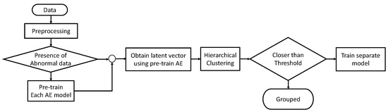
Figure 1. The flowchart of the proposed method.

3.1. Pre-Training the Autoencoder Model

Before explaining the pre-training of the autoencoder model, we introduce the autoencoder. The autoencoder [3] is a neural network that uses unsupervised learning algorithms to train so that the output is equal to the input. The autoencoder consists of an encoder that encodes a high-dimensional input $x=[x_0,x_1,\dots ,x_{n-1}]$ into a low-dimensional hidden representation $h=[h_0,h_1,\dots ,h_{d-1}]$ and a decoder that reconstructs the low-dimensional hidden representation $h$ to a high-dimensional $\widehat{x}=[{\widehat{x}}_0,{\widehat{x}}_1,\dots ,{\widehat{x}}_{n-1}]$. The equations for the encoder and decoder networks are as follows:

$$\mathit{h}=f\left({\mathit{W}}_{\mathit{h}}\mathit{x}+{\mathit{b}}_{\mathit{h}}\right),$$

(15)

$$\widehat{\mathit{x}}=g\left({\mathit{W}}_{\widehat{\mathit{x}}}\mathit{h}+{\mathit{b}}_{\widehat{\mathit{x}}}\right),$$

(16)

where $\mathit{x},\widehat{\mathit{x}}$∈${\mathit{R}}^{\mathit{n}}$, $\mathit{n}$ is the dimension of the input $\mathit{x}$ and output $\widehat{\mathit{x}}$, and $\mathit{h}$∈${\mathit{R}}^{\mathit{d}}$, ${\mathit{W}}_{\mathit{h}}$∈${\mathit{R}}^{\mathit{d}\times \mathit{n}}$, ${\mathit{W}}_{\widehat{\mathit{x}}}$∈${\mathit{R}}^{\mathit{n}\times \mathit{d}}$, $\mathit{d}$ is the dimension of the hidden representation $\mathit{h}$; $\mathit{W}$ and $\mathit{b}$ denote the weights and bias vectors, and $\mathit{f}$, $\mathit{g}$ are non-linear activation functions [22]. The autoencoder is trained by reducing the reconstruction error by Equations (17) and (18) between the input $x$ and the output $\widehat{x}$. If the input is continuous, we calculate the reconstruction error with the mean squared error in the following equation:

$$\mathcal{L}(x,\widehat{x})={∥x-\widehat{x}∥}^2,$$

(17)

If the input is categorical, we calculate the cross-entropy loss using the following equation:

$$\mathcal{L}(x,\widehat{x})=-\frac{1}{n}\sum _{i=1}^n(x_{\mathit{i}}log{\widehat{x}}_{\mathit{i}}+(1-x_{\mathit{i}})log(1-{\widehat{x}}_{\mathit{i}})),$$

(18)

where $\mathit{n}$ is the number of categories of categorical data. In the process of compressing and reconstructing the input data, the encoder of the autoencoder is trained to extract important features from the input data so that the decoder can accurately reconstruct the hidden representation.

We pre-train the model SSS-AE [9] to utilize the characteristics of the autoencoder. The SSS-AE is one of the autoencoder-based SMD anomaly detection models and has the best performance among existing SMD anomaly detection models, meaning that the model represents the input well in the latent space. The SSS-AE is a Seq2Seq-based autoencoder model, and RNN layers of the SSS-AE are LSTM. The encoder and decoder of the SSS-AE consist of $\mathit{N}$ blocks, consisting of LSTM, multi-head self-attention of the transformer [23], and layer normalization [24] being sequentially connected. The residual connection [25] is used to add the output of each sub-layer of the block before layer normalization. The last block of the decoder consists of one LSTM layer for reconstructing the output of the previous block as input.

We pre-train SSS-AE using normal data from products that contain abnormal data according to Algorithm 1. This is because abnormal data will be a threshold for finding untrained data with characteristics similar to those trained. Then, we obtain latent vectors for abnormal data of the trained product and normal data of untrained products using the pre-trained SSS-AE model.

Algorithm 1:Pre-trained autoencoder model with normal data

Input: Normal dataset $[x^0,x^1,\dots ,x^{n-1}]$ of the product,

where $\mathit{n}$ is the number of product data samples

Output: Encoder of the autoencoder

repeat

calculate $L(X,\widehat{X})$ by Equations (9), (10), and (17),

where $X$ is a set of data samples $x$ and $\widehat{X}$ denotes the output sequence data.

update parameter using gradients of $L$.

until epochs given in the experiment.

3.2. Hierarchical Clustering

By hierarchically clustering the obtained latent vectors according to the distance in the latent space, products closer than the distance between the normal data of the trained product and abnormal data $\mathit{Error}$ 1 and $\mathit{Error}$ 2 of the trained product can be grouped and overseen. $\mathit{Error}$ 1 is noise that is difficult for humans to distinguish, and $\mathit{Error}$ 2 is noise that can be recognized by humans.

Hierarchical clustering is a hierarchical system in which all objects are grouped into a single cluster, with each object represented as a separate cluster [10]. The following linkage methods [26] are used to compute the distance between two clusters $\mathit{U}$ and $\mathit{V}$. $\mathit{d}(\mathit{U},\mathit{V})$ refers to the distance between clusters $\mathit{U}$ and $\mathit{V}$.

• Centroid: For all combinations of data $u_i$ in cluster $\mathit{U}$ and data $v_j$ in cluster $\mathit{V}$, the distance between the center points of clusters $\mathit{U}$ and $\mathit{V}$ according to the following equation:

  $$\mathit{d}(\mathit{U},\mathit{V})={∥{\mathit{c}}_u-{\mathit{c}}_v∥}^2,$$

  (19)

  where ${\mathit{c}}_u$ and ${\mathit{c}}_v$ are the central points of the two clusters $\mathit{U}$ and $\mathit{V}$, respectively. The center point of the cluster uses the average of all data contained in the cluster according to the following equation:

  $${\mathit{c}}_{\mathit{u}}=\frac{1}{\left|\mathit{U}\right|}\sum _{\mathit{i}}{\mathit{u}}_{\mathit{i}},$$

  (20)

  where the $\left|\right|$ symbol refers to the number of elements in a cluster.
• Single: For all combinations of data ${\mathit{u}}_i$ and data ${\mathit{v}}_j$, we measure the distance to find the smallest value according to the following equation:

  $$d(\mathit{U},\mathit{V})=min\left(d({\mathit{u}}_i,{\mathit{v}}_j)\right).$$

  (21)
• Complete: For all combinations of data ${\mathit{u}}_i$ and ${\mathit{v}}_j$, we measure the distance to find the largest value according to the following equation:

  $$d(\mathit{U},\mathit{V})=max\left(d({\mathit{u}}_i,{\mathit{v}}_j)\right).$$

  (22)
• Average: For all combinations of data ${\mathit{u}}_i$ and ${\mathit{v}}_j$, we measure the distance to find the average according to the following equation:

  $$d(\mathit{U},\mathit{V})=\sum _{\mathit{i},\mathit{j}}\frac{d({\mathit{u}}_i,{\mathit{v}}_j)}{\left|\mathit{U}\right|\left|\mathit{V}\right|}.$$

  (23)
• Median: This method is a variation of the centroid linkage method. Similar to the centroid method, the distance of the center points of clusters is the distance between clusters. If clusters $\mathit{S}$ and $\mathit{T}$ combine to form cluster $U$ according to the following equation:

  $$\mathit{U}\leftarrow \mathit{S}+\mathit{T},$$

  (24)

  the center point of the cluster $\mathit{U}$ is not newly calculated, but the average of the center points of the two clusters of the original cluster is used according to the following equation:

  $${\mathit{c}}_{\mathit{u}}=\frac{1}{2}({\mathit{c}}_{\mathit{s}}+{\mathit{s}}_{\mathit{t}}).$$

  (25)
  Therefore, the calculation is faster than obtaining the center point by averaging all the data in the cluster.

The dendrogram resulting from the hierarchical clustering of the latent vectors can be used to set a threshold distance between the latent vectors of normal data and abnormal data of the trained product. Normal data of untrained products that are closer than this threshold can be grouped for anomaly detection. This is because the pre-trained autoencoder embeds data with similar characteristics to the training data closely in the latent space. By performing hierarchical clustering on these latent vectors, similar characteristics to the training data can be grouped together, which enables anomaly detection without the need for separate model training. If the grouping threshold is placed on $\mathit{Error}$ 1, it can be overseen more strictly, even though there are fewer products that can be grouped, and if the grouping threshold is placed on $\mathit{Error}$ 2, there are many products that can be grouped, so it can be overseen more efficiently.

4. Experiment

In this section, we describe the dataset in Section 4.1, the experimental process in Section 4.2, and the experimental results in Section 4.3. Section 4.1 describes the dataset used in the experiment and newly collected data for verification of the proposed method, and Section 4.1.1 describes how to preprocess the data to train the model more effectively before training it. Section 4.2 describes how the proposed method described in Section 3 was applied to the experiment, and Section 4.3 describes the experimental results.

4.1. Dataset

The SMD dataset consists of sound data collected by microphones installed on SMD assembly machines. As the SMD machine continuously assembles the product, the raw data represent the continuous assembly sounds of the product. As the raw data were too long for training, the data were segmented based on the assembly section of each individual product during the data collection process. The data collection process is the same as in the previous studies [7,8,9]. Figure 2 shows an example of the data collection process. In a previous study [9], we collected 30 normal data samples and 6 abnormal data samples. According to the characteristics of SMD products, which are diversified according to the combination of sensors, products are becoming more diversified in the real field. We collected 15 sets of normal data and 5 sets of abnormal data from 15 SMD products, and the new SMD dataset size is 6.1 GB. Abnormal data were actually collected when there was a problem in the assembly process and classified into two categories based on the degree of human recognition. These two error levels are expressed as Error 1 and Error 2, and are marked as product name-1 and product name-2. Since there are many types of products and the names are complicated, the first two letters of the product name, with one letter in alphabetical order, are combined and marked in the Abbr. column in the table. Amt. is the abbreviation for amount; the Amt. column in the table represents the number of samples collected for each respective product’s data. The previously collected dataset is described in Table 1 and the newly collected dataset is described in Table 2. The bold text in the table means abnormal.

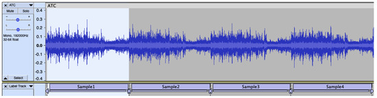
Figure 2. Example of the sound data collection process. Each sample is the assembly sound datum divided by the standard when the assembly of one product was completed.

Table 1. Large SMD dataset consisting of 30 normal products and 6 abnormal products. Bold text refers to abnormal products. Abnormal products were excluded from training.

Name	Abbr.	Time ($\mathit{\mu }$±$\mathit{\sigma }$ s)	Amt.	Name	Abbr.	Time ($\mathit{\mu }$±$\mathit{\sigma }$ s)	Amt.
AT2−AB	ATA	40.3 ± 2.1	100	NA−9473	NAB	13.1 ± 0	53
AT2−IN88	ATB	8.3 ± 0	63	RT−12DF	RTA	36.6 ± 0.9	29
C−SERIES	CSA	12. ± 0.8	41	ST−2524	STA	20.3 ± 0.7	46
CLR−085	CLA	34 ± 3.5	51	ST−2624	STB	19.5 ± 0.8	43
CT−C112B	CTA	45.4 ± 3.6	22	ST−2744	STC	17.4 ± 0.6	76
CT−C112T	CTB	40.1 ± 0.9	24	ST−3424	STD	25.9 ± 3.5	81
CT−C121B	CTC	33.9 ± 7.7	18	ST−3214	STE	26.8 ± 1.5	108
CT−C134B	CTD	44.4 ± 14.4	33	ST−3214−1	STE−1	27 ± 1.2	100
CT−C134T	CTE	34.5 ± 2.9	44	ST−3214−2	STE−2	27.5 ± 0.9	100
GT−3214	GTA	28.3 ± 2.6	33	ST−3428	STF	30.3 ± 2.7	89
GT−5112	GTB	25.6 ± 1.7	51	ST−3624	STG	28.5 ± 3.6	77
GW−9XXX	GWA	20.8 ± 2.1	93	ST−3704	STH	27.9 ± 1.5	64
GT−4118	GTC	35.9s ± 4.1	43	ST−3708	STI	40 ± 2.9	64
GT−4118−1	GTC−1	33.9 ± 3.3	14	ST−3708−1	STI−1	31 ± 2.1	35
GT−4118−2	GTC−2	28.4 ± 2.7	100	ST−3708−2	STI−2	36 ± 7.4	82
HV−M1230C	HVA	49.8 ± 2.6	39	ST−3804	STJ	25.2 ± 1.3	83
MG−A121H	MGA	30.1 ± 2	68	ST−7111	STK	8.7 ± 0.9	30
NA−9289	NAA	10.5 ± 0.1	55	TSIO−2002	TSA	19.8 ± 0.7	65

Table 2. Newly acquired SMD dataset consisting of 15 normal products and 5 abnormal products. Bold text refers to abnormal products. Abnormal products were excluded from training.

Name	Abbr.	Time ($\mathit{\mu }$±$\mathit{\sigma }$ s)	Amt.	Name	Abbr.	Time ($\mathit{\mu }$±$\mathit{\sigma }$ s)	Amt.
AT2−IO	ATC	29.6 ± 1.0	10	GT−2328−1	GTG−1	21.5 ± 1.5	54
AT2−IO−1	ATC−1	34.3 ± 0.8	26	GT−2744	GTH	17.8 ± 1.7	12
AT2−IO−2	ATC−2	30.9 ± 1.6	35	GT−5102	GTI	24.8 ± 0.7	16
AT2−89	ATD	26.7 ± 1.4	55	NA−9111	NAC	29.8 ± 0.5	20
AT2−89−1	ATD−1	26.7 ± 0.2	38	ST−2748	STL	19.3 ± 0.7	63
GT−1238	GTD	23.5 ± 0.9	61	ST−3114	STM	24.1 ± 2.8	15
GT−1238−2	GTD−2	28.1 ± 2.1	6	ST−3118	STN	31.7 ± 0.9	67
GT−225F	GTE	31.2 ± 0.6	72	ST−3234	STO	27.3 ± 1.8	32
GT−226F	GTF	30.8 ± 0.7	23	ST−3544	STP	28.7 ± 0.9	19
GT−2328	GTG	21.7 ± 0.4	64	ST−4212	STQ	17.7 ± 0.9	35

4.1.1. Data Preprocessing

Before training the model, we transformed the data into spectrograms $s$, representing the data in the time-frequency domain. $s\in {\mathit{R}}^{\mathit{T}\times \mathit{D}}$, where $\mathit{T}$ is the length of the spectrogram and $\mathit{D}$ is the number of frequency bins. As shown in the Time column in Table 1, the lengths of the data vary, and the length $\mathit{T}$ of the converted spectrogram $\mathit{s}$ also varies. We use temporal adaptive average pooling (TAAP) [9], which is an effective data preprocessing method that can reduce the variable length $\mathit{T}$ to a target length $\mathit{L}$ using an adaptive kernel. TAAP is calculated as follows:

$$k=⌈\frac{T}{L}⌉,$$

(26)

$${\overline{s}}_j=\frac{1}{k}{\sum }_{i=j\times k}^{(j+1)\times k-1}{s}_i,$$

(27)

where the $\lceil \rceil$ symbol refers to the ceiling function, $j=0,1,\dots ,L-1$. $\mathit{T}$ is a multiple of $\mathit{L}$; otherwise, zero-padding is used for spectrogram $\mathit{s}$. By using TAAP, data corruption can be minimized, and since it can be reduced to a fixed length, the calculation speed is increased because the data are not truncated or padded when configuring the batch, and the model can be trained reliably. After TAAP, we normalize the sequence $\overline{s}$ by min–max normalization.

4.2. Experimental Process

The experimental process consists of the following four main steps, and we describe the experimental setup in detail.

• Step 1: Data preprocessing.

We transform all datasets described in Table 1 into a Mel spectrogram. The Hanning window was used, and the window size was set to 2048, the hop size to 512, and the Mel filter bank to 80 for the transform. Then, TAAP was applied with a target length of 32 according to Equations (26) and (27), and normalized to min–max normalization.

• Step 2: Train the autoencoder model.

Each SSS-AE model was trained with normal data from product data {GTC, STE, STI}, where abnormal data exist to obtain an encoder that can represent each product well in the latent space. Then, with a trained encoder, all normal data and abnormal data, i.e., $\mathit{Error}$ 1 and $\mathit{Error}$ 2 of the base product of the group, were embedded in the latent space. The batch size for pre-training was set to 64, the number of epochs was set to 5000, the number of heads for multi-head self-attention was set to 8, and the Adam optimizer [27] was used.

• Step 3: Hierarchical clustering.

The latent vectors, obtained by embedding the data from each product {GTC, STE, STI} into the latent space using the encoder of the trained model, were hierarchically clustered using the centroid linkage mode based on Equations (19) and (20).

• Step 4: Verification of newly collected data.

To validate our methodology, we verify it with the newly collected dataset. We find out how many products can be grouped and overseen without training, including the product group found through hierarchical clustering, and verify whether anomaly detection is possible with the abnormal data of the newly collected dataset.

4.3. Experiment Result

To verify how much normal products can be overseen with only one pre-trained model, we apply hierarchical clustering to the data from three products, i.e., {STE, STI, GTC}, having normal and abnormal sounds. Figure A1 summarizes the hierarchical clustering results on each latent vector obtained from SSS-AE. We denote the distance value merged with each of the abnormal products with $\mathit{Error}$ 1 as a magenta color dotted line and $\mathit{Error}$ 2 as a red dotted line. First, in the results of the hierarchical clustering, we found that the data numbers from normal products grouped into the same cluster under $\mathit{Error}$ 1 for product data {STE, STI, GTC} were 1, 6, and 2. In the case of $\mathit{Error}$ 2, 23, 26, and 30 can be overseen in the same cluster. $\mathit{Error}$ 2 has a relatively higher noise compared to $\mathit{Error}$ 1, and more products can be grouped and overseen in one cluster, but $\mathit{Error}$ 1, with relatively weak noise, is overseen, similar to a normal product. It is up to the user to decide whether to group and manage more products under strong noise, such as $\mathit{Error}$ 2, or group them under weak noise, such as $\mathit{Error}$ 1, and manage them in the same cluster. We set $\mathit{Error}$ 1 as a threshold and verified our methodology with newly collected SMD data. Figure A2 is the result of hierarchically grouping the products that can be grouped by the $\mathit{Error}$ 1 threshold of the trained product data {STI} and the products that can be grouped by the $\mathit{Error}$ 1 threshold among the newly collected data. The black label refers to the data collected previously, and the blue label refers to the newly collected data. The magenta label refers to abnormal data at the level of $\mathit{Error}$ 1, and the red label refers to abnormal data at the level of $\mathit{Error}$ 2. The left and center dendrograms are hierarchically clustered results with newly collected product data {GTD, NAC}, respectively, which involves the process of finding product data within the $\mathit{Error}$ 1 threshold among the newly collected data. The dendrogram at the right is a hierarchical clustering result that includes product data {GTD, NAC, GTD-2}, which shows that the proposed method works by hierarchically clustering products within the $\mathit{Error}$ 1 threshold among the newly collected data and their abnormal data. Normal data are grouped together with normal data, the existing $\mathit{Error}$ 1 level of abnormal data is then clustered hierarchically, and the newly collected $\mathit{Error}$ 2 level of abnormal product data {GTD-2} is clustered with abnormal product data {STI-2}. This shows that product data that can be grouped through hierarchical clustering were found, and anomaly detection was possible through actual abnormal data.

5. Conclusions

SMD refers to a machine used for assembling electronic components or semiconductors on electronic boards. Due to the characteristics of SMD, which is continuously assembled along the manufacturing line, a large loss can be prevented by immediately detecting an abnormality. The problem is that the types of SMD products produced according to the combination of electronic components and sensors vary, and accordingly, the number of anomaly detection models also increases linearly. To resolve these problems, in this work, we proposed a practical management method by clustering various products using the structural characteristics of an autoencoder. The method involves hierarchically clustering the latent vectors embedded in the encoder of the autoencoder, even with a strict threshold that can detect the $\mathit{Error}\mathit{1}$ noise level, which is difficult for humans to detect. With one model trained only on the base product, up to 7 untrained normal products can be grouped and overseen, and for more efficient management, up to 30 untrained products can be grouped and overseen if they are grouped with a threshold that can detect the $\mathit{Error}\mathit{2}$ noise level, which is relatively easy to detect. The findings suggest that our anomaly detection method allows for anomaly detection without the need to train individual anomaly detection models for each new SMD product, as long as the data of the new product exhibit similar characteristics to the previously training data. These results provide evidence that the proposed methodologies can effectively operate SMD anomaly detection models in real-world situations.

Our research employs a threshold using abnormal data, but it primarily trains on normal data for anomaly detection. With the passage of time, the SMD assembly machine is expected to undergo aging, which can lead to changes in data characteristics even when the machine operates normally. Currently, our anomaly detection research does not encompass changes in data characteristics caused by machine aging. However, we plan to conduct future research on anomaly detection to account for such changes.

References

- Chandola, V.; Banerjee, A.; Kumar, V. Anomaly detection: A survey. ACM Comput. Surv. (CSUR) 2009, 41, 1–58. [Google Scholar] [CrossRef]
- Chalapathy, R.; Chawla, S. Deep learning for anomaly detection: A survey. arXiv 2019, arXiv:1901.03407. [Google Scholar]
- Zhang, G.; Liu, Y.; Jin, X. A survey of autoencoder-based recommender systems. Front. Comput. Sci. 2020, 14, 430–450. [Google Scholar] [CrossRef]
- Han, J.; Liu, T.; Ma, J.; Zhou, Y.; Zeng, X.; Xu, Y. Anomaly Detection and Early Warning Model for Latency in Private 5G Networks. Appl. Sci. 2022, 12, 12472. [Google Scholar] [CrossRef]
- Elhalwagy, A.; Kalganova, T. Multi-Channel LSTM-Capsule Autoencoder Network for Anomaly Detection on Multivariate Data. Appl. Sci. 2022, 12, 11393. [Google Scholar] [CrossRef]
- Wulsin, D.; Blanco, J.; Mani, R.; Litt, B. Semi-supervised anomaly detection for EEG waveforms using deep belief nets. In Proceedings of the 2010 Ninth International Conference on Machine Learning and Applications, Washington, DC, USA, 12–14 December 2010; pp. 436–441. [Google Scholar]
- Oh, D.Y.; Yun, I.D. Residual error based anomaly detection using autoencoder in SMD machine sound. Sensors 2018, 18, 1308. [Google Scholar] [CrossRef]
- Park, Y.; Yun, I.D. Fast adaptive RNN encoder–decoder for anomaly detection in SMD assembly machine. Sensors 2018, 18, 3573. [Google Scholar] [CrossRef]
- Nam, K.H.; Song, Y.J.; Yun, I.D. SSS-AE: Anomaly Detection using Self-Attention based Sequence-to-Sequence Autoencoder in SMD Assembly Machine Sound. IEEE Access 2021, 9, 131191–131202. [Google Scholar] [CrossRef]
- Johnson, S.C. Hierarchical clustering schemes. Psychometrika 1967, 32, 241–254. [Google Scholar] [CrossRef] [PubMed]
- Chen, Z.; Yeo, C.K.; Lee, B.S.; Lau, C.T. Autoencoder-based network anomaly detection. In Proceedings of the 2018 Wireless Telecommunications Symposium (WTS), Phoenix, AZ, USA, 17–20 April 2018; pp. 1–5. [Google Scholar]
- Masci, J.; Meier, U.; Cireşan, D.; Schmidhuber, J. Stacked convolutional autoencoders for hierarchical feature extraction. In Proceedings of the International Conference on Artificial Neural Networks, Espoo, Finland, 14–17 June 2011; Springer: Berlin/Heidelberg, Germany, 2011; pp. 52–59. [Google Scholar]
- Tavallaee, M.; Bagheri, E.; Lu, W.; Ghorbani, A.A. A detailed analysis of the KDD CUP 99 dataset. In Proceedings of the 2009 IEEE Symposium on Computational Intelligence for Security and Defense Applications, Ottawa, ON, Canada, 8–10 July 2009; pp. 1–6. [Google Scholar]
- Said Elsayed, M.; Le-Khac, N.A.; Dev, S.; Jurcut, A.D. Network anomaly detection using LSTM based autoencoder. In Proceedings of the 16th ACM Symposium on QoS and Security for Wireless and Mobile Networks, Alicante, Spain, 16–20 November 2020; pp. 37–45. [Google Scholar]
- Hochreiter, S.; Schmidhuber, J. Long short-term memory. Neural Comput. 1997, 9, 1735–1780. [Google Scholar] [CrossRef] [PubMed]
- Diday, E.; Simon, J. Clustering analysis. In Digital Pattern Recognition; Springer: Berlin/Heidelberg, Germany, 1976; pp. 47–94. [Google Scholar]
- Izakian, H.; Pedrycz, W. Anomaly detection in time series data using a fuzzy c-means clustering. In Proceedings of the 2013 Joint IFSA World Congress and NAFIPS Annual Meeting (IFSA/NAFIPS), Edmonton, AB, Canada, 24–28 June 2013; pp. 1513–1518. [Google Scholar]
- Kumar, S.; Khan, M.B.; Hasanat, M.H.A.; Saudagar, A.K.J.; AlTameem, A.; AlKhathami, M. An Anomaly Detection Framework for Twitter Data. Appl. Sci. 2022, 12, 11059. [Google Scholar] [CrossRef]
- Shi, P.; Zhao, Z.; Zhong, H.; Shen, H.; Ding, L. An improved agglomerative hierarchical clustering anomaly detection method for scientific data. Concurr. Comput. Pract. Exp. 2021, 33, e6077. [Google Scholar] [CrossRef]
- Lyon, R.J.; Stappers, B.; Cooper, S.; Brooke, J.M.; Knowles, J.D. Fifty years of pulsar candidate selection: From simple filters to a new principled real-time classification approach. Mon. Not. R. Astron. Soc. 2016, 459, 1104–1123. [Google Scholar] [CrossRef]
- Saraçli, S.; Doğan, N.; Doğan, İ. Comparison of hierarchical cluster analysis methods by Cophenetic correlation. J. Inequalities Appl. 2013, 2013, 1–8. [Google Scholar] [CrossRef]
- Sharma, S.; Sharma, S.; Athaiya, A. Activation functions in neural networks. Towards Data Sci. 2017, 6, 310–316. [Google Scholar] [CrossRef]
- Vaswani, A.; Shazeer, N.; Parmar, N.; Uszkoreit, J.; Jones, L.; Gomez, A.N.; Kaiser, Ł.; Polosukhin, I. Attention is all you need. In Proceedings of the Advances in Neural Information Processing Systems, Long Beach, CA, USA, 4–9 December 2017; pp. 5998–6008. [Google Scholar]
- Ba, J.L.; Kiros, J.R.; Hinton, G.E. Layer normalization. arXiv 2016, arXiv:1607.06450. [Google Scholar]
- He, K.; Zhang, X.; Ren, S.; Sun, J. Deep residual learning for image recognition. In Proceedings of the IEEE Conference on Computer Vision and Pattern Recognition, Las Vegas, NV, USA, 27–30 June 2016; pp. 770–778. [Google Scholar]
- Murtagh, F.; Contreras, P. Algorithms for hierarchical clustering: An overview. Wiley Interdiscip. Rev. Data Min. Knowl. Discov. 2012, 2, 86–97. [Google Scholar] [CrossRef]
- Kingma, D.P.; Ba, J. Adam: A method for stochastic optimization. arXiv 2014, arXiv:1412.6980. [Google Scholar]
Disclaimer/Publisher’s Note: The statements, opinions and data contained in all publications are solely those of the individual author(s) and contributor(s) and not of MDPI and/or the editor(s). MDPI and/or the editor(s) disclaim responsibility for any injury to people or property resulting from any ideas, methods, instructions or products referred to in the content. |
© 2023 by the authors. Licensee MDPI, Basel, Switzerland. This article is an open access article distributed under the terms and conditions of the Creative Commons Attribution (CC BY) license (https://creativecommons.org/licenses/by/4.0/).