Detecting SPIT Attacks in VoIP Networks Using Convolutional Autoencoders: A Deep Learning Approach

Abstract

Voice over Internet Protocol (VoIP) is a technology that enables voice communication to be transmitted over the Internet, transforming communication in both personal and business contexts by offering several benefits such as cost savings and integration with other communication systems. However, VoIP attacks are a growing concern for organizations that rely on this technology for communication. Spam over Internet Telephony (SPIT) is a type of VoIP attack that involves unwanted calls or messages, which can be both annoying and pose security risks to users. Detecting SPIT can be challenging since it is often delivered from anonymous VoIP accounts or spoofed phone numbers. This paper suggests an anomaly detection model that utilizes a deep convolutional autoencoder to identify SPIT attacks. The model is trained on a dataset of normal traffic and then encodes new traffic into a lower-dimensional latent representation. If the network traffic varies significantly from the encoded normal traffic, the model flags it as anomalous. Additionally, the model was tested on two datasets and achieved F1 scores of 99.32% and 99.56%. Furthermore, the proposed model was compared to several traditional anomaly detection approaches and it outperformed them on both datasets.

1. Introduction

VoIP is a technology utilized for transmitting voice and multimedia information across Internet Protocol (IP) networks. The adoption of VoIP systems has been growing worldwide due to their cost-effectiveness and ability to provide high-quality voice and multimedia communication services. As fifth-generation (5G) networks emerge, VoIP is expected to become the dominant technology for voice communications.

The essential components of VoIP systems include end-user equipment, network components, call processors, gateways, and protocols. To facilitate the transfer of voice and multimedia data over packet-switched IP networks, VoIP systems employ data transfer protocols such as the Real-Time Transport Protocol (RTP) [1]. Furthermore, signaling protocols such as H.323 or the SIP [2] are utilized to manage communication sessions.

A vast number of people are progressively using VoIP in addition to the conventional public switched telephone network for commercial and personal purposes. Due to VoIP’s appealing low-cost international calls, the number of subscribers has dramatically increased in recent years. Additionally, VoIP offers value-priced services at a low cost and the freedom to use IP networks for voice communication. These advantages of VoIP services dramatically increase the number of their subscribers. According to the Cisco report, the number of networked devices will be about 29 billion by 2023 [3]. Meanwhile, VoIP users have become vulnerable to many attacks, such as SPIT detection [4]. SPIT is mostly used to promote items, annoy subscribers, induce users to call special numbers, or conduct vishing attempts to obtain private information from call participants [5].

Several researchers proposed a variety of SPIT detection strategies, as addressed in the next section. To our knowledge, anomaly detection has not been deployed before for detecting SPIT messages. Finding data instances that substantially differ from the majority of the dataset is the goal of anomaly detection techniques.

The classical anomaly detection approaches such as One-Class Support Vector Machine (OC-SVM) [6] and Kernel Density Estimation (KDE) [7] fail to obtain satisfactory performance in certain scenarios with high-dimensional data due to their limited computational scalability. To cope with these limitations, these classical approaches require significant feature engineering. However, deep learning anomaly detection methods can handle complicated data following the principle of learning efficient representations and training multi-layered neural networks using the data directly. Currently, the primary approaches to deep anomaly detection include autoencoders, one-class classification, and generative methods [8].

An autoencoder (AE) is an unsupervised neural network optimized so that its output copies its Aninput [9]. The area of unsupervised anomaly detection uses them frequently [10,11]. AEs learn relevant feature representations of their input. As shown in Figure 1, two phases make up the AE model: the encoder and the decoder. The encoder, represented as $H=f\left(X\right)$, is responsible for compressing the input X into a lower-dimensional latent representation H.

$$\begin{array}{c}\hfill H=f(WX+b)\end{array}$$

(1)

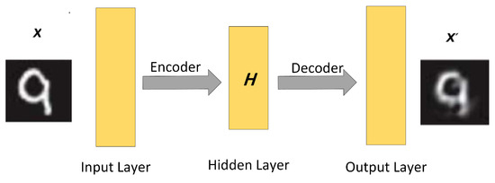
Figure 1. Autoencoder with one-layer encoder and one-layer decoder.

W and b in Equation (1) are the weight and bias vectors of the encoder, and f is a nonlinear activation function such as a sigmoid, tanh, or the rectified linear unit (ReLU) function. On the other hand, the decoder, represented as $X^{\prime }=g\left(H\right)$, attempts to reconstruct the original input X from the latent representation H, ultimately producing the output $X^{\prime }$.

$$\begin{array}{c}\hfill X^{\prime }=f(W^{\prime }H+b^{\prime })\end{array}$$

(2)

Similarly, $W^{\prime }$ and $b^{\prime }$ in Equation (2) are the weight and bias vectors of the decoder, and g is a nonlinear activation function similar to f. Throughout the training process, the AE’s parameters $\theta =\{W,W^{\prime },b,b^{\prime }\}$ are optimized by minimizing the reconstruction error, which is computed using a loss function.

In this paper, a novel method for detecting SPIT attacks in VoIP networks is proposed. The approach involves an end-to-end detection system that utilizes a deep learning autoencoder-based model to analyze Session Initiation Protocol (SIP) messages. Unlike traditional methods, this model does not require feature engineering to identify potential attacks. To our knowledge, the proposed model is the first of its kind to use autoencoders for this purpose. The primary contributions of this study include (1) introducing the One-Dimensional Deep Convolutional Autoencoder (1D-DCAE) as a new model for SPIT detection, (2) achieving high accuracy in detecting SPIT attacks across two different datasets, and (3) comparing the performance of the 1D-DCAE model with state-of-the-art classical machine learning methods.

The structure of this paper is as follows: The next section provides a comprehensive review of related research in the field. Section 3 presents the proposed method for identifying SPIT attacks in detail. Section 4 provides an overview of the two datasets used to evaluate the proposed model. Section 5 outlines the experimental setup, performance metrics, and results. Finally, the findings of the study and directions for future research are concluded in Section 6.

2. Related Work

Various approaches reported in the literature have used machine learning algorithms for detecting SPIT attacks in SIP-based VoIP networks. A large portion of these approaches focused on clustering and classifying network callers as spam and non-spam callers.

M. Azrour et al. [12] used the K-mean algorithm to cluster spam and non-spam callers. K-mean is an unsupervised clustering machine learning algorithm. Caller-selected features were used as input for the K-mean algorithm. Such features include call duration average, direction ratio, call ratio, call frequency, day’s calls ratio, and trusted callees. The experiments were conducted on a dataset comprising 6100 calls spanning 180 days. Three scenarios were tested, considering varying ratios of low and high spammers to normal callers. The results revealed a high F1 score for the high spammers to normal callers ratio, while a low F1 score was obtained for the low spammers to normal callers ratio.

M. Swarnkaret et al. [13] proposed the use of a directed weighted social graph that models the interaction among the network users. By examining the resemblance of a node (i.e., caller) to its nearby nodes in the graph, this node is categorized as an anomaly (i.e., spam caller) if it deviates from its neighbors. Caller-related parameters were used to calculate the weights on the edges of the graph. Three parameters, namely average talk time, successful call rate, and role in the call, were utilized. The identification of anomalies in the graph involves examining the local neighborhood of a node, with any node that appears distinct from its surroundings being categorized as an anomaly. To evaluate their approach, a Call Detail Record (CDR) of simulated callers, comprising both normal and spam users, was generated. The results demonstrated that their approach successfully detected 100% of spammers with 0% false positives.

Azad et al. [14] also deployed a weighted directed social graph to extract the social behavior of callers and their call patterns. They fed these features into a decision tree algorithm to classify a caller as a normal caller, center caller, or spam caller. A social graph was constructed using more than ten million call detail records provided by an anonymous telecommunication operator, which included data from two million users. By analyzing the graph, caller features were extracted for each class. Subsequently, a decision tree algorithm was trained using these features and the corresponding labels of each caller, allowing the construction of a classifier capable of categorizing callers into the three primary classes.

The reputation model developed by Javed et al. [4] was aimed at detecting spam callers in a network. The caller’s reputation was computed in a hybrid manner by considering call features such as call density, call duration, and call rate from CDRs as well as recommendations from reliable callers. Their approach also tries to whitewash by imposing restrictions on new network users. New users are allowed to conduct a limited number of calls in a certain time period and connect to a limited number of unique callees. This limits the ability of new users to generate spam calls. A new user must build a good reputation to become a “mature” user who is able to communicate freely. The authors used synthetic call data records that simulate the behaviors of the different caller types (i.e., a legitimate, spammer, telemarketer, and others). The results of this model demonstrated an increase in detection accuracy over time, stabilizing at 0.98. In addition, the behavior of the detection accuracy persists even when only 15% of the users report spammers.

Pereira et al. [15] proposed a framework to detect malicious SIP calls. Their framework is based on deep Recurrent Neural Networks (RNNs), specifically Long Short-Term Memory (LSTM) RNNs, in the initial stage. Additionally, a classifier based on “skewness and kurtosis” was developed as a second stage, which detects anomalous SIP dialogs. The features generated from the first stage LSTM RNN model are fed as input to the classifier. To evaluate the performance of their framework, the researchers conducted training and testing on the widely recognized INRIA dataset [16], which comprises both normal and anomalous SIP dialogs. The classifier achieved a detection accuracy of 99.84% on previously unseen SIP dialogs.

Oliveira et al. [17] proposed a framework to detect malicious SIP calls. The first stage of this framework was built using a deep Convolution Neural Network (CNN) [18]. The proposed model was compared to the LSTM RNN model proposed in [15]. Through a comparison between the two models, Oliveira et al. demonstrated the computational advantages of the CNN model over the LSTM RNN model, particularly in terms of complexity. This approach has a shorter detection time than the LSTM RNN model. In addition, a “maximum output-based” classifier was built as a second stage to detect anomalous SIP dialogs using the features generated by the first stage model (CNN or LSTM RNN). The classifier was trained on labeled data, which consists of normal and anomalous SIP dialogs, and then tested on unseen SIP dialogs in order to identify its detection performance. Interestingly, a comparison between the newly developed classifier and the previously utilized skewness-and-kurtosis-based classifier revealed that the latter outperformed the former in detecting anomalous SIP dialogs.

Nazih et al. [19] proposed a method for detecting Distributed Denial-of-Service (DDoS) attacks over VoIP using RNNs. Two techniques for feature extraction, namely token-based and character-based, were investigated, and it was reported that token-based feature extraction achieved a higher F1 score. The authors utilized a real dataset and injected it with DDoS messages of varying intensities. Their approach achieved a high F1 score for both low-rate and high-rate attacks.

Tas et al. [20] introduced a method to protect VoIP networks against advanced attacks that exploit less-known SIP features, specifically the SIP-based distributed reflection denial of service (SIP-DRDoS) attack. The proposed method included three modules: statistics, inspection, and action, which work together to identify and prevent attack packets. In addition, experimental evaluations were conducted within a VoIP/SIP security lab environment, involving the implementation of the SIP-DRDoS attack and the defense mechanism. The results showed that the defense mechanism was successful in detecting and mitigating the attack within 6 minutes of initiation, reducing the CPU usage of the SIP server from 74% to 17%.

Henry et al. [21] presented a new IDS development method that employs a CNN with a Gated Recurrent Unit (GRU). This combination was utilized to enhance network parameters and address the limitations associated with existing deep learning methods. In addition, the CICIDS dataset was optimized to reduce input size and features. The findings demonstrated a substantial increase in attack detection accuracy, with a 98.73% accuracy and a 0.075 FPR. Furthermore, the effectiveness of the proposed IDS model was compared to other existing techniques, and the results indicate its usefulness in real-world cybersecurity scenarios. This novel approach represented an important advancement in safeguarding organizational boundaries amid the growing number of IoT devices and increasing attack surfaces.

Kasongo et al. [22] used different types of RNNs to improve the security of network systems. The proposed framework consisted of three layers: data collection and processing, feature extraction, and model building. The first layer involved normalizing the dataset and applying the XGBoost algorithm to generate a vector containing feature importance values. Then, RNN-based classifiers were trained, validated, and tested independently. In addition, a detailed analysis of the different types of RNNs and the XGBoost algorithm used in the proposed framework was provided. Furthermore, the proposed IDS framework was implemented on two benchmark datasets (i.e., NSL-KDD, and the UNSW-NB15) and used an XGBoost-based feature selection algorithm to reduce the feature space of each dataset. The results showed that the XGBoost-RNN-based IDSs outperform existing methods and achieve high accuracy.

Chaganti et al. [23] proposed an LSTM-based approach for detecting network attacks using Software Defined Network (SDN) intrusion detection systems in IoT networks. The authors analyzed the performance of different deep learning architectures and classical machine learning models using two SDN-IoT datasets. The proposed model architecture consisted of 4 LSTM layers with 64 units, 4 dropout layers, and a dense layer. This architecture was shown to be effective in the binary and multiclass classification of network attacks. In addition, this LSTM model was found to be robust and generalizable to handle various SDN attacks. Furthermore, it effectively classifies the attack types with an accuracy of 0.971%.

3. Proposed Approach

The aim of the proposed approach is to utilize deep learning algorithms to construct One Dimensional Deep Convolutional Autoencoder (i.e., 1D-DCAE) model that can learn the features of normal SIP messages and identify any anomalies (i.e., SPIT attacks). The construction of this model involves two phases: the initial phase entails the extraction of relevant features from SIP messages, while the subsequent phase deploys the 1D-DCAE model for the detection of SPIT attacks.

3.1. Feature Extraction

The proposed approach for feature extraction is different from previous machine learning approaches for detecting VoIP attacks, as designing features that accurately represent messages is necessary [12,24]. Figure 2 illustrates the feature extraction process. It starts by tokenizing messages, padding them, and embedding them.

Figure 2. Stages of feature extraction: Tokening, Padding, and Embedding.

In the tokenizing step, all the words in the dataset are used to create a dictionary. Each SIP message produces a sequence of tokens, where a token is an index to a specific word in the dictionary. In the second step, zeros are padded to the end of every sequence to make all the sequences equal in length. The length of the sequences is selected as 104.

Word embedding [25] has shown remarkable performance in representing the semantic and syntactic characteristics of texts. It captures the resemblance of words (i.e., tokens) in a given dictionary. For the embedding step, a word embedding layer is employed as the first layer in the proposed model to map tokens from discrete to continuous embedded representation. Each token is mapped to an embedding vector of length 50. Therefore, each SIP message is converted to a $104\times 50$ feature map X, before being fed to the encoder part of the proposed model.

3.2. Autoencoder Reconstruction Error

An AE model is trained using data X. After the training process, the model is able to encode and output $X^{\prime }=g\left(H\right)$, a reconstructed version of X. If the model receives an input that differs from the training data, it cannot successfully reconstruct the input, leading to a high reconstruction error. Thus, AEs can be used to detect anomalies [26,27] by contrasting the reconstruction error against a predetermined threshold. The Mean Absolute Error (MAE) can be utilized as a loss function L to calculate the reconstruction error, as shown below:

$$\begin{array}{cc}\hfill L\left(\theta \right)& =\underset{\theta }{min}\frac{1}{2N}\parallel X-X^{\prime }\parallel \hfill \\ \hfill & =\underset{\theta }{min}\frac{1}{2N}\parallel X-g\left(f\left(X\right)\right)\parallel \hfill \end{array}$$

(3)

where N in Equation (3) is the number of training samples. This approach aims to discriminate SIP messages that contain SPIT attacks from normal ones.

3.3. Deep Convolutional Autoencoder (DCAE)

A Convolutional Autoencoder is a variant of an AE. The encoder part is implemented as a CNN [18] rather than a basic neural network, and the decoder part is implemented as a flipped CNN (i.e., deconvolutional layers instead of convolutional layers). In a CAE, the encoder is a multi-layer CNN (i.e., a deep CNN), and the decoder consists of a flipped deep CNN. Deep CNNs are very efficient at extracting features from multi-scale perspectives, from the bottom layer up to the top layer of the network. Therefore, DCAE [28] leverages the ability of the AE to attain a strong, relevant feature representation of the training data.

A Deep CNN mainly consists of convolution layers stacked over each other. A convolution layer applies a convolution operation between a filter called a “kernel” and its input. The kernel size is usually 3 × 3 and its weights are learned during the training process. Starting from the upper left of the input image (or a feature map from a previous layer), the kernel swipes through the whole input image, moving one position at a time (i.e., stride) and the convolution operation is repeated until the whole input image is covered. The result of this process is called a “feature map”. There are multiple kernels for each convolution layer, and all are randomly initialized. Therefore, a convolution layer outputs multiple feature maps. When a Graphics Processing Unit (GPU) is used, all of the aforementioned computations are executed simultaneously. Once feature maps are computed, each element in the feature maps is passed through the ReLU [29]. The ReLU is a piece-wise linear function that outputs the same input if it is positive and zero otherwise.

In order to downsample the feature maps, a pooling layer comes after a convolution layer in DCAE and many other CNN architectures. This downsampling is accomplished using either maximum or average pooling. Max-pooling sets the output value as the maximum value of the values covered by the pooling filter, whereas average-pooling calculates and outputs the average value. Similar to the convolution kernel in the convolution layer, the pooling filter moves one stride at a time and swipes through the whole feature map. The size of the pooling filter is usually 2 × 2. This results in reducing the length and width of feature maps by half.

3.4. The Architecture

The architecture of a DCAE for image reconstruction is built using two-dimensional (2D) multi-convolutional/deconvolutional layers with 2D feature maps because of the nature of the input data (i.e., a 2D image). Whereas, the architecture of a DCAE for sequential input data, such as text and electrocardiogram (ECG) data, is built using multi-one-dimensional (1D) convolutional/deconvolutional layers, i.e., the kernels and the feature maps are 1D. Each SIP message is a sequential text input; thus, in order to detect SPIT attacks in SIP messages, the proposed model was constructed using a D1-DCAE architecture.

3.5. D1-DCAE Model

The proposed D1-DCAE model, illustrated in Figure 3, comprises an embedding layer, an encoder consisting of three blocks, and a decoder consisting of another three blocks. Each encoder block comprises a convolutional layer with a 1 × 3 kernel and a stride of 1, followed by a max-pooling layer. The filter of the max-pooling layer is a 1 × 2 and the stride is 2, resulting in a halving of the number and dimensions of feature maps after each block. The first block in the encoder contains 32 feature maps as a design choice. Thus, this structure leads to a lower-dimensional latent representation H, which is 13 × 8. The dimensions of H are 50 times lower than the dimensions of the input X; consequently, the encoder learns the relevant features of the input data while eliminating noise and irrelevant features. The lower-dimensional latent representation H can be formulated as follows:

$$\begin{array}{c}\hfill H^l=DownSampling\left(f\left(H^{l-1}\ast W^l+b^l\right)\right),l\in \{1,2,\cdots ,L\}\end{array}$$

(4)

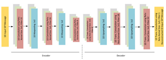
Figure 3. D1-DCAE Model: The encoder part consists of three blocks of convolutional layers and max-pooling layers. The decoder part consists of three blocks of transpose-convolutional layers and upsampling layers. At the end is a convolution layer with one feature map and a flattened layer.

In Equation (4), $H^0$ represents the input X, ∗ donates the convolution operation, f is the RelU activation function, $DownSampling$ is the max-pooling function, and L is the number of blocks of the encoder. As a result, the encoder outputs $H^L$, which represents the lower-dimensional latent representation H.

The decoder is a mirrored version of the encoder, aiming to reconstruct the input from H. Each decoder block features a deconvolutional layer with a 1 × 3 kernel and a stride of 1, followed by an upsampling layer with a 1 × 2 filter and a stride of 2, resulting in a doubling of the number and dimensions of feature maps after each block. Thus, the decoder outputs $X^{\prime }$, which has the same dimensions as the input X. The decoder learns how to output $X^{\prime }$, a reconstructed version of the input X, given the lower dimensional latent representation H. That can be formulated as follows:

$$X^{\prime l}=UpSampling\left(g\left(X^{\prime l-1}\ast W^{\prime lT}+b^{\prime l}\right)\right),l\in \{1,2,\cdots ,L\}$$

(5)

In Equation (5), $X^{\prime 0}$ represents the latent representation. H, g is the same activation function as f, $UpSampling$ is an upsampling function, and L is the number of blocks of the decoder, which is the same as the encoder. As a result, the decoder outputs $X^{\prime L}$ (i.e., $X^{\prime }$), a reconstructed version of the input X. After the decoder, a 1D convolution layer with one feature map is added, followed by a flattened layer, in order to reshape $X^{\prime }$ dimensions to be exactly like the X dimensions.

The following is the pseudocode for anomaly detection using the D1-DCAE Model:

Autoencoder Model—Encoder

Block 1

conv1 = ConvolutionalLayer (input, input_channels, 32, kernel_size = 3, stride = 1)

relu1 = ReLU (conv1)

pool1 = MaxPooling (relu1, filter_size = 2, stride = 2)

Block 2

conv2 = ConvolutionalLayer (pool1, 32, 16, kernel_size = 3, stride = 1)

relu2 = ReLU (conv2)

pool2 = MaxPooling (relu2, filter_size = 2, stride = 2)

Block 3

conv3 = ConvolutionalLayer (pool2, 16, 8, kernel_size = 3, stride = 1)

relu3 = ReLU (conv3)

Autoencoder Model—Decoder

Block 3 (Mirror of the encoder)

deconv3 = DeconvolutionalLayer (relu3, 8, 16, kernel_size = 3, stride = 1)

deconv_relu3 = ReLU (deconv3)

upsample2 = Upsampling (deconv_relu3, pool2, filter_size = 2, stride = 2)

Block 2 (Mirror of the encoder)

deconv2 = DeconvolutionalLayer (upsample2, 16, 32, kernel_size = 3, stride = 1)

deconv_relu2 = ReLU (deconv2)

upsample1 = Upsampling (deconv_relu2, pool1, filter_size = 2, stride = 2)

Block 1 (Mirror of the encoder)

deconv1 = DeconvolutionalLayer (upsample1, 32, input_channels, kernel_size = 3, stride = 1)

relu1_dec = ReLU (deconv1)

Additional layers

deconv_out = DeconvolutionalLayer(relu1_dec, 1, 1, kernel_size = 3, stride=2)

dense = DenseLayer(deconv_out, input_length, 1)

flatten = FlattenLayer(dense)

output = flatten

Anomaly Detection using Autoencoder Model

threshold = predefined_threshold_value

for each input_data in test_data:

encoded_output = encoder(input_data)

decoded_output = decoder(encoded_output)

Calculate reconstruction loss (Mean Absolute Error)

reconstruction_loss = mean_absolute_error (decoded_output,    input_data)

if reconstruction_loss > threshold:

Anomaly detected

Take appropriate action or record the anomaly

else:

Normal data

4. Datasets

VoIP suffers from a severe shortage of publicly available traffic datasets, and there is no benchmark dataset [30]. The two publicly available datasets are used to ensure the validity of the proposed model.

The INRIA dataset [16] was developed in 2010. The authors prepared a network consisting of two computers that have one hundred instances of VoIP bots used to generate the normal traffic, a server that contains SIP server software (i.e., Asterisk and Opensips), and a computer that contains the attack tools to produce the attack traffic.

This dataset contains two types of VoIP attacks: INVITE flooding and SPIT. In addition, attack messages were generated at different intensities. The most important advantage of this dataset is the utilization of different data sources: server logs stored as .txt files, CDRs stored as .csv files, and network traffic stored as .cap files. Every type of these data sources is vital for the detection of VoIP attacks; for example, the logs of the Opensips server have different probes that can be utilized for detecting unusual memory consumption and processing.

Recently, a new VoIP traffic dataset (i.e., RIT dataset) was generated to help in developing machine learning models for detecting VoIP attacks [31]. A test bed consists of four computers to generate normal traffic, an Asterisk server, and a computer to act as an attacker.

This dataset contains various attacks (i.e., REGISTER hijacking, RTP flooding, REGISTER flooding, BYE, and SPIT) with different scenarios. In addition, the authors utilized attack tools that are usually used to exploit weaknesses in VoIP networks to produce useful attack traffic data. Although this dataset has VoIP traffic from attacks larger than the INRIA dataset, it does not contain CDRs or server logs.

Below is a sample of a SPIT message from the INRIA dataset.

INVITE sip:Bot3@193.169.2.14 SIP/2.0

Via: SIP/2.0/UDP 193.169.2.15:5060;branch=z9hG4bK5287dad4

Max-Forwards: 70

From: “Your Best Friend” <sip:spitter3@SpitHostfr@193.169.2.15>;tag=as1d36c938

To: <sip:Bot3@193.169.2.14>

Contact: <sip:spitter3@SpitHostfr@193.169.2.15>

Call-ID: 08107350692bdcc34170a2ce4b2d121d@193.169.2.15

CSeq: 102 INVITE

User-Agent: Asterisk PBX 1.6.2.0 rc2-0ubuntu1.2

Date: Mon, 01 Feb 2010 16:29:59 GMT

Content-Type: application/sdp

Content-Length: 323

v = 0

o = root 183860900 183860900 193.169.2.15

s = Asterisk PBX 1.6.2.0 rc2-0ubuntu1.2

c = IN IP4 193.169.2.15

t = 0 0

m = audio 13352 RTP/AVP 3 0 8 101

a = rtpmap:3 GSM/8000

a = rtpmap:0 PCMU/8000

a = rtpmap:8 PCMA/8000

a = fmtp:101 0-16

a = silenceSupp:off

a = ptime:20

a = sendrecv

Below is an INVITE message from the RIT dataset.

INVITE sip:7000@10.10.10.22 SIP/2.0

Via: SIP/2.0/UDP 194.170.1.127:5060;branch=z9hG4bK12aeded1

Max-Forwards: 70

From: “from-extensions” <sip:6000@194.170.1.127>;tag=as4b0f6d9c

To: <sip:7000@10.10.10.22;transport=udp>

Contact: <sip:6000@194.170.1.127:5060>

Call-ID: 68462c94209b99490e38fc8062ec1521@194.170.1.127:5060

CSeq: 102 INVITE

Date: Wed, 19 Aug 2020 09:44:18 GMT

Content-Type: application/sdp

Content-Length: 311

v = 0

o = root 245855357 245855357 194.170.1.127

s = Asterisk PBX 16.12.0

c = IN IP4 194.170.1.127

t = 0 0

m = audio 10942 RTP/AVP 0 8 9 3 101

a = rtpmap:0 PCMU/8000

a = rtpmap:8 PCMA/8000

a = rtpmap:9 G722/8000

a = rtpmap:3 GSM/8000

a = rtpmap:101 telephone-event/8000

a = fmtp:101 0-16

a = maxptime:150

a = sendrecv

The INRIA dataset consists of 63,584 messages, with 3584 of them being SPIT messages and the remaining messages considered normal. On the other hand, the RIT dataset comprises 64,000 messages, with 4000 of them classified as SPIT. In order to allocate the available SPIT messages for validation and testing purposes, an equal division was employed.

The RIT dataset, which is a recent publication, has not yet been utilized as a benchmark for VoIP classification systems. In contrast, the INRIA dataset, published in 2010, has been extensively employed in the detection of VoIP attacks [15,24,32].

5. Experiments

In this section, the experiments on fine-tuning the D1-DCAE model parameters over the aforementioned datasets are addressed to achieve the best performance. In addition, the performance of the D1-DCAE model is compared with several classical anomaly detection approaches.

5.1. Setup

All the experiments were conducted on the Google Colab platform. The experiments for the D1-DCAE model were executed using a Tesla T4 GPU with 12 GB of memory. In addition, Keras and TensorFlow [33] libraries were used for the implementation. For the classical machine learning anomaly detection algorithms experiments, an AMD EPYC 7B12 CPU with 24 GB of memory and the Scikit-learn [34] library were used for implementing their models.

Furthermore, each dataset was split into 3 sections, 80% for training, 10% for fine-tuning model parameters (i.e., validation dataset), and 10% (i.e., unseen dataset) for testing the model and reporting detection performance results.

5.2. Training of D1-DCAE Model

The optimization of the trainable parameters in deep neural networks heavily relies on the training process, which directly impacts their performance. Hence, to achieve the highest possible performance of the 1D-DCAE model, the training process was conducted with extreme care. The main aim was to ensure the model’s high reconstruction capacity and discriminative ability. In addition, various experiments were implemented using different training hyperparameters. In order to minimize the loss (i.e., reconstruction loss), the training process was designed such that it utilized the minibatch gradient descent optimization approach and employed the Adam update rule [35] considering its fast convergence rate and lower memory requirements. Finally, a batch of 32 training samples (i.e., minibatch) and a learning rate of 0.001 are utilized.

The loss computed over the minibatch is used in backpropagation to balance the trade-off between the model’s robustness and efficiency. The MAE is considered a reconstruction loss because it results in the best performance. Notably, the Xavier method [36] is used to initialize all of the model’s trainable parameters in order to keep the backpropagated gradients and activation values within a tolerable range. The 1D-DCAE model is trained using normal SIP messages solely after applying the feature extraction steps explained in Section 3.2. As every batch of normal SIP messages in the training dataset flows through the model’s deep network during each iteration (i.e., epoch) of the training process, the model’s trainable parameters are updated in such a way as to minimize the reconstruction loss. After many epochs (typically more than 150 epochs), the reconstruction loss reaches its minimum, and the encoder part learns how to encode the relevant features of a normal SIP message into a lower dimensional latent representation H with a 50 times decrease in dimension. Furthermore, the decoder part of the model also learns how to reconstruct a normal SIP message from its encoded features in the latent representation H.

5.3. Performance Metrics

The D1-DCAE model was tested and reported on its detection performance in terms of F1 score, accuracy, precision, recall, Area Under the ROC Curve (AUC), and False Positive Rate (FPR).

The most important metrics that are utilized to evaluate the 1D-DCAE model are F1 score and AUC [37]. The F1 score is made up of precision and recall values.

$$\mathrm{Precision}=\frac{\mathrm{True}\mathrm{Positive}}{\mathrm{True}\mathrm{Positive}+\mathrm{False}\mathrm{Positive}}$$

(6)

$$\mathrm{Recall}=\frac{\mathrm{True}\mathrm{Positive}}{\mathrm{True}\mathrm{Positive}+\mathrm{False}\mathrm{Negative}}$$

(7)

$$\mathrm{F}1=2\ast \frac{\mathrm{Precision}\ast \mathrm{Recall}}{\mathrm{Precision}+\mathrm{Recall}}$$

(8)

Precision, computed in Equation (6), measures the proportion of true positive cases identified out of all predicted positive cases, and recall, computed in Equation (7), measures the proportion of true positive cases identified out of all actual positive cases. The F1 score is calculated in Equation (8) based on these two metrics and is considered a more accurate measure of model evaluation.

When evaluating the performance of an ML model, the F1 score and accuracy are often compared. In this work, the F1 score was chosen over accuracy for two reasons [38]. First, the accuracy score is influenced by the rate of true negatives, which may not be significant in real-life scenarios. In contrast, the F1 score is only affected by true positives, false positives, and false negatives, making it a more appropriate metric for the proposed model, which focuses on classifying intrusion attempts as positive. Second, the F1 score is more appropriate for datasets with imbalanced distributions of positive and negative cases. For imbalanced datasets, accuracy may be biased towards more frequent classes, resulting in lower classification accuracy for less frequent classes. This is particularly important for positive instances, which represent attacks or intrusion attempts and are often a minority class in intrusion detection datasets.

In addition to the F1 score, the Receiver Operating Characteristics (ROCs) metric is a widely accepted metric for assessing the performance of ML models [37]. ROC is used to evaluate the relationship between recall (i.e., sensitivity) and precision (i.e., specificity) for different threshold values in classification. The Area Under the Curve (AUC) is a measure of the ROC evaluation. A higher AUC value indicates better model performance.

5.4. Reconstruction Error Threshold

As explained in Section 3.1, the distribution of the reconstruction error of SPIT messages has a mean value larger than the reconstruction error distribution mean value of normal SIP messages. Therefore, a threshold value should be chosen, above which an SIP message is considered a SPIT message.

For the D1-DCAE model, the values from 6 to 28 are tested for the reconstruction error threshold. Figure 4 and Figure 5 show the reconstruction error threshold against the model detection performance for the INRIA and RIT validation datasets. In the case of the INRIA dataset, the best F1 score and AUC were achieved when the reconstruction error threshold equals 16, while the best F1 score and AUC for the RIT dataset were achieved at a value of 20.

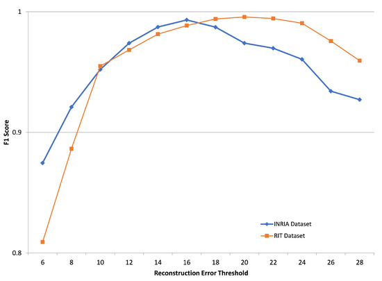
Figure 4. F1 score of the D1-DCAE model over INRIA and RIT datasets for several reconstruction error thresholds.

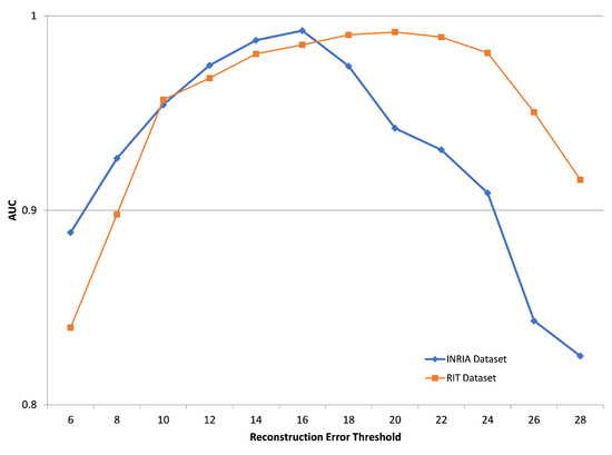
Figure 5. AUC of the D1-DCAE model over INRIA and RIT datasets for several reconstruction error thresholds.

5.5. Results and Discussion

The experiments commenced by fine-tuning the hyperparameters of the D1-DCAE model that were mentioned in Section 5.2, in addition to adjusting the reconstruction error threshold that was explained in Section 3.2 to achieve a high F1 score. As shown in Table 1, the D1-DCAE model achieved 99.32% and 99.56% F1 scores over the INRIA and RIT datasets, respectively. In addition, the number of misclassified messages was very low, as shown in Figure 6

Table 1. Performance of the D1-DCAE model over the INRIA and RIT datasets.

Dataset	F1 Score	AUC
INRIA	99.32%	99.25%
RIT	99.56%	99.18%

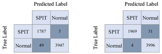
Figure 6. Confusion matrix of the D1-DCAE model over the INRIA and RIT datasets.

To compare the D1-DCAE model with classical anomaly detection approaches, the most common models [8], namely, isolation forest [39], OC-SVM [6], KDE [7], and Gaussian Mixture Model (GMM) [40] were chosen. Furthermore, the parameters of these models were fine-tuned to achieve their best performance for the validation dataset.

The results of the aforementioned models over the INRIA dataset are shown in Table 2. The D1-DCAE model achieved the best accuracy, F1 score, and AUC. Furthermore, FPR was 1.23%.

Table 2. Comparing performances of the D1-DCAE model and the classical anomaly detection models over the INRIA dataset.

Approach	Accuracy	F1 Score	Precision	Recall	AUC	FPR
D1-DCAE	99.07%	99.32%	99.87%	98.77%	99.25%	1.226
GMM [40]	81.29%	87.43%	81.53%	94.24%	73.32%	5.756
OC-SVM [6]	85.66%	90.52%	83.26%	99.17%	80.12%	0.862
KDE [7]	86.78%	91.05%	85.51%	97.35%	80.29%	2.653
Isolation Forest [39]	82.05%	87.39%	84.86%	90.07%	86.58%	9.935
Note: The highest value in each metric is in bold.

Testing the same models over the RIT dataset achieved better performance than the INRIA dataset as shown in Table 3. The D1-DCAE model achieved the best accuracy and F1 score with only 0.1% FPR.

Table 3. Comparing performances of the D1-DCAE model and the classical anomaly detection models over the RIT dataset.

Approach	Accuracy	F1 Score	Precision	Recall	AUC	FPR
D1-DCAE	99.42%	99.56%	99.23%	99.90%	99.18%	0.1
GMM [40]	90.08%	93.08%	87.05%	100.00%	85.13%	0.0
OC-SVM [6]	97.90%	98.44%	97.71%	99.18%	99.49%	0.825
KDE [7]	91.12%	93.75%	88.24%	100.00%	88.24%	0.0
Isolation Forest [39]	98.00%	98.48%	99.97%	97.03%	99.72%	2.975
Note: The highest value in each metric is in bold.

6. Conclusions

In this paper, a novel anomaly detection model, D1-DCAE, based on a deep one-class denoising convolutional autoencoder, is introduced. This model is intended to learn the underlying normal pattern of data and detect anomalies from the learned pattern. Using two publicly available datasets, INRIA and RIT, the performance of the D1-DCAE model is compared to that of the classical anomaly detection approaches. The proposed D1-DCAE outperforms the classical models in terms of accuracy, F1 score, and AUC. The experimental results have also shown that D1-DCAE achieved a lower false positive rate than the traditional methods. These outcomes indicate that the proposed model can be an effective and efficient solution for anomaly detection tasks in various domains. It is worth noting that one limitation of autoencoders is the potential impact of noise and the presence of anomalies in the training data on the extraction of relevant feature representations. To address this issue, robust deep autoencoders can be employed. Future research directions may involve reducing the number of network traffic features selected to enhance the model’s complexity and accuracy. Additionally, the implementation of a fine-grained model could be explored to investigate various VoIP attacks in greater detail.

References

- Jacobson, V.; Frederick, R.; Casner, S.; Schulzrinne, H. RTP: A Transport Protocol for Real-Time Applications. IETF RFC 3550. 2003. Available online: https://www.researchgate.net/publication/246511581_RTP_A_Transport_Protocol_for_Real-time_Applications (accessed on 1 June 2023).
- Rosenberg, J. SIP: Session Initiation Protocol. IETF RFC 3261. 2002. Available online: https://www.researchgate.net/publication/2811784_SIP_Session_Initiation_Protocol (accessed on 1 June 2023).
- Inc, C. Cisco Annual Internet Report (2018–2023) White Paper. 2020. Available online: http://shorturl.at/ehou4 (accessed on 1 January 2023).
- Javed, I.T.; Toumi, K.; Alharbi, F.; Margaria, T.; Crespi, N. Detecting nuisance calls over internet telephony using caller reputation. Electronics 2021, 10, 353. [Google Scholar] [CrossRef]
- Azad, M.A.; Morla, R.; Salah, K. Systems and methods for SPIT detection in VoIP: Survey and future directions. Comput. Secur. 2018, 77, 1–20. [Google Scholar] [CrossRef]
- Schölkopf, B.; Platt, J.C.; Shawe-Taylor, J.; Smola, A.J.; Williamson, R.C. Estimating the support of a high-dimensional distribution. Neural Comput. 2001, 13, 1443–1471. [Google Scholar] [CrossRef] [PubMed]
- Cao, V.L.; Nicolau, M.; McDermott, J. One-class classification for anomaly detection with kernel density estimation and genetic programming. In Proceedings of the European Conference on Genetic Programming, Porto, Portugal, 30 March–1 April 2016; Springer: Cham, Switzerland, 2016; pp. 3–18. [Google Scholar]
- Ruff, L.; Kauffmann, J.R.; Vandermeulen, R.A.; Montavon, G.; Samek, W.; Kloft, M.; Dietterich, T.G.; Müller, K.R. A unifying review of deep and shallow anomaly detection. Proc. IEEE 2021, 109, 756–795. [Google Scholar] [CrossRef]
- Kramer, M.A. Nonlinear principal component analysis using autoassociative neural networks. AIChE J. 1991, 7, 233–243. [Google Scholar] [CrossRef]
- Tian, Y.; Mirzabagheri, M.; Tirandazi, P.; Bamakan, S.M.H. A non-convex semi-supervised approach to opinion spam detection by ramp-one class SVM. Inf. Process. Manag. 2020, 57, 102381. [Google Scholar] [CrossRef]
- Tama, B.A.; Comuzzi, M.; Rhee, K.H. TSE-IDS: A two-stage classifier ensemble for intelligent anomaly-based intrusion detection system. IEEE Access 2019, 7, 94497–94507. [Google Scholar] [CrossRef]
- Azrour, M.; Farhaoui, Y.; Ouanan, M.; Guezzaz, A. SPIT detection in telephony over IP using K-means algorithm. Procedia Comput. Sci. 2019, 148, 542–551. [Google Scholar] [CrossRef]
- Swarnkar, M.; Hubballi, N. SpamDetector: Detecting spam callers in Voice over Internet Protocol with graph anomalies. Secur. Priv. 2019, 2, e54. [Google Scholar] [CrossRef]
- Azad, M.A.; Alazab, M.; Riaz, F.; Arshad, J.; Abullah, T. Socioscope: I know who you are, a robo, human caller or service number. Future Gener. Comput. Syst. 2020, 105, 297–307. [Google Scholar] [CrossRef]
- Pereira, D.; Oliveira, R. Detection of Signaling Vulnerabilities in Session Initiation Protocol. In Proceedings of the Doctoral Conference on Computing, Electrical and Industrial Systems, Costa de Caparica, Portugal, 7–9 July 2019; Springer: Cham, Switzerland, 2021; pp. 209–217. [Google Scholar]
- Nassar, M.; State, R.; Festor, O. Labeled VoIP data-set for intrusion detection evaluation. In Proceedings of the Meeting of the European Network of Universities and Companies in Information and Communication Engineering, Trondheim, Norway, 28–30 June 2010; Springer: Cham, Switzerland, 2010; pp. 97–106. [Google Scholar]
- Pereira, D.; Oliveira, R. Detection of Abnormal SIP Signaling Patterns: A Deep Learning Comparison. Computers 2022, 11, 27. [Google Scholar] [CrossRef]
- LeCun, Y.; Kavukcuoglu, K.; Farabet, C. Convolutional networks and applications in vision. In Proceedings of the 2010 IEEE International Symposium on Circuits and Systems, IEEE, Paris, France, 30 May–2 June 2010; pp. 253–256. [Google Scholar]
- Nazih, W.; Hifny, Y.; Elkilani, W.S.; Dhahri, H.; Abdelkader, T. Countering ddos attacks in sip based voip networks using recurrent neural networks. Sensors 2020, 20, 5875. [Google Scholar] [CrossRef] [PubMed]
- Tas, I.M.; Baktir, S. A Novel Approach for Efficient Mitigation against the SIP-Based DRDoS Attack. Appl. Sci. 2023, 13, 1864. [Google Scholar] [CrossRef]
- Henry, A.; Gautam, S.; Khanna, S.; Rabie, K.; Shongwe, T.; Bhattacharya, P.; Sharma, B.; Chowdhury, S. Composition of Hybrid Deep Learning Model and Feature Optimization for Intrusion Detection System. Sensors 2023, 23, 890. [Google Scholar] [CrossRef]
- Kasongo, S.M. A deep learning technique for intrusion detection system using a Recurrent Neural Networks based framework. Comput. Commun. 2023, 199, 113–125. [Google Scholar] [CrossRef]
- Chaganti, R.; Suliman, W.; Ravi, V.; Dua, A. Deep Learning Approach for SDN-Enabled Intrusion Detection System in IoT Networks. Information 2023, 14, 41. [Google Scholar] [CrossRef]
- Nazih, W.; Hifny, Y.; Elkilani, W.; Abdelkader, T.; Faheem, H. Efficient Detection of Attacks in SIP Based VoIP Networks using Linear l1-SVM Classifier. Int. J. Comput. Commun. Control. 2019, 14, 518–529. [Google Scholar] [CrossRef]
- Mikolov, T.; Yih, W.t.; Zweig, G. Linguistic regularities in continuous space word representations. In Proceedings of the 2013 Conference of the North American Chapter of the Association for Computational Linguistics: Human Language Technologies, Atlanta, GA, USA, 9–14 June 2013; pp. 746–751. [Google Scholar]
- Japkowicz, N.; Myers, C.; Gluck, M. A novelty detection approach to classification. In Proceedings of the 14th International Joint Conference on Artificial Intelligence, Montreal, QC, Canada, 20–25 August 1995; Volume 1, pp. 518–523. [Google Scholar]
- Hawkins, S.; He, H.; Williams, G.; Baxter, R. Outlier detection using replicator neural networks. In Proceedings of the International Conference on Data Warehousing and Knowledge Discovery, Aix-en-Provence, France, 4–6 September 2002; Springer: Berlin/Heidelberg, Germany, 2002; pp. 170–180. [Google Scholar]
- Masci, J.; Meier, U.; Cireşan, D.; Schmidhuber, J. Stacked convolutional auto-encoders for hierarchical feature extraction. In Proceedings of the International Conference on Artificial Neural Networks, Espoo, Finland, 14–17 June 2011; Springer: Berlin/Heidelberg, Germany, 2011; pp. 52–59. [Google Scholar]
- Nair, V.; Hinton, G.E. Rectified linear units improve restricted boltzmann machines. In Proceedings of the 27th International Conference on Machine Learning (ICML-10), Haifa, Israel, 21–24 June 2010. [Google Scholar]
- Nazih, W.; Elkilani, W.S.; Dhahri, H.; Abdelkader, T. Survey of countering DoS/DDoS attacks on SIP based VoIP networks. Electronics 2020, 9, 1827. [Google Scholar] [CrossRef]
- Alvares, C.; Dinesh, D.; Alvi, S.; Gautam, T.; Hasib, M.; Raza, A. Dataset of attacks on a live enterprise VoIP network for machine learning based intrusion detection and prevention systems. Comput. Netw. 2021, 197, 108283. [Google Scholar] [CrossRef]
- Umer, M.F.; Sher, M.; Bi, Y. A two-stage flow-based intrusion detection model for next-generation networks. PLoS ONE 2018, 13, e0180945. [Google Scholar] [CrossRef] [PubMed]
- Abadi, M.; Barham, P.; Chen, J.; Chen, Z.; Davis, A.; Dean, J.; Devin, M.; Ghemawat, S.; Irving, G.; Isard, M.; et al. Tensorflow: A system for large-scale machine learning. In Proceedings of the 12th {USENIX} Symposium on Operating Systems Design and Implementation ({OSDI} 16), Savannah, GA, USA, 2–4 November 2016; pp. 265–283. [Google Scholar]
- Pedregosa, F.; Varoquaux, G.; Gramfort, A.; Michel, V.; Thirion, B.; Grisel, O.; Blondel, M.; Prettenhofer, P.; Weiss, R.; Dubourg, V.; et al. Scikit-learn: Machine learning in Python. J. Mach. Learn. Res. 2011, 12, 2825–2830. [Google Scholar]
- Kingma, D.P.; Ba, J. Adam: A method for stochastic optimization. arXiv 2014, arXiv:1412.6980. [Google Scholar]
- Glorot, X.; Bengio, Y. Understanding the difficulty of training deep feedforward neural networks. In Proceedings of the Thirteenth International Conference on Artificial Intelligence and Statistics, JMLR Workshop and Conference Proceedings, Sardinia, Italy, 13–15 May 2010; pp. 249–256. [Google Scholar]
- Tufan, E.; Tezcan, C.; Acartürk, C. Anomaly-based intrusion detection by machine learning: A case study on probing attacks to an institutional network. IEEE Access 2021, 9, 50078–50092. [Google Scholar] [CrossRef]
- Weiss, G.; He, H.; Ma, Y. Foundations of Imbalanced Learning. Imbalanced Learning: Foundations, Algorithms, and Applications; John Wiley & Sons: Hoboken, NJ, USA, 2013. [Google Scholar]
- Liu, F.T.; Ting, K.M.; Zhou, Z.H. Isolation-based anomaly detection. ACM Trans. Knowl. Discov. Data (TKDD) 2012, 6, 1–39. [Google Scholar] [CrossRef]
- Kemmler, M.; Rodner, E.; Wacker, E.S.; Denzler, J. One-class classification with Gaussian processes. Pattern Recognit. 2013, 46, 3507–3518. [Google Scholar] [CrossRef]
Disclaimer/Publisher’s Note: The statements, opinions and data contained in all publications are solely those of the individual author(s) and contributor(s) and not of MDPI and/or the editor(s). MDPI and/or the editor(s) disclaim responsibility for any injury to people or property resulting from any ideas, methods, instructions or products referred to in the content. |
© 2023 by the authors. Licensee MDPI, Basel, Switzerland. This article is an open access article distributed under the terms and conditions of the Creative Commons Attribution (CC BY) license (https://creativecommons.org/licenses/by/4.0/).