Abstract
A render is the first protective layer of exterior walls against the outdoor climate, which, due to its constitution, aims to gradually slow down the liquid moisture penetration to prevent it from reaching the wall inner layers. Due to the future expected changes in the outdoor climate, today’s exterior mortar might not be adequately designed to protect these walls. This paper aims to analyse the influence of mortars on the hygrothermal performance of solid brick walls under current and future climates. The study includes four types of assemblies and three types of mortars, and it was carried out for Lisbon and three other climates by using a computational simulation tool. Finally, the moisture gains and respective reach due to the future wind-driven rain (WDR) spells were assessed by means of using future weather files for Lisbon’s climate. It was shown that the solid brick layer is influenced differently depending on the characteristics of the mortar layers and outdoor conditions. In terms of WDR spells, aside from the precipitation and the spell period, the distribution of the WDR events within the spell also conditions the dryness of the assembly. The depth that the outdoor moisture was able to reach varies between 94 and 200 mm.
1. Introduction
Since the end of the 20th century, there has been an increasing concern for the world’s resources, namely the energy sources and consumption rates. This is visible throughout the policies recently adopted in all sectors of industry, including the construction sector. In Europe, the residential sector is responsible for approximately 40% of the final energy consumption [1].
In buildings, the energy consumption can be drastically influenced by the hygrothermal behaviour of the exterior envelopes [2]. It is possible to relate their behaviour and a building’s energy consumption through the concept of thermal transmittance [3]. This thermal transmittance is usually calculated in steady-state conditions since it only takes into consideration the thermal point of view. However, most of the materials used in buildings may vary their water content according to the boundary conditions, which are constantly changing due to their stochastic nature [4]. This occurs because most of the materials used in buildings are porous materials [5]. Hence, they can store moisture [6], which is normally described by the concept of moisture storage function [7]. Consequently, the thermal transmittance of building elements is not constant [8]. Their variance is greatly influenced by the wall assembly configuration and respective building properties [8], namely moisture-impregnability-related concepts, such as the water absorption coefficient or the water vapour diffusion resistance factor [6].
This paper focus on the hygrothermal study of coated solid brick walls in different climates through one-dimensional simulation software, named WUFI (version 5.3) [9], which has been validated by many works over the years (e.g., [10,11]). This software has a wide range of applications such as assessing the risk of mould growth in a wall’s interior surface (e.g., [12,13]), assessing the freeze damage risk (e.g., [14]), determining the influence of each constituting layer or a specific surface treatment in the whole wall (e.g., [13,15]), calculating transient thermal transmittance (e.g., [8,16]), comparing the hygrothermal performance of a wall under different ambiences, and comparing measured data to simulated data (e.g., [17,18]).
For this purpose, three main goals were established for this paper. The first is to identify the effects that the application of mortar layers may have on the water contents. The second is to calculate transient thermal transmittances. The last is to determine if current mortar can withstand future moisture loads by means of determining the effects of the most demanding wind-driven rain (WDR) spells.
An exterior mortar layer (named render, R) is an important component of a wall, since it is its first protection against the exterior ambience (such as wind-driven rain) [19]. In Portugal, the traditional render is a combination of three layers with respective different objectives that aim to gradually slow down the liquid moisture penetration [20]. More recently, factory-prepared mortars are being used in construction due to their ease and quickness of application when compared to traditional mortars, but thermal-resistant mortars are also a recent appealing product due to their thermal performance [21]. Moreover, their protective function, irrespective of their origin, remains, i.e., slow down moisture penetration to prevent it from reaching the inner layers.
On the other hand, an interior mortar layer (named plaster, P) is usually applied for aesthetic reasons [20]. However, depending on their characteristics, these types of layers may cause significant changes in the hygrothermal behaviour of walls. Hence, it is important to study the hygrothermal changes that the application of these two layers may cause in the solid brick layer behaviour.
Since the steady-state thermal transmittance does not account for the moisture variation induced by the boundary conditions, the obtained values may be quite different from reality (e.g., [8,16,22]). Therefore, the difference between calculating the thermal transmittance in steady-state and in transient conditions was evaluated for all the simulated walls. This derives from the fact that most construction materials are porous, having the capacity to store fluids [6]. A higher value of moisture content in a porous material causes a higher value of thermal conductivity and, consequently, a higher value of the wall’s thermal transmittance [6], which means that for the same value of area and temperature difference, a higher amount of heat is transmitted through the element.
In this study, four types of walls were simulated: (1) a solid brick wall, (2) a rendered solid brick wall, (3) a plastered solid brick wall, and (4) a rendered and plastered solid brick wall. The simulations were computed for lime (L), cement-lime (LC), and cement (C) mortars. These three types of mortars were selected as an example of the various moisture transport characteristics of wall finishings and to illustrate the different behaviours they may induce on the performance of specific walls. These assemblies were simulated for the following four climates: Zurich (ZR), Essen (ES), San Francisco (SF), and Lisbon (LX).
The changes that the outdoor climate is expected to suffer in the future will differ in accordance with the location [23,24]. While a general increase in the outdoor temperature is expected, in terms of precipitation, a substantial increase is expected for northern Europe, while a substantial decrease is expected in southern Europe [23,25]. However, in Lisbon, an increase in extreme rain events associated with strong winds is also expected [26]. Hence, this behaviour is studied in this paper to see if this means that the outdoor moisture will be able to reach deeper thicknesses in the assembly. For this purpose, four future periods of time—near future and far future for RCP 4.5 and 8.5—will be assessed for Lisbon in order to identify the respective WDR spells in accordance with the methodology of EN ISO 15927-3 [27] and BS 8104 [28]. Finally, the hygric effect of the most demanding spells will be assessed using simulation software (WUFI®Pro).
2. Methodology
2.1. General Considerations
This paper aims to firstly identify the effects that the application of mortar layers may have on the water contents. Secondly, we aim to calculate transient thermal transmittances. Thirdly, we aim to determine if current mortar can withstand future moisture loads by means of determining the effects of the most demanding wind-driven rain (WDR) spells. To achieve these goals, simulation software (WUFI®Pro) will be used coupled to current and future climates to assess the hygrothermal performance of masonry walls. This software is reviewed in Section 2.2, while the tested masonry walls are described in Section 2.3, and the selected current and future climates are reviewed in Section 2.4.
2.2. WUFI Software
It is necessary to provide the following data for WUFI®Pro to perform (Figure 1): wall characteristics, physical and hygrothermal material properties, surface transport coefficients, initial conditions, and exterior and interior ambience conditions. The surface orientation and inclination are important inputs of a simulation since the solar radiation and wind-driven rain, if the element is not horizontal, are dependent on these parameters [29,30]. In terms of outputs for the selected assembly, it is possible to assess the temperature (°C), relative humidity (%), and water vapour partial pressure (hPa) for any of the selected locations within the assembly, water content for any layer (volume, kg/m3) or in terms of equivalent water content for the assembly (area, kg/m2), and the heat (W/m2) and moisture fluxes (kg/m2s) for the assembly surfaces and layer interfaces.
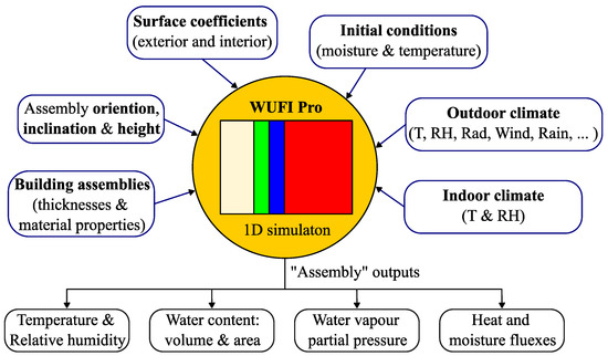
Figure 1.
Overview of the WUFI Pro inputs and respective outputs at the assembly level.
All these inputs are taken into account in WUFI’s calculation procedure. Enthalpy in a material varies according to the divergence between the heat flow through the material’s surfaces and the heat sources (condensation) or heat sinks (fusion and evaporation) in the material [6]. Condensation is the change in the physical state of matter from gas into the liquid phase. This is an exothermic phenomenon since it changes from a superior to an inferior level of molecular excitement [31]. Therefore, it releases energy, and, consequently, it increases temperature. On the other hand, evaporation is an endothermic process since the material changes from its liquid state (inferior level of molecular excitement) to its gas state (superior level of molecular excitement) [31]. Hence, it consumes energy from the system, and, consequently, it decreases temperature. Fusion is also an endothermic process because the material changes from its solid state to its liquid state [31].
In San Francisco and Lisbon, walls are not influenced by fusion, since their lowest exterior air temperature is 1.7 and 1.2 °C, respectively, and, in normal pressure conditions, water’s freezing point is near 0 °C. Hence, water never reaches the solid state, making it not possible to change from its solid to its liquid state.
The amount of moisture that exists in a wall is equal to the amount of moisture in the liquid state and gas state that is exchanged with the ambiences and the moisture sources or sinks contributions. Since moisture sources are scarce and moisture sinks related to chemical processes are low, these contributions are discarded in WUFI [6].
Since the total enthalpy, the thermal conductivity, and the heat source term are dependent on the moisture inside a building material and also due to the dependency of the liquid flux and vapour diffusion flux on the temperature, it is possible to couple the heat balance and moisture balance equations [6]. However, as it is a two-equation system, it is only solvable if there are just two variables. Taking the relations between the parameters into account, it is possible to have just two variables, i.e., temperature and relative humidity. Therefore, for one-dimensional heat and moisture transport, the following two-equation system is obtained [6]:
where ∂H/∂θ is the heat storage capacity of the moist building material (J/(m3K)), H is the total enthalpy (J/m3), θ is the temperature (°C), t is the time (s), λ is the thermal conductivity of the moist building material (W/(m·K)), hv is the evaporation heat of water (J/kg), δp is the water vapour permeability of a building material (kg/(m·s·Pa)), φ is the relative humidity (-), pv,sat is the vapour saturation pressure (Pa), ∂w/∂φ is the moisture storage capacity of the building material (kg/m3), and Dφ is the liquid conduction coefficient of the moist building material (kg/(m·s)).
WUFI is an extremally used software to assess the hygrothermal performance of assemblies in countries, for example, Norway. This user-friendly software has been validated by experimental campaigns (e.g., [32]), by comparison with other software (e.g., [33]), and against EN 15026 [34]. Finally, the software has been subjected to several updates across the years [35], which allows it to stay up-to-date in this ever-evolving scientific field.
The material properties are divided into two categories [9]. Basic properties, essential for the program, and advance properties, which can be left out. However, their omission has significant consequences for the results. The advance properties are the moisture storage function, the liquid transport coefficient for suction and for redistribution, the moisture-dependent thermal conductivity, and the moisture-dependent vapour diffusion resistance factor. The latter, in the simulated materials, is accounted for in the liquid coefficients [9].
The liquid transport coefficient of a material changes in accordance with if it is constantly supplied with water (e.g., rain event) or not. During a rain event, since a great amount of water is supplied to the material and due to their lower flow resistance, the liquid transport is governed by the larger pores [36]. On the other hand, in the absence of a water supply, the liquid transport is governed by the smaller pores due to their higher capillary pressure [36]. WUFI uses the liquid transport coefficients for suction (Dws) when water is constantly supplied to the material, and otherwise, it uses the liquid transport coefficients for redistribution (Dww); both these coefficients are highly moisture dependent. The liquid transport coefficients for each of the simulated materials are featured in Figure 3 and their water absorption coefficient in Table 1.
Surface transport coefficients describe heat and moisture exchanges between a wall surface and the ambience [37]. They differ in exterior and interior ambiences. For an exterior surface, the program considers the surface heat resistance, short-wave radiation absorptivity, long-wave radiation emissivity, and rain water absorption factor. For an interior surface, the program only considers the heat resistance.
WUFI can consider the long-wave radiation exchanges between an exterior surface and its surroundings in three different ways [9,38,39]: the heat transfer coefficient, the simplified method, and the explicit radiation balance method. However, the last two methods only run if the atmospheric counter-radiation is defined in the used climate file. Thus, in its absence, the radiation exchanges are accounted for by the heat transfer coefficient.
WUFI can calculate the heat transfer coefficient (inverse of surface heat resistance) according to the wind felt in the simulated location [40]. The water vapour transfer coefficient is automatically obtained from the heat transfer coefficient; therefore, if the wind equations are used for the heat transfer coefficient, then the water vapour transfer coefficient will vary according to the wind characteristics.
The amount of solar radiation absorbed by an exterior surface depends on its orientation and inclination and on the exterior material properties (i.e., the short-wave radiation absorptivity). Therefore, the amount of solar radiation absorbed by a façade is obtained through the following equation:
where q is the heat flux from solar radiation (W/m2), as is the short-wave radiation absorptivity (-), and I is the solar radiation vertical to the façade (W/m2).
The amount of water absorbed by a vertical surface is not equal to the quantity of rain that impacts that surface [29]. This happens because some of the impacting water splashes off [41]. WUFI takes this behaviour into consideration through the rain water absorption factor. It is normal to consider that 30% of the surface impacting water splashes off [6]. It is important to bear in mind the key influence that this solicitation has on the hygrothermal behaviour of solid brick walls [8,12]. The amount of water absorbed by a façade, which is not completely wetted, is obtained through the following equation:
where gw is the liquid flux (kg/m2s), ar is the rain water absorption factor (-), and R is the precipitation load vertical to the building component surface (-).
WUFI needs the ambience boundary conditions to be able to account for the exchanges between the wall surfaces and the respective ambience. The boundary conditions used by the program are normal rain; global and diffuse solar radiation; exterior and interior air temperatures (T); exterior and interior relative humidities (RH); barometric pressure; cloud cover; and long-wave atmospheric counter-radiation. The interior climate can be obtained using sine curves or from a standard that uses the exterior conditions for their calculation (e.g., [42]) or inputted into the model based on monitored/simulated data.
2.3. Wall Assemblies
With the purpose of identifying the alterations caused by the application of the mortar layers, all mortared assemblies were compared against a plain solid brick wall, i.e., a 220-mm solid brick wall (Figure 2a), which is considered as the standard case (SC). The study includes three types of mortared walls—exterior surface (Figure 2b), interior surface (Figure 2c), and both surfaces (Figure 2d)—and three types of mortar—lime, cement-lime, and cement. All tested mortars are 15 mm thick, and the solid brick is 220 mm thick.
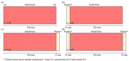
Figure 2.
Solid brick wall (a), rendered solid brick wall (b), plastered solid brick wall (c), and rendered and plastered solid brick wall (d).
In order to identify the differences between the steady-state and transient thermal transmittances, these factors were calculated for every studied wall in the four climates (Section 2.4.1). The thermal transmittance in steady-state conditions was calculated using standard thermal conductivities and the usual surface thermal resistances (i.e., 0.0588 m2K/W for the exterior ambience and 0.1250 m2K/W for the interior ambience [6]).
The thermal transmittance in transient conditions was calculated using the thermal conductivity that takes into account the moisture content of the material and the wind-dependent surface thermal resistance [8]. WUFI was used to obtain the water contents for each layer, which allows the calculation of the thermal conductivity that considers the moisture. The surface thermal resistance was calculated using WUFI’s wind-dependent equations, which depend on the wind direction and wall inclination.
The simulated materials were characterized by the Fraunhofer—Institute for Building Physics (IBP), and their characteristics can be seen in Table 1. By taking a closer look at the table, it is possible to notice that the moisture permeability decreases from lime to cement mortar. This is visible since the water absorption coefficient decreases (liquid moisture) and the water vapour diffusion resistance factor increases (vapour moisture), which means a lower drying potential [36].
All of the mortars have a much lower A-value than the solid brick, which corroborates the values obtained in the simulations (Section 3.2.1). The higher the mortar’s bulk density, the lower its thermal conductivity, which makes sense due to the fact that the thermal conductivity of the materials is related to the dimension and quantity of pores, which are inversely proportional to the bulk density [43]. Lastly, it is visible that lime has the lowest thermal conductivity among the tested mortar, and cement the highest, but this is not very significant due to this layer thickness, corresponding to a small contribution to the total thermal resistance of the tested assemblies, which varies in the range of 3.3–5.5%.

Table 1.
Properties of the materials that constitute the simulated walls. Data taken from Fraunhofer-IBP database in WUFI [9].
Table 1.
Properties of the materials that constitute the simulated walls. Data taken from Fraunhofer-IBP database in WUFI [9].
| Building Properties | Solid Brick | Mortars | ||
|---|---|---|---|---|
| Lime | Lime-Cement | Cement | ||
| Bulk density, ρ (kg/m3) | 1900.0 | 1600.0 | 1900.0 | 2000.0 |
| Porosity, ε (m3/m3) | 0.24 | 0.30 | 0.24 | 0.30 |
| Specific heat capacity-Dry, cp (J/kg·K) | 850.0 | 850.0 | 850.0 | 850.0 |
| Thermal conductivity-Dry, λ (W/m·K) | 0.60 | 0.70 | 0.80 | 1.20 |
| Water vapour diffusion resistance factor, µ (-) | 10.0 | 7.0 | 19.0 | 25.0 |
| Reference water content, w80 (kg/m3) | 18.0 | 30.0 | 45.0 | 35.0 |
| Free water saturation, wf (kg/m3) | 190.0 | 250.0 | 210.0 | 280.0 |
| Moisture-related thermal conductivity supplement, b (%/M.-%) | 15.0 | 8.0 | 8.0 | 10.0 |
| Water absorption coefficient, A (kg/m2s0.5) | 0.1100 | 0.0470 | 0.0170 | 0.0076 |
The moisture storage capacity and liquid transport coefficients for the four studied materials are presented in Figure 3. Figure 3a shows that the mortar with the highest moisture storage capacity changes throughout the relative humidity range. From 0 to 88.6% RH, it is the lime-cement, and from 88.6 to 100% RH, it is the cement mortar. It is also interesting to notice that until 75.9% RH, the lime mortar has a higher moisture storage capacity than the cement mortar and that from 93.4 to 100% RH, the lime mortar has a higher moisture storage capacity than the lime-cement mortar.
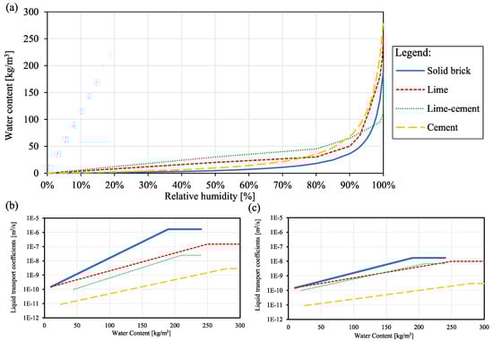
Figure 3.
Moisture storage capacity for the simulated materials (a) and liquid transport coefficients for suction (b) and redistribution (c) against water content values for the simulated materials. The maximum water content value for solid brick and lime-cement mortar is 240 kg/m3. Data taken from WUFI material database [9].
Figure 3b shows that the mortar with the highest Dws values is lime, then lime-cement, and, lastly, cement. However, the same observation cannot be made for Dww since the lime-cement mortar reaches the highest values between 137.4 and 229.6 kg/m3.
The wall’s radiation absorption behaviour differs according to the exterior layer characteristics. Since rendered and unrendered walls are simulated, two short-wave radiation absorptivity coefficients were used: 0.40 (for rendered walls) and 0.68 (for unrendered walls), which are in accordance with the literature [31,44,45,46]. The long-wave radiation exchange was determined through the simplified method for those climates.
The simulation period was chosen so that all the wall assemblies reached the dynamic equilibrium in each simulated climate. For Essen, seven years were necessary and five years for the other three climates. It is important that this level is reached because only after that will there be an equilibrium between the wall and the ambiences, and, consequently, the variation in any parameter for the following years will be the same [9]. However, it is also vital not to discard the variation in the hygrothermal parameters in the years prior to reaching the dynamic equilibrium, since it helps explain certain behaviours. Nonetheless, it is important to take into account that WUFI does not directly consider the changes over time in the hygrothermal properties of the building material.
2.4. Weather Files
2.4.1. Current Climate
This study was carried out for Lisbon, since the type of assembly is typical for this location [47]. In addition, three other climates were studied: Zurich, Essen, and San Francisco (Section 3.2). Zurich and Essen are cold climates that have moderate annual wind-driven rain (WDR), and the other two are temperate climates (San Francisco and Lisbon), not reaching below-zero temperatures, also with low and moderate annual WDR, respectively. Their relative humidity and temperature can be seen in Table 2.
Table 2.
Exterior ambience conditions for the four simulated climates in Section 3.2. Minimum, maximum, and mean values for the relative humidity and temperature.
In order to determine the effects of the exterior conditions on each wall assembly, the interior conditions were obtained through WUFI’s sine curves feature for a medium moisture load (i.e., the temperature varies between 20 and 22 °C and the relative humidity between 40 and 60%), creating equal conditions for all the simulations.
A comparison between Zurich and Lisbon is carried out in order to understand the major differences between the two types of studied climates. Lisbon has a yearly wind-driven rain sum higher than Zurich. It is important to remember that wind-driven rain depends not only on normal rain but also on the wind’s direction and velocity [41].
There is also a significant difference in terms of ambience temperature and relative humidity between the two climates. Lisbon always has the highest values of temperature, while the highest values of relative humidity change throughout the year, with Zurich presenting the highest values all year long except between the middle of February and the beginning of May. Lisbon has higher values of mean surface transfer coefficients (13.65 W/(m2 K) and 5.09 × 10⁻⁸ kg/m2s Pa) than Zurich (12.90 W/(m2 K) and 4.68 × 10⁻⁸ kg/m2s Pa). These observations support the notion that Lisbon has better drying conditions than Zurich.
2.4.2. Future Climate
The effect of climate change was assessed for Lisbon since an increase in extreme rain events associated with strong winds is expected [26,48]. Both scenario RCP 4.5 (mid-GHGs-emission scenario [49]) and scenario RCP 8.5 (high-GHGs-emission scenario [49]) and two future time frames: mid-21st century (henceforward named near future, NF) and end of the 21st century (henceforward named far future, FF) were taken into account. These future climate scenarios, named the Representative Concentration Pathway (RCP) coupled to their respective radiative forcing at the end of the century [50], belong to the 5th Assessment Report of the Intergovernmental Panel on Climate Change (IPCC) [51].
The weather files were obtained from Meteonorm software, which is a meteorological database that can provide weather files for most of the world’s locations for many of today’s used building simulation software or solar energy applications [52]. The future meteorological conditions are obtained from complex models that account for many of the parameters that affect the environment and how they will evolve, such as the greenhouse gases emissions and changes in land use [49], while also accounting for their variance and the mitigation measures promoted throughout the studied period [53]. This, of course, leads to different future weather conditions, which are in a way accounted for by considering different RCP scenarios.
Figure 4 shows the monthly averages and sums for Lisbon in terms of air temperature (Figure 4a) and relative humidity (Figure 4b), as well as precipitation (Figure 4c) and global radiation (Figure 4d) for the near past (NP), near future (NF), and far future (FF) for scenario RCP 4.5 and for the near future (NF) and far future (FF) for scenario RCP 8.5.
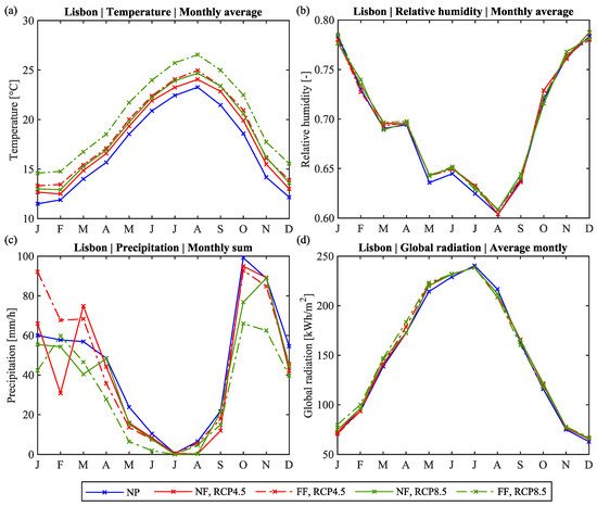
Figure 4.
Outdoor climate overview for Lisbon in the near past (NP), near future (NF), and far future (FF) for scenario RCP 4.5 and 8.5 for air temperature (a), relative humidity (b), precipitation (c), and global radiation (d).
It is visible that climate change is not responsible for significant modifications in terms of air relative humidity (Figure 4b) and global radiation (Figure 4d). The only slight variation in terms of relative humidity occurs in May, June, and July, with an average increase in relation to the near past of 0.6%. In contrast, a significant variation in the outdoor air temperature (Figure 4a) and precipitation (Figure 4c) is visible if we take climate change into account.
In terms of temperature, an overall increase is expected (Figure 4a). The highest increase is obtained by RCP 8.5 at the end of the century (FF), which is understandable since this corresponds to the more pollutant scenario [49]. RCP 8.5 at the end of the century (FF) has an average increase of 3.2 °C in relation to the near past. This is followed by RCP 4.5 at the end of the century (FF) with average increase of 1.7 °C and RCP 8.5 in the middle of the century (NF) with average increase of 1.5 °C. Finally, the lowest increase corresponds to RCP 4.5 at mid-century (NF), which has an average increase of 1.0 °C.
In relation to precipitation, the differences are more pronounced in the rainy season, whilst in the warm period of the year, the differences are obviously less significant due to the fact there is much less precipitation in this period. An increase is visible for both time periods of scenario RCP 4.5 in the first three months of the year except for February for the near future (NF). For the remainder of the year, the RCP 4.5 values are similar to the near past (NP). On the other hand, the RCP 8.5 periods have lower values than the near past, more significantly for NF at the beginning of the year and for FF at the end of the year. This evidently leads to lower annual precipitations, i.e., 453 and 378 L/(m2h).
2.4.3. Changes in the Climate of Lisbon
The changes suffered by the environment over these past years have been greatly caused by the emission of greenhouse gases due to anthropogenic activities [54]. For example, in Lisbon, which is a coastal city and the largest city in Portugal with over 2.8 M people [55], it is expected that the annual precipitation will decrease. On the other hand, it is also expected that the number of extreme phenomena with extreme rains will increase, droughts will become more frequent and more severe, and both the air temperature and the average sea level will rise [26].
In order to study the changes in the outdoor climate over the years in Lisbon, three sets of temperature and precipitation were analysed: (1) 1951–1980, (2) 1970–2000, and (3) 2005–2015. The first set was supplied by the old Meteorological Institute (now IPMA) and used by Henriques [56] to analyse the variability of the outdoor climate in eight climate representative cities of Portugal—Bragança, Porto, Portalegre, Lisboa, Beja, Faro, Ponta Delgada (Açores archipelago), and Funchal (Madeira archipelago). The second set was obtained from the IPMA website [57], and the third set was supplied by IPMA for other projects [58]. Although the third set does not cover the required 25–30 years to assess the climate variability [59], only including 11 years’ worth of data, the obtained results are still used here because they are representative of the more recent climate of Lisbon.
Overall, the mean temperature in Lisbon considerably increased from 1951–1980 to 1970–2000, with the difference amounting to +4.0 °C (Figure 5). The only month in which the average temperature corresponding to 1970–2000 is not higher than the average temperature of 1951–1980 was May (−0.3 °C). The highest increases occurred in March (+0.8 °C) and in December (+0.7 °C). The same observation can be made whilst comparing the values that correspond to 1951–1980 and 2005–2015, i.e., the mean temperature considerably increased throughout the whole year (Figure 5). The difference amounts to +7.7 °C, and the highest increases occurred in April (+1.1 °C) and in December (+1.0 °C).
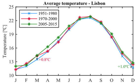
Figure 5.
Normals of the average outdoor temperature for three periods: 1951–1980 (used in Ref. [56]), 1970–2000 [57], and 2005–2015 (used in Ref. [58]).
The precipitation accumulated difference between 1951–1980 and 1970–2000 is approximately −52 L/(m2h), which means that the precipitation in Lisbon has decreased significantly from 1951–1980 to 1970–2000 (around 7%). The highest difference occurred in March, with a decrease of ca. −50 L/(m2h) (Figure 6). However, the difference in January (−25 L/(m2h)), February (−18 L/(m2h)), and December (−15 L/(m2h)) is also considerable. On the other hand, the precipitation increased substantially in May (+12 L/(m2h)) and April (+11 L/(m2h)), but it was not enough to compensate for the decrease that occurred in the other months.
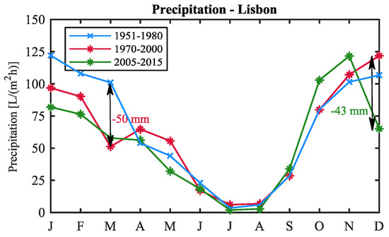
Figure 6.
Precipitation normals for three periods: 1951–1980 (used in Ref. [56]), 1970–2000 [57], and 2005–2015 (used in Ref. [58]).
When comparing 1951–1980 and 2005–2015, the difference in terms of precipitation is even higher (Figure 6), i.e., the precipitation decreased ca. −127 mm, around 16% when compared to the 1951–1980 value. The most significant decreases occurred in March (−43 mm), December (−42 L/(m2h)), and January (−40 L/(m2h)). On the other hand, the precipitation increased substantially in October (+23 L/(m2h)) and November (+20 L/(m2h)) and slightly in September (+5 L/(m2h)), but, once again, these increases are not enough to compensate for the decreases in precipitation that occur in the other months of the year.
In addition, the average monthly maximum and minimum were compared for the periods of 1951–1980 and 1970–2000. It is visible that the difference in the maximum temperatures is not as substantial as one would expect (Figure 7a). The temperature accumulated difference amounts to +1.2 °C, with the largest differences being reached in March (+0.9 °C), December, and February (+0.5 °C). On the other hand, the difference between both periods is much more significant for the minimum temperatures, with the 1970–2000 period always corresponding to higher temperatures, except for January (Figure 7b). Its accumulated difference amounts to +6.9 °C, with the largest differences being reached in July and December (+0.9 °C), closely followed by August and September (+0.8 °C).
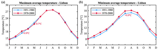
Figure 7.
Normals of the maximum (a) and minimum (b) outdoor temperatures for two periods: 1951–1980 (used in Ref. [56]) and 1970–2000 [57].
3. Results and Discussion
3.1. General Considerations
This section is divided into two main subsections: Section 3.2, in which the selected four assemblies are assessed in terms of water content (Section 3.2.1) and transient U-value (Section 3.2.2) for four current selected climates—i.e., Zurich, Essen, San Francisco, and Lisbon; and Section 3.3, in which the moisture penetration is assessed by firstly determining the critical spells (Section 3.3.1) and then by assessing the moisture content variation within the assembly during the critical spells for Lisbon whilst taking into account near-past (Section 3.3.2) and future conditions (Section 3.3.3 for RCP 4.5 and Section 3.3.4 for RCP 8.5).
Figures 14–18 were produced based on the dynamic relative humidity values for specific locations obtained from WUFI®Pro and transformed into water content values using the respective moisture storage function through a MATLAB code developed by the authors. Some of the analysed spells have an extra 24 h in addition to the end of the spell. This occurs in the cases when there is a significant wind-driven rain (WDR) event near the end of the spell, and, therefore, it is interesting to assess the drying of the assembly. This appears as a green line in the figures and is named “Dry end”.
3.2. Assemblies Hygrothermal Assessment: Current Climates
The walls are subjected to wetting and drying cycles, which are controlled by the boundary conditions and may change due to the wall configuration. In moderated water uptake walls, the wetting phase (WP, defined by the increase in water content) occurs during the rainy season, and the drying phase (DP, defined by the decrease in water content) occurs during the dry season. These cycles were defined for each of the four studied climates according to the variation in the water content of the standard case for each climate (Table 3).
Table 3.
Wetting and drying cycle for the studied climates. Each month is divided into three points: beginning, middle, and end. The wetting phase is identified in blue and the drying phase in red.
3.2.1. Water Content within Assemblies
In temperate climates, the application of a render causes a significant decrease in water content during the wetting phase and slightly higher values for the drying phase (Figure 8a,b). The decrease in water content during the wetting phase, i.e., when the wall is subjected to a great amount of moisture from the exterior ambience, is due to the fact that the renders’ moisture transport properties are lower than those of the solid brick; hence, the layer of solid brick has a lower amount of moisture. During the drying phase, i.e., when the boundary conditions compel the wall to expel moisture, the application of a render layer causes higher water contents since it reduces the evaporative capacity of the solid brick.
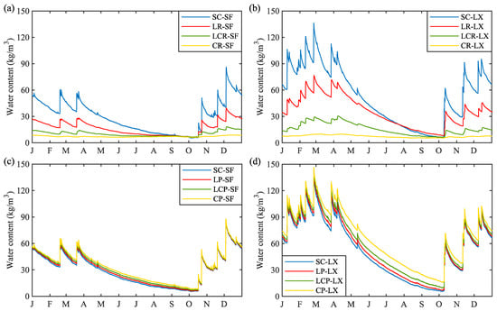
Figure 8.
Water content of the solid brick for the standard case (SC) and rendered cases in S. Francisco, SF (a), and Lisbon, LX (b) where LR is lime, LCR is lime-cement, and CR is cement renders; and water content of the solid brick layer for the standard case (SC) and plastered cases in S. Francisco, SF (c), and Lisbon, LX (d), where LP is lime, LCP is lime-cement, and CP is cement plasters.
On the other hand, the application of plaster results in an increase in water content for temperate climates, which is more obvious during the wall’s drying phase (Figure 8c,d). All unrendered simulated walls have the same layer in direct contact with the exterior ambience (i.e., solid brick). Thus, the amount of moisture that penetrates into the solid brick is similar. However, due to the mortars’ moisture transport properties, it is harder for moisture to reach the interior ambience. Consequently, moisture is stored at the interface between the solid brick and the plaster. This moisture storage could have been influenced by the moisture transport resistance, which is generated by the interface characteristics between layers. However, this type of resistance is not considered in WUFI.
These two behaviours are more significant, depending on how impermeable the mortar is to moisture. A wall coated on both surfaces has a similar behaviour to that of a rendered wall, but with slightly higher values of water content since the plaster reduces the evaporative capacity of the solid brick.
In cold climates, plasters also cause an increase in the solid brick’s water contents directly proportional to the moisture transport properties of mortars. However, the application of a render layer in this type of climate does not have all the same implications as the ones previously described for temperate climates. Although the application of a render layer also causes a decrease in water content during the wetting phase and higher water content values during the drying phase, the case with the highest water contents changes throughout the year (Figure 9).
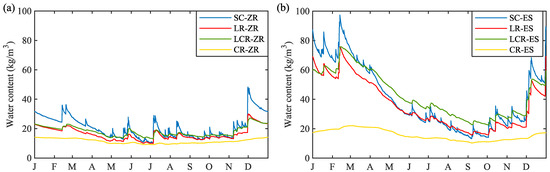
Figure 9.
Water content variation in the solid brick layer for the standard case (SC) and rendered cases in Zurich, ZR (a), and Essen, ES (b). LR—Lime, LCR—Lime-cement, and CR—cement renders.
During the wetting phase, the standard case absorbs more moisture than the other cases due to its higher moisture transport properties (see Figure 3). During the drying phase, the standard case expels moisture easier than the rendered cases, since it does not have the render layer decreasing the evaporative capacity. The lime-cement rendered case is, for most of the year, the one with the highest water contents. This is due to the wind-driven rain magnitude, which in this type of climate is almost never sufficient for the case of lime renders to surpass the lime-cement case. The cement-rendered case behaviour is quite different from the other cases due to its lower moisture transport properties. A wall coated on both surfaces has a similar behaviour to that of a rendered wall.
It is possible to understand the importance of the magnitude of wind-driven rain spells by comparing the behaviour of the rendered walls in cold and temperate climates. Therefore, the following three paragraphs only refer to the behaviour of rendered cases in two climates (Zurich and Lisbon) for the first simulation year.
Initially, the same behaviour concerning the water contents (i.e., highest values of water content correspond to the case with the most moisture-impermeable mortar—cement—and the lowest values to the case with the less moisture-impermeable mortar—lime) occurs in both climates (Figure 10 for Zurich and Figure 11b for Lisbon). However, when the wall faces a wind-driven rain spell with sufficient magnitude, the after-effect of this solicitation is different considering the type of climate.
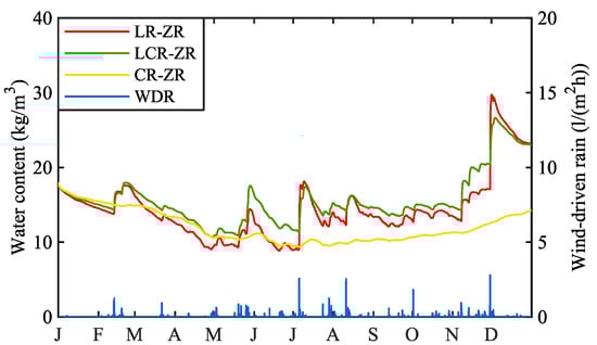
Figure 10.
Water content of the solid brick layer for the rendered cases and wind-driven rain (WDR) for the adopted conditions in Zurich (ZR) for the first simulation year. LR—Lime, LCR—Lime-cement, and CR—cement renders.
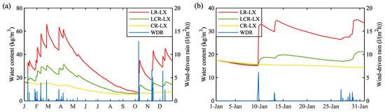
Figure 11.
Water content of the solid brick layer for the rendered cases and wind-driven rain (WDR) variation for the adopted conditions in Lisbon (LX) for the first simulation year (a) and zoom on January of the same year (b). LR—Lime, LCR—Lime-cement, and CR—cement renders.
In both climates, the less impermeable mortar (lime) attains the highest water content values. However, in Zurich, the amount of moisture absorbed by the exterior surface is not enough to compensate for the drying of the wall, and, shortly after, the lime-rendered case is surpassed by the lime-cement-rendered case (Figure 10). This does not occur in Lisbon, since the amount of moisture on the exterior surface is so substantial that it originates a very large difference between both cases, preventing the lime-cement case from surpassing the lime case (Figure 11). The cement-rendered case is a special situation, since the amount of moisture that reaches the solid brick layer is very low due to its low moisture transport properties. Furthermore, the amount of incident rain on a wall in Zurich is so low that it causes the cement-rendered case to have very different behaviour from the other two rendered cases.
The alternation of the case with the highest water content value is due to the change in the wall’s main source of moisture. When the wall was not yet subjected to the wind-driven rain spell, the main source of moisture is the interior ambience or interstitial condensation. Therefore, the more impermeable the render is to moisture, the greater the opposition for moisture to be transported across the wall will be, thus increasing the amount of moisture stored at the interface. When the wind-driven rain spell occurs, the less impermeable the render is to moisture, the higher will be the amount of moisture that penetrates into the mortar (since it offers a lower resistance to moisture transport), and, consequently, a higher value of water content is reached in the solid brick layer. The latter behaviour has a much higher magnitude than the former.
Figure 12 shows that the application of a render layer has a greater effect in temperate climates than in cold climates. For uncoated solid brick walls, Lisbon’s values are much higher than Zurich’s, namely in the wall’s wetting phase (Figure 12, in square dot). However, due to the application of the render layer, this difference decreases substantially, and in some cases, it can even cause an exchange of the climate with the highest values. This fact is quite obvious if we compare the relationship between the extreme cases for both climates, i.e., the standard case and the cement-rendered case. While for the uncoated solid brick wall in Lisbon, the water content varies between 5.5 and 136.3 kg/m3, in Zurich, it varies between 10.3 and 48.3 kg/m3, which means that the highest values are attained in Lisbon. On the other hand, for the cement-rendered cases, Zurich (varies between 9.0 and 14.2 kg/m3) attains higher values than Lisbon (varies between 5.4 and 10.1 kg/m3).
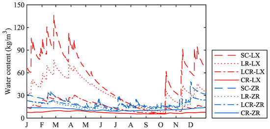
Figure 12.
Water content for the solid brick in the standard case (SC) and rendered cases for Lisbon (LX) and Zurich (ZR) in the last year of the simulation. LR—Lime, LCR—Lime-cement, and CR—cement renders.
This change is due to the lower drying conditions of the cold climates, which means that the wall is less driven to expel moisture and, consequently, has a higher water content value. As the liquid transport coefficients are highly dependent on water content (Figure 3), the moisture transport in the solid brick will be faster; therefore, the exterior surface absorbs a higher amount of moisture than in temperate climates (Table 4). The application of a render layer has a more crucial effect on temperate than on cold climates, since the decrease in water absorbed by the exterior surface is much higher in the former than in the latter climates.
Table 4.
Moisture liquid flux for the exterior surface in the standard case (SC) and rendered cases for the four studied climates. LR—Lime, LCR—Lime-cement, and CR—cement renders.
3.2.2. Assemblies Transient U-Value
A comparison between two thermal transmittances calculated for different conditions was developed for the ten types of wall assemblies in the four different climates. US is calculated in steady-state conditions and UT for transient conditions. The latter coefficient is obtained using WUFI’s outputs, and it is the average for the last year of simulation. This value directly follows the variation in the wall’s water contents.
In temperate climates, the application of a render layer causes a decrease in the difference between both thermal transmittances, which is larger the more impermeable the render is to moisture. In cold climates, the same cannot be said due to what happens with the lime-cement case. In conclusion, it can be stated that for temperate climates, the more impermeable the render is to moisture, the more real the value of thermal transmittance calculated in steady-state conditions will be (Table 5, render).
Table 5.
Thermal transmittance in steady-state (US) and in transient conditions (UT) relation in % (UT/US) for each of the tested wall assemblies in each of the four simulated climates.
The application of a plaster layer originates an increase in the differences between the thermal transmittances, which is more significant the more impermeable the plaster is to moisture (Table 5, plaster). This occurs for both types of climates and is due to the moisture storage at the interface originated by the plaster. For these cases, the relation UT/US has a minor variation but attains higher values than in the render cases (e.g., while in Essen, the UT/US for the render cases varies between 5.6 and 14.3%, that for the plaster cases varies between 16.6 and 18.5%).
The application of both layers originates identical values to the respective rendered case but with slightly higher values (Table 5, render and plaster). This happens because of the decrease in the wall’s evaporative capacity caused by the application of the plaster layer [60], resulting in higher values of water content and, consequently, higher values of thermal transmittance.
3.3. Moisture Penetration
3.3.1. WDR Spell Identification
The five periods of time selected for Lisbon, i.e., near past (NP), near future (NF), and far future (FF) for scenario RCP 4.5 and RCP 8.5, were assessed in order to identify the respective wind-driven rain (WDR) spells. For this purpose, the methodology described in EN ISO 15927-3 [27] and BS 8104 [28] was followed.
Note that the WDR spells are dependent on the orientation of the walls, so for this study, the worst-case scenario was adopted for each climate, i.e., the orientation with the highest WDR load, which is considerably dependent on the wind patterns. The selected orientation for NP was north; for RCP 4.5, in the NF, it was northeast and west for the FF, while for RCP 8.5, in the NF, it was northwest and southwest for FF. The tested assembly was the exterior lime mortared (15 mm) with brick layer (220 mm) assembly.
Figure 13 shows the number of WDR spells for each of the five selected periods as well as the respective annual precipitation. In addition to the total number of spells, four magnitudes of spells, in accordance with their respective total spell precipitation, were determined in order to identify the periods most prone to moisture penetration, i.e., total spell precipitation above 5, above 10, above 15, and above 20 L/(m2h).
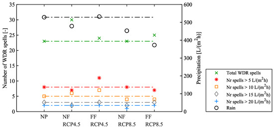
Figure 13.
Overview of the WDR spells for the five periods selected for Lisbon and the respective annual precipitation.
In general, it is visible that in the future, a greater number of WDR spells are expected (Figure 13, green cross markers), although a decrease in the precipitation is also expected for most of the studied future periods when compared with the near past (Figure 13, black circle markers). The exceptions are FF for RCP 4.5, which has slightly higher precipitation, and NF for RCP 8.5, which has the same number of total WDR spells as NP.
However, the same conclusion is not drawn for the higher total spell precipitation spells. For above 5 L/(m2h) spells, the number is very similar for the five analysed periods except for FF for RCP 4.5, which has more three spells than NP (Figure 13, red asterisk markers). For above 10 L/(m2h) spells, the RCP 4.5 periods have one to two more spells than NP, and the RCP 8.5 periods have one less spell than NP (Figure 13, orange square markers). For above 15 L/(m2h) spells, the periods in the FF for both scenarios have the same number of WDR spells as NP, but for the NF periods, they have one less spell (Figure 13, grey diamond markers). For above 20 L/(m2h) spells, the number is the same as the NP for all selected periods with the exception of NF for RCP 8.5, which has one less spell (Figure 13, blue cross markers).
The worst WDR spells, i.e., adopted as spells above 15 L/(m2h) independently of their duration, were selected for each of the five selected periods of time to assess how the selected assembly would behave in accordance with the WDR and how this would vary in accordance with climate change (Table 6). For each future scenario, two or three spells were assessed, which is not very different from the NP, but it is visible that the highest WDR spells have increased when compared with the NP. The highest WDR spell precipitation for NP is 27 L/(m2h), while for future scenarios, there is always at least one spell with a value above 30 L/(m2h), with the highest value being 33.8 L/(m2h).
Table 6.
Overview of the selected WDR spells for each of the five selected periods of time.
There is variance in the size of the spells within each scenario, but no great difference is visible if we compare the near past with any of the future scenarios; there is always a longer spell (more than 200–300 h) and a smaller spell (more than 24–100 h). In sum, an increase in the number of WDR spells is expected but not at the highest values, although an increase in the value of the spell precipitation for the highest WDR spell is observed in the future periods.
3.3.2. Near Past
Figure 14a–c presents the water content profile for the selected three spells for the near past (Table 6), while Figure 14d–f shows the respective precipitation for each of these spells. The first two spells show the results for an additional 24 h after the spells ended because they had a substantial WDR event right before the spell ended (Figure 14d,e).
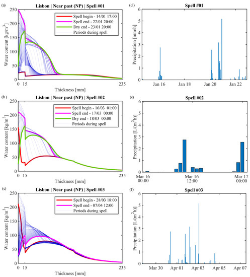
Figure 14.
Water content (kg/m3) across the wall assembly and in accordance with time for spell 1 (a), spell 2 (b), and spell 3 (c) for the near past (NP) for Lisbon and precipitation (L/(m2h)) during spell 1 (d), spell 2 (e), and spell 3 (f). The blue lines in (a–c) correspond to water content across the assembly for any given period within the corresponding spell limits.
Figure 14a corresponds to the first selected spell, which has a duration of 196 h and has a total precipitation during the spell of 27 L/(m2h). The water content reaches its highest value of 14.8 kg/m2 on 22/01 at 20:00 and its lowest value of 3.3 kg/m2 on 14/01 at 20:00. These equivalent water contents were determined as described in WUFI [9].
It is visible that when the spell starts, the water content through the assembly is rather low (i.e., 14/01 at 17:00), but, subsequently, the water content increases substantially in both materials (Figure 14a). The vertical values at the thickness of 15 mm correspond to the connection between the two materials, which have different hygric properties (Figure 3a), and, therefore, there is a discontinuity. It is also visible that once the spell starts, moisture starts to enter the assembly through the exterior layer (i.e., render) and eventually reaches the inner layer (solid brick).
For this spell, moisture can reach substantially until ca. 110 mm depth (at 17.9 kg/m3), substantially reaching the brick layer. It is also interesting to observe that when the spell ends, the moisture content in the exterior layer is rather high (Figure 14a, purple line), but 24 h later, it is already 5.3 times lower at the exterior surface. This decrease will eventually spread to the remainder of the assembly as long as there is no WDR spell soon.
Figure 14b corresponds to the second selected spell, which has a duration of 24 h and has a total precipitation during the spell of 24.2 L/(m2h). This means that for a much shorter period (i.e., 8.2 times lower), the assembly is subjected to a similar level of precipitation to the first selected spell (just 12% lower). The water content reaches its highest value of 16.0 kg/m2 on 17/03 at 00:00 and its lowest value of 6.9 kg/m2 on 16/03 at 01:00. These values mean that the amount of moisture that exists in the assembly is greater for this spell than for the first spell, i.e., a much longer spell with slightly higher precipitation.
It is visible that at the beginning of the spell (i.e., 16/03 at 01:00), the water content at the exterior surface is rather high, but it is also visible that the water content level from the interface until the middle of the solid brick layer is considerably higher than for the first spell (Figure 14a,b, red lines). This means that the masonry layer was not able to dry out the moisture that managed to penetrate the assembly due to the previous spells and, therefore, has a moisture excess. After the dry period (Figure 14b, green line), it is visible that the water content values nearer to the interface are still rather high, but they are considerably lower than when the spell ends (Figure 14b, purple line).
Nonetheless, the outdoor absorbed moisture in this spell manages to penetrate the assembly until a depth of ca. 110 mm, i.e., the same depth as the first spell, but at a much higher water content value (43.5 kg/m3) because the assembly is not able to dry out the moisture that managed to penetrate from previous spells.
Figure 14c corresponds to the third selected spell, which has a duration of 235 h and a total precipitation during the spell of 18.4 L/(m2h). In this spell, the extra period was not considered because, contrary to the other two spells, there is no significant WDR event near the end of the spell (Figure 14f). This spell has a longer period than the first spell (20% higher) but much lower total precipitation (47% lower). The water content reaches its highest value of 15.8 kg/m2 on 02/04 at 18:00 and its lowest value of 9.1 kg/m2 on 01/04 at 14:00. This shows that although this is a wider spell with lower precipitation than the second spell, it reaches similar values (Table 7), which means that the state in which the assembly is due to previous spells is also of great importance.
It is visible that at the beginning of the spell (i.e., 28/03 at 18:00), there is a great amount of moisture already trapped in the solid brick. Due to the absorbed precipitation within the spell, the values will increase throughout the assembly. Even when the spell finishes (Figure 14c, purple line), the values are still rather high, but they will decrease as the assembly dries, which is already visible at the outer layers of the exterior surface when the spell finishes. In this case, the absorbed moisture is able to reach a depth of 200 mm (at 8.9 kg/m3). By comparing this with the other spells, it is visible that the excess of moisture is increasing, since the assembly is not able to dry out all the absorbed moisture.
3.3.3. Future Climates—Scenario RCP 4.5
Near Future
Figure 15a,b present the water content profile for the tested assembly for the selected two spells for the near future for scenario 4.5 (Table 6), while Figure 15c,d show the respective precipitation for each spell. Both spells show the results for an extra 24 h after the spells have ended because they had a substantial precipitation event right before the spell ended (Figure 15c,d).
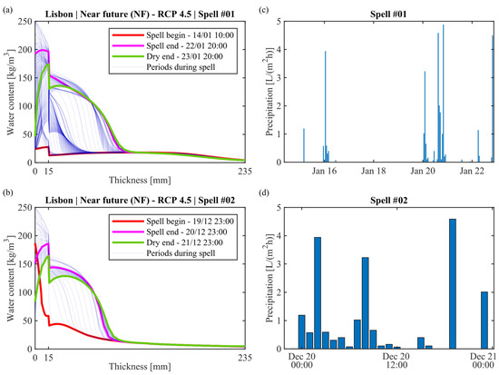
Figure 15.
Water content (kg/m3) across the wall assembly and in accordance with time for spell 1 (a) and spell 2 (b) for the near future (NF) for scenario RCP 4.5 and precipitation (L/(m2h)) during spell 1 (c) and spell 2 (d). The blue lines in (a,b) correspond to water content across the assembly for any given period within the corresponding spell limits.
Figure 15a corresponds to the first selected spell, which has a duration of 203 h and a total precipitation during the spell of 33.8 L/(m2h). The water content reaches its highest value of 15.6 kg/m2 on 22/01 at 20:00 and its lowest of 3.3 kg/m2 on 14/01 at 23:00.
The behaviour here is similar to that of the first spell in the near past (Figure 14a). The water content in the assembly starts at low values (i.e., 14/01 at 10:00), but it is visible that as time progresses, the amount of moisture within the assembly increases. The values at the exterior surface reach saturation (Figure 3) during the most significant WDR events, which eventually spread out to the remainder of the assembly (Figure 15a). By comparing the water content between the end of the spell and the extra 24 h, it is visible that the assembly manages to dry, more obviously nearer to the exterior surface for the mortar layer and closer to the interface for the solid brick (Figure 15a). Although at the interface, they may have similar RH values, they will have a considerable difference in terms of moisture content since they are different materials, and, consequently, have different moisture storage functions (Figure 3). The exterior moisture manages to penetrate up to a depth of 114 mm with 18.0 kg/m3.
Figure 15b corresponds to the second selected spell, which has a duration of 25 h and a total precipitation during the spell of 25.1 L/(m2h). Although it is a much shorter spell than the first one (88% shorter), its total precipitation is not very distant (26% shorter). The water content reaches its highest value of 14.9 kg/m2 on 20/12 at 09:00 and its lowest value of 5.5 kg/m2 on 19/12 at 23:00.
The behaviour here is similar to that of the second spell in the near past (Figure 14b), although this one occurs in December while the other occurs in March. The water content in the assembly starts at low values on the inner surface and at higher values nearest to the exterior surface (Figure 15b, red line). Nonetheless, it is visible that as time progresses, the amount of moisture within the assembly increases. The values at the exterior surface also reach saturation (Figure 3) during the most significant WDR events, which eventually spread out to the remainder of the assembly (Figure 15b). By comparing the water content between the end of the spell and the extra 24 h, it is visible that the assembly manages to dry, even more than at the beginning of the spell. This behaviour is more evident the nearer to the exterior surface we analyse (Figure 15a). The exterior moisture manages to penetrate up to 107 mm depth at 12.1 kg/m3, slightly lower than the first spell (Table 7).
In conclusion, although the second spell is a much shorter spell than the first, the amount of moisture that manages to penetrate the assembly is similar, thus reaching almost the same depth. This means that shorter spells can be as dangerous as wider ones.
Far Future
Figure 16a–c present the water content profile for the selected three spells for the far future for RCP 4.5 (Table 6), while Figure 16d–f show the respective precipitation for each spell. The three spells show the results for an extra 24 h after the spells end because they had a substantial precipitation event right before the spell ended (Figure 16d–f).
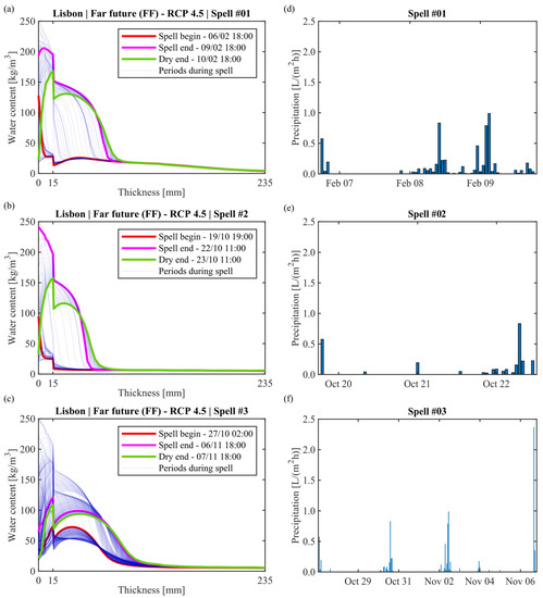
Figure 16.
Water content (kg/m3) across the wall assembly and in accordance with time for spell 1 (a), spell 2 (b), and spell 3 (c) in the far future (FF) for scenario RCP 4.5, as well as precipitation (L/(m2h)) during spell 1 (d), spell 2 (e), and spell 3 (f). The blue lines in (a–c) correspond to water content across the assembly for any given period within the corresponding spell limits.
Figure 16a shows the water content for the first selected spell, which lasts for 73 h and has a total precipitation of 16.3 L/(m2h). The highest water content value of 14.2 kg/m2 is attained on 09/02 at 17:00, while the lowest water content value of 3.5 kg/m2 is attained on 07/02 at 23:00.
At the beginning of the spell (i.e., 06/02 at 18:00), it is visible that there are rather low water content values overall, with the exception of the exterior surface (until mid-way of the mortar layer). It is visible thereafter that the water content will increase considerably through the mortar layer, followed by the section of the brick layer close to the interface zone. Once the spell ends (Figure 16a, purple lines), it is visible that the water content starts to decrease, i.e., the assembly starts to dry, more significantly near the exterior surface, but the drying effects are more visible 24 h later (Figure 16a, green lines). For this case, the outdoor moisture manages to reach a depth of 94 mm with 18.4 kg/m3.
Figure 16b shows the water content for the second selected spell, which lasts for 65 h and has a total precipitation of 22.0 L/(m2h). This spell is slightly shorter than the first (12.3% shorter), but the precipitation amounts to a higher value (35% higher). The highest water content value of 11.6 kg/m2 is attained on 22/10 at 11:00, while the lowest water content value of 1.8 kg/m2 is attained on 22/10 at 22:00. This is an interesting result that shows that it is not only the amount of precipitation or the period of spell that should be accounted for but also the distribution of the WDR events. For the first spell, the WDR events are more spread out, while in the second spell, they are more concentrated in the beginning and at the end of the spell (Figure 16d,e), which gives the wall the possibility to dry more.
It is visible that although there is a great distance between the spells, the behaviour is quite similar to the first spell, even in terms of moisture in the more inner layers (Figure 16a,b). Once the spell starts, the moisture is able to penetrate the wall, and, consequently, the moisture content increases substantially for the whole mortar layer and the solid brick’s sections nearest to the interface zone (Figure 16b). It is visible that once the spell ends (Figure 16b, purple line), the water content in the wall is still high, but 24 h later, it is already much lower (Figure 16b, green line). It is also interesting to see that although this spell has a higher total precipitation, the outdoor moisture does not reach as deep as the first spell (i.e., depth of 88 and 94 mm, respectively). This allows us to conclude that short spells with high precipitation might not be as dangerous as other spells that occur in a very humid period (Table 7).
Figure 16c shows the water content for the third selected spell, which lasts for 257 h and has a total precipitation of 31.0 L/(m2h). This means that this is the longest spell by far but also the one with the highest total precipitation, and it seems that the exterior moisture is able to reach the greatest depth of the three spells with a depth of 179 mm with 6.4 kg/m3 (Table 7). The highest water content value of 14.7 kg/m2 is attained on 02/11 at 13:00, while the lowest water content value of 5.4 kg/m2 is attained on 30/10 at 02:00.
At the beginning of the spell, the water content values are rather high when compared to the values for the other two spells, more specifically for the part of the solid brick that is near the interface zone (Figure 16c, red line). It is visible that once the spell starts, the water content across the mortar layer and solid brick zone near the interface zone also increases. However, contrary to the previous spells, there is no great difference between the end of the spell (Figure 16c, purple line) and after the extra 24 h (Figure 16c, green line). This might occur because there is a great gap between the last WDR event and the previous one (Figure 16f), and, therefore, the assembly is dryer.
In conclusion, aside from the precipitation and the spell period, the distribution of the WDR events within the spell also conditions the drying of the assembly extremely.
3.3.4. Future Climates—Scenario RCP 8.5
Near Future
Figure 17a,b present the water content profile for the selected two spells for the near future for RCP 8.5 (Table 6), while Figure 17c,d show the respective precipitation for each spell. The two spells show the results for an extra 24 h after the spells end because they had a substantial precipitation event right before their end (Figure 17c,d).
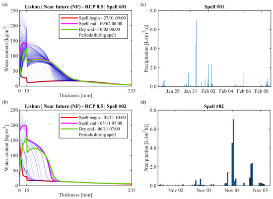
Figure 17.
Water content (kg/m3) across the wall assembly and in accordance with time for spell 1 (a) and spell 2 (b) for the near future (NF) for scenario RCP 8.5, as well as precipitation (L/(m2h)) during spell 1 (c) and spell 2 (d). The blue lines in (a,b) correspond to water content across the assembly for any given period within the corresponding spell limits.
Figure 17a shows the water content for the first selected spell, which lasts for 304 h and has a total precipitation of 33.1 L/(m2h). The highest water content value of 13.6 kg/m2 is attained on 28/01 at 06:00, while the lowest water content value of 3.0 kg/m2 is attained on 27/01 at 15:00.
It is visible that before the spell begins (i.e., 27/01 at 09:00), the water content value throughout the assembly is rather low. This means that the assembly is able to dry from the previous spells. However, as soon as the spell starts, the water content increases firstly on the exterior surface, which then spreads to the remainder of the assembly. In addition, it is also visible that the extra 24 h for drying are not enough for the brick to dry, but some substantial differences are already observed for the lime layer (Figure 17a, purple and green lines). For this case, the moisture originating from outdoors is able to reach a depth of 129 mm at 17.0 kg/m3 (Figure 17a).
Figure 17b shows the water content for the second selected spell, which lasts for 94 h and has a total precipitation of 17.2 L/(m2h). This spell is shorter than the first spell (69.1% shorter), and the precipitation is lower (48% lower). The highest water content value of 13.6 kg/m2 is attained on 05/11 at 02:00, while the lowest water content value of 3.4 kg/m2 is attained on 02/11 at 15:00. It is interesting to notice that the highest average water content is attained not right after the most significant WDR spell, i.e., 04/11, but nearly at the end of the spell.
It is visible that before the spell begins (i.e., 01/11 at 10:00), the water content value throughout the assembly is rather low with the exception of the exterior surface. Since the value is still far from the mortar maximum storage capacity (Figure 3), this means that the initial WDR spell is sufficient to increase the water content at the exterior surface. It is visible that after the spell starts, the amount of moisture within the assembly increases considerably, and there is a significant difference between the end of the spell and 24 h later, especially nearer to the exterior surface for the mortar and nearer the interface for the brick (Figure 17b, purple and green lines). For this case, the moisture originating from the outdoors is able to reach a depth of 94 mm (Figure 17a), which is not as deep as for the first spell (Table 7). This is probably because the spell is shorter as well as due to the amount of rain that impacts the wall.
Far Future
Figure 18a–c present the water content profile for the selected three spells in the far future for RCP 8.5 (Table 6), while Figure 18c–e show the respective precipitation for each spell. The last two spells show the results for an extra 24 h after the spells have ended because they had a substantial precipitation event right before the spell ended (Figure 18c,e).
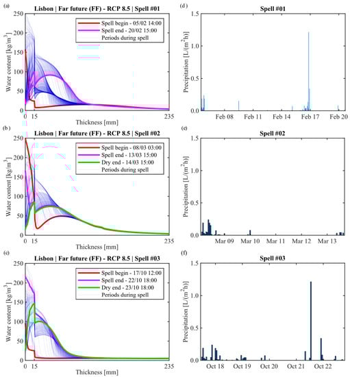
Figure 18.
Water content (kg/m3) across the wall assembly and in accordance with time for spell 1 (a), spell 2 (b), and spell 3 (c) for the far future (FF) for scenario RCP 8.5 and precipitation (L/(m2h)) during spell 1 (d), spell 2 (e), and spell 3 (f). The blue lines in (a–c) correspond to water content across the assembly for any given period within the corresponding spell limits.
Figure 18a shows the water content for the first selected spell, which lasts for 362 h and has a total precipitation of 31.0 L/(m2h). The highest water content value of 13.0 kg/m2 is attained on 16/02 at 19:00, while the lowest water content value of 3.0 kg/m2 is attained on 05/02 at 14:00. In this case, contrary to what was seen previously, the beginning of the spell corresponds also to the period with the lowest water content.
It is visible that when the spell starts, the water content near the exterior is already considerably high, whereas for the remainder of the assembly, it is rather low (i.e., 08/03 at 03:00). These high water content values near the exterior surface are due to the occurrence of several WDR events near the start of the spell (Figure 18c). It is visible that once the spell starts, the moisture from the exterior is able to enter the assembly, and, consequently, the water content value increases throughout the cross-section (Figure 18a). At the end of the spell (Figure 18a, purple line), the drying of the wall is already visible. Here, the outdoor moisture manages to reach a depth of 114 mm at 14.5 kg/m3.
Figure 18b shows the water content for the second selected spell, which lasts for 133 h and has a total precipitation of 16.2 L/(m2h). This spell is shorter than the first spell (63% shorter), and it has lower precipitation (48% lower) but reaches similar water content values to the first spell (Table 7). The highest water content value of 12.6 kg/m2 is attained on 09/03 at 00:00, while the lowest water content value of 7.4 kg/m2 is attained on 08/03 at 03:00. For this case, the beginning of the spell corresponds to the period with the lowest water content.
It is visible, right from the beginning of the spell, high water content values near the exterior surface, since a concentration of WDR events near the beginning of the spell are visible (Figure 18d), but there are also rather high values for the remainder of the assembly (Figure 18b, red line), at least compared with the previous spell (Figure 18a, red line). This can be caused by the non-complete drying of the previously absorbed moisture.
Once the spell starts, the amount of moisture within the assembly also starts to increase considerably (Figure 18b). Finally, a clear distinction between the end of the spell and the extra 24 h is visible, at least near the exterior surface, which is natural, since the assembly has started to dry from the outer surface whilst some of the moisture goes inside. For this case, the outdoor moisture is able to reach a depth of 94 mm at 36.5 kg/m3.
Figure 18c shows the water content for the third selected spell, which lasts for 127 h and has a total precipitation of 23.0 L/(m2h). This spell is shorter than the first spell (65% shorter) and the same approximate size as the second spell (only a difference of 6 h). This spell has lower precipitation than the first spell (26% lower) but higher precipitation than the second spell (42% higher). The highest water content value of 10.0 kg/m2 is attained on 22/10 at 18:00, while the lowest water content value of 1.7 kg/m2 is attained on 17/10 at 13:00. It is interesting to notice that the highest water content value is attained when the spell ends, due, probably, to the concentration of WDR events near the end of the spell (Figure 18e).
Some of the previous described behaviours also occur here, i.e., at the beginning of the spell, the water content values are relatively high near the surface but rather low throughout the remainder of the assembly (Figure 18c, red line). Once the spell starts, the water content increases at the exterior surface and then spreads out to the remainder of the assembly (Figure 18c). The drying of the assembly is already visible at the end of the spell but much more significant 24 h later (Figure 18, purple and green lines). For this case, the outdoor moisture is able to reach a depth of 125 mm at 6.1 kg/m3.
In order to clarify this assessment, the values obtained for each of the assessed spells in Section 3.3.2, Section 3.3.3 and Section 3.3.4 are all presented in Table 7. Note, however, that the water content column in the “WDR reach” is complementary to the depth until which the outdoor moisture can reach inside the assembly (i.e., “Depth (mm)”), which means that it should only be used to compare cases with similar depth, e.g., NP for the first two spells.
Table 7.
Overview of the spells assessed in Section 3.3.2, Section 3.3.3 and Section 3.3.4 that influence the moisture content of the selected assembly.
Table 7.
Overview of the spells assessed in Section 3.3.2, Section 3.3.3 and Section 3.3.4 that influence the moisture content of the selected assembly.
| Scenario | Spell | Size of Spell (h) | Rain Spell (L/(m2h)) | Eq. Water Content (kg/m2) | WDR Reach | |
|---|---|---|---|---|---|---|
| Depth (mm) | Water Content (kg/m3) | |||||
| NP | no. 1 | 196 | 27.0 | 3.3–14.8 | 110 | 17.9 |
| no. 2 | 24 | 24.2 | 6.9–16.0 | 110 | 43.5 | |
| no. 3 | 235 | 18.4 | 9.1–15.8 | 200 | 8.9 | |
| NF–RCP4.5 | no. 1 | 203 | 33.8 | 3.3–15.6 | 114 | 18.0 |
| no. 2 | 25 | 25.1 | 5.5–14.9 | 107 | 12.1 | |
| FF–RCP4.5 | no. 1 | 73 | 16.3 | 3.5–14.2 | 94 | 18.4 |
| no. 2 | 65 | 22.0 | 1.8–11.6 | 88 | 6.9 | |
| no. 3 | 257 | 31.0 | 5.4–14.7 | 179 | 6.4 | |
| NF–RCP8.5 | no. 1 | 304 | 33.1 | 3.0–13.6 | 129 | 17.0 |
| no. 2 | 94 | 17.2 | 3.4–13.6 | 94 | 13.4 | |
| FF–RCP8.5 | no. 1 | 362 | 31.0 | 3.0–13.0 | 114 | 14.5 |
| no. 2 | 133 | 16.2 | 7.4–12.6 | 94 | 36.5 | |
| no. 3 | 127 | 23.0 | 1.7–10.0 | 125 | 6.1 | |
4. Conclusions
This paper aimed to identify the importance of the mortar layers (renders and plasters) on the water content level of masonry walls for two types of climates—temperate (Lisbon, PT, and San Francisco, USA) and cold climates (Zurich, CH, and Essen, DE). Secondly, this influence was also assessed in terms of the variation in the thermal transmittances, which varied through time due to the influence of the water content on the thermal conductivity. Finally, it aimed to determine if current mortar can withstand future moisture loads by carrying out simulations for the most demanding wind-driven rain (WDR) spells. The assessment of the hygrothermal performance of the masonry walls was studied by means of using a complex HAM simulation software (WUFI®Pro).
Overall, it was concluded that temperate climates attain higher annual and hourly WDR values and have more favourable conditions for drying than cold climates.
In temperate climates, a render is responsible for a less pronounced variation in the water content in the solid brick layer, while a plaster generates an increase in the water content in the solid brick layer. A wall coated on both surfaces has a similar behaviour to a wall coated just on the exterior surface but with slightly higher values. The more impermeable the mortar is to moisture, the larger the magnitude of these behaviours. In cold climates, the walls have the same behaviours as previously described for temperate climates, except for the fact that for rendered cases, the highest water contents are not obtained with the less impermeable mortar due to the wind-driven rain spells’ magnitude. It was also observed that the application of a render layer has a greater impact on the moisture behaviour of the solid brick layer in temperate climates than for cold climates due to their better drying conditions.
Although rendered and plastered walls have the same thermal transmittance in steady-state conditions, in transient conditions, their values can be quite different. The application of a render layer originates the decrease in the differences between the steady-state and transient thermal transmittances (for temperate climates), and the application of a plaster layer originates an increase (for both types of climates). The magnitude of these behaviours increases according to the moisture transport properties of the applied mortar layer. In conclusion, the moisture behaviour of the solid brick layer, and, consequently, its temperature and the thermal transmittance of the wall, greatly depend on the moisture transport properties of the coating layers, as well as on the exterior ambience conditions.
In addition, four future periods of time selected were assessed for Lisbon in order to identify the respective wind-driven rain (WDR) spells and assess the hygric effect of the most demanding spells in the assembly.
It was shown that, in general, a greater number of WDR spells are expected when compared with the near past, although a decrease in precipitation is also expected for most of the studied future periods. However, the same conclusion is not drawn for the higher-total-precipitation spells (i.e., above 15 L/(m2h) spells), which are more or less the same number when comparing the future periods with the near past period. On the other hand, it was shown that the future highest WDR spells are bigger than the highest near past spells in terms of precipitation. Finally, there is variance in the size of the spells within each period, but no great difference is visible if we compare the near past with the future scenarios.
It was shown that a much shorter spell with slightly lower precipitation can mean a higher amount of moisture within the assembly. In this case, the outdoor moisture was able to reach the same depth but at a much higher water content value for the shorter spell (43.5 kg/m3). This means that shorter spells can be as dangerous as wider ones.
On the other hand, it was visible that the “state” in which the assembly is due to previous spells is also of great importance, since more moisture means greater moisture transport velocity. Aside from the precipitation and the spell period, the distribution of the WDR events within the spell also conditions the drying of the assembly. More distributed WDR events within the spells mean that the assembly is able to dry within the gaps, while concentrated WDR events mean that the assembly is semi-permanently subjected to moisture, which means that it cannot dry properly. The depth that the outdoor moisture was able to reach is quite substantial, varying between 94 and 200 mm.
Author Contributions
Conceptualization, G.B.A.C. and F.M.A.H.; Formal analysis, G.B.A.C.; Investigation, G.B.A.C.; Methodology, G.B.A.C. and F.M.A.H.; Software, G.B.A.C.; Validation, F.M.A.H.; Visualization, G.B.A.C.; Writing—original draft, G.B.A.C.; Writing—review and editing, F.M.A.H. All authors have read and agreed to the published version of the manuscript.
Funding
The first author acknowledges the FCT—Fundação para Ciência e a Tecnologia—for the financial support through the Ph.D. scholarship PD/BD/127844/2016.
Institutional Review Board Statement
Not applicable.
Informed Consent Statement
Not applicable.
Data Availability Statement
Data will be made available on request.
Conflicts of Interest
The authors declare no conflict of interest. The funders had no role in the design of the study; in the collection, analyses, or interpretation of data; in the writing of the manuscript; or in the decision to publish the results.
References
- European Parliament; The Council of the European Union. Directive 2002/91/EC of the European Parliament and of the Council of 16 December 2002 on the energy performance of buildings 2002. Off. J. Eur. Communities 2003, 1, 65–71. [Google Scholar]
- ASHRAE. ASHRAE Handbook-HVAC Applications; American Society of Heating Refrigerating and Air-Conditioning Engineers (ASHRAE): Atlanta, GA, USA, 2015; ISBN 9781936504930. [Google Scholar]
- EN ISO 6946:2017; Building Components and Building Elements—Thermal Resistance and Thermal Transmittance—Calculation Methods 2017. European Committee for Standardization (CEN): Brussels, Belgium, 2017.
- Gradeci, K.; Labonnote, N.; Time, B.; Köhler, J. A proposed probabilistic-based design methodology for predicting mould occurrence in timber façades. In Proceedings of the WCTE 2016—World Conference on Timber Engineering, Vienna, Austria, 22–25 August 2016. [Google Scholar]
- De Freitas, V.P.; Torres, M.I.; Guimarães, A.S. Rising Damp (in Portuguese), 1st ed.; FEUP: Porto, Portugal, 2008; ISBN 978-972-752-101-2. [Google Scholar]
- Künzel, H.M. Simultaneous Heat and Moisture Transport in Building Components One- and Two-Dimensional Calculation Using Simple Parameters. Ph.D. Thesis, University of Stuttgart, Stuttgart, Germany, 1995. [Google Scholar]
- Krus, M. Moisture Transport and Storage Coefficients of Porous Mineral Building Materials. Theoretical Principles and New Test Methods. Ph.D. Thesis, University of Stuttgart, Stuttgart, Germany, 1996. [Google Scholar]
- Coelho, G.B.A.; Henriques, F.M.A. Influence of driving rain on the hygrothermal behavior of solid brick walls. J. Build. Eng. 2016, 7, 121–132. [Google Scholar] [CrossRef]
- WUFI®Pro. Moisture Design Tool for Architects and Engineers; Version 5.3; Fraunhofer Institute for Building Physics (Fraunhofer IBP): Stuttgart, Germany, 2013. [Google Scholar]
- Mundt-Petersen, O.; Harderup, L.-E. Validation of a 1D transient heat and moisture calculation tool under real conditions. In Proceedings of the Thermal Performance of the Exterior Envelopes of Whole Buildings XII, Clearwater, FL, USA, 1–5 December 2013. [Google Scholar]
- Krus, M. Hygrothermal Calculations applied to water-repellent surfaces—Validation and Application. In Proceedings of the Second International Conference on Surface Technology with Water Repellent Agents, Zurich, Switzerland, 10–11 September 1998; pp. 169–176. [Google Scholar]
- Finken, G.R.; Bjarløv, S.P.; Peuhkuri, R.H. Effect of façade impregnation on feasibility of capillary active thermal internal insulation for a historic dormitory—A hygrothermal simulation study. Constr. Build. Mater. 2016, 113, 202–214. [Google Scholar] [CrossRef]
- Hradil, P.; Toratti, T.; Vesikari, E.; Ferreira, M.; Häkkinen, T. Durability considerations of refurbished external walls. Constr. Build. Mater. 2014, 53, 162–172. [Google Scholar] [CrossRef]
- Choidis, P.; Coelho, G.B.A.; Kraniotis, D. Assessment of frost damage risk in a historic masonry wall due to climate change. Adv. Geosci. 2023, 58, 157–175. [Google Scholar] [CrossRef]
- Guizzardi, M.; Carmeliet, J.; Derome, D. Risk analysis of biodeterioration of wooden beams embedded in internally insulated masonry walls. Constr. Build. Mater. 2015, 99, 159–168. [Google Scholar] [CrossRef]
- Amorim, M.; de Freitas, V.P.; Torres, I. Influence of Moisture on the Energy Performance of Retrofitted Walls—Experimental Assessment and Validation of an Hygrothermal Model. Int. J. Archit. Herit. 2023, 1–15. [Google Scholar] [CrossRef]
- De Freitas, S.S.; de Freitas, V.P.; Barreira, E. Detection of façade plaster detachments using infrared thermography—A nondestructive technique. Constr. Build. Mater. 2014, 70, 80–87. [Google Scholar] [CrossRef]
- Shea, A.; Lawrence, M.; Walker, P. Hygrothermal performance of an experimental hemp–lime building. Constr. Build. Mater. 2012, 36, 270–275. [Google Scholar] [CrossRef]
- Künzel, H.M.; Künzel, H.; Holm, A. Rain protection of stucco facades. In Proceedings of the Thermal Performance of the Exterior Envelopes of Whole Buildings IX–International Conference; ASHRAE: New York, NY, USA, 2004. [Google Scholar]
- Branco, J.P. Manual do Pedreiro (M-3); Laboratório Nacional de Engenharia Civil (LNEC): Lisbon, Portugal, 1981. [Google Scholar]
- Maia, J.; Ramos, N.M.M.; Veiga, R. Evaluation of the hygrothermal properties of thermal rendering systems. Build. Environ. 2018, 144, 437–449. [Google Scholar] [CrossRef]
- Trindade, A.D.; Coelho, G.B.A.; Henriques, F.M.A. Influence of the climatic conditions on the hygrothermal performance of autoclaved aerated concrete masonry walls. J. Build. Eng. 2021, 33, 101578. [Google Scholar] [CrossRef]
- Barros, V.R.; Field, C.B.; Dokken, D.J.; Mastrandrea, M.D.; Mach, K.J. Climate Change 2014, Impacts, Adaptation, and Vulnerability. Part B: Regional Aspects: Working Group II Contribution to the Fifth Assessment Report of the Intergovernmental Panel on Climate Change; Cambridge University Press: Cambridge, UK; p. 688.
- Coelho, G.B.A.; de Freitas, V.P.; Henriques, F.M.A.; Silva, H.E. Retrofitting Historic Buildings for Future Climatic Conditions and Consequences in Terms of Artifacts Conservation Using Hygrothermal Building Simulation. Appl. Sci. 2023, 13, 2382. [Google Scholar] [CrossRef]
- Coelho, G.B.A.; Silva, H.E.; Henriques, F.M.A. Impact of climate change on cultural heritage: A simulation study to assess the risks for conservation and thermal comfort. Int. J. Glob. Warm. 2019, 19, 382. [Google Scholar] [CrossRef]
- Calheiros, T.; Dias, L.; Marreiros, S.; Lourenço, T.C.; Santos, F.D.; Carvalho, S. Climate synthesis—Lisbon. In Manual Para a Avaliação de Vulnerabilidades Futuras; Portuguese Environment Agency: Amadora, Portugal, 2016; p. 4. (In Portuguese) [Google Scholar]
- EN ISO 15927-3; Hygrothermal Performance of Buildings—Calculation and Presentation of Climatic Data—Part 3: Calculation of a Driving Rain Index for Vertical Surfaces from Hourly Wind and Rain Data. European Committee for Standardization (CEN): Brussels, Belgium, 2009.
- BS 8104:1992; Code of Practice for Assessing Exposure of Walls to Wind-Driven Rain. British Standards Institution: London, UK, 1992; pp. 1–76.
- Henriques, F.M.A. Quantification of wind-driven rain—An experimental approach. Build. Res. Inf. 1992, 20, 295–297. [Google Scholar] [CrossRef]
- Zillig, W.; Lenz, K.; Sedlbauer, K.; Krus, M. Condensation on facades—Influence of construction type and orientation. In Proceedings of the 2nd International Conference on Building Physics, Leuven, Belgium, 14–18 September 2003; pp. 437–444. [Google Scholar]
- Henriques, F.M.A. Comportamento Higrotérmico de Edifícios, 11.5; FCT-UNL, Ed.; FCT-UNL: Caparica, Portugal, 2016; ISBN 978-989-20-3993-0. [Google Scholar]
- Kordziel, S.; Glass, S.V.; Boardman, C.R.; Munson, R.A.; Zelinka, S.L.; Pei, S.; Tabares-Velasco, P.C. Hygrothermal characterization and modeling of cross-laminated timber in the building envelope. Build. Environ. 2020, 177, 106866. [Google Scholar] [CrossRef]
- Hejazi, B.; Rodrigues Marques Sakiyama, N.; Frick, J.; Garrecht, H. Hygrothermal Simulations Comparative Study: Assessment of Different Materials Using WUFI and DELPHIN Software. In Proceedings of the 16th IBPSA International Conference, Rome, Italy, 2–4 September 2019; pp. 4674–4681. [Google Scholar] [CrossRef]
- Fraunhofer-IBP. WUFI Passes Benchmark Test of EN 15026. Available online: https://wufi.de/en/wp-content/uploads/sites/11/2015/04/WUFI-Pro-Benchmarktest-EN15026_en.pdf (accessed on 9 May 2023).
- WUFI®Pro—Updates. Available online: https://wufi.de/en/software/wufi-pro/wufi-pro-updates/ (accessed on 9 May 2023).
- Hall, C.; Hoff, W.D. Water Transport in Brick, Stone and Concrete, 2nd ed.; Spon Press: London, UK, 2012. [Google Scholar]
- Hens, H. Building Physics Heat, Air and Moisture—Fundamentals and Engineering Methods with Examples and Exercises, 3rd ed.; Ernst & Sohn: Berlin, Germany, 2017. [Google Scholar]
- Manfred, K.; Schmidt, T. Radiation effects on exterior surfaces. In Proceedings of the 8th Symposium on Building Physics in the Nordic Countries, Copenhagen, Denmark, 16–18 June 2008; pp. 207–212. [Google Scholar]
- Künzel, H.M.; Schmidt, T.; Holm, A. Exterior surface temperature of different wall constructions comparison of numerical simulation and experiment. In Proceedings of the 11th Symposium for Building Physics, Dresden, Germany, 26–27 September 2002; pp. 441–449. [Google Scholar]
- Delgado, J.M.P.Q.; Barreira, E.; Ramos, N.M.M.; de Freitas, V.P. Hygrothermal Numerical Simulation Tools Applied to Building Physics; SpringerBriefs in Applied Sciences and Technology; Springer: Berlin/Heidelberg, Germany, 2013; ISBN 978-3-642-35002-3. [Google Scholar] [CrossRef]
- Blocken, B.; Carmeliet, J. A review of wind-driven rain research in building science. J. Wind Eng. Ind. Aerodyn. 2004, 92, 1079–1130. [Google Scholar] [CrossRef]
- EN 15026; Hygrothermal Performance of Building Components and Building Elements—Assessment of Moisture Transfer by Numerical Simulation. European Standards: Brussels, Belgium, 2007.
- Ahmed, A.; Sturges, J. Materials Science in Construction: An Introduction; Routledge: Oxfordshire, UK, 2015; ISBN 9781856176880. [Google Scholar]
- Cengel, Y.A. Heat Transfer: A Practical Approach, 2nd ed.; Mcgraw-Hill: New York, NY, USA, 2002; ISBN 1055-7903. [Google Scholar]
- Bergman, T.L.; Incropera, F.P. Introduction to Heat Transfer; John Wiley & Sons: Hoboken, NJ, USA, 2011. [Google Scholar]
- American Society of Heating Refrigerating and Air-Conditioning Engineers (ASHRAE). ASHRAE Handbook—Fundamentals; ASHRAE: Atlanta, USA, GA, 2013. [Google Scholar]
- Dos Santos, C.A.P.; Rodrigues, R. Thermal Transmittance of Building Envelope Opaque Elements. Construction Solutions for Old Buildings. Construction Solutions Adopted in the Autonomous Regions of Portugal—ITE 54, 6th ed.; LNEC, Ed.; LNEC: Lisbon, Portugal, 2012; ISBN 978-972-49-2180-8. (In Portuguese) [Google Scholar]
- Coelho, G.B.A.; Henriques, F.M.A. Performance of passive retrofit measures for historic buildings that house artefacts viable for future conditions. Sustain. Cities Soc. 2021, 71, 102982. [Google Scholar] [CrossRef]
- Core Writing Team; Pachauri, R.K.; Meyer, L.A. (Eds.) Climate Change—SPM Synthesis Report—Summary for Policymakers (SPM). Contribution of Working Groups I, II and III to the Fifth Assessment Report of the Intergovernmental Panel on Climate Change; Cambridge University Press: Cambridge, UK, 2014. [Google Scholar]
- Van Vuuren, D.P.; Edmonds, J.; Kainuma, M.; Riahi, K.; Thomson, A.; Hibbard, K.; Hurtt, G.C.; Kram, T.; Krey, V.; Lamarque, J.F.; et al. The representative concentration pathways: An overview. Clim. Chang. 2011, 109, 5–31. [Google Scholar] [CrossRef]
- Stocker, T.F.; Qin, D.; Plattner, G.-K.; Tignor, M.; Allen, S.K.; Boschung, J.; Nauels, A.; Xia, Y.; Bex, V.; Midgley, P.M. (Eds.) Climate Change 2013: The Physical Science Basis. Contribution of Working Group I to the Fifth Assessment Report of the Intergovernmental Panel on Climate Change (IPCC); Cambridge University Press: Cambridge, UK; New York, NY, USA, 2013; ISBN 9781107415324. [Google Scholar] [CrossRef]
- Remund, J.; Müller, S.; Kunz, S.; Huguenin-Landl, B.; Studer, C.; Klauser, D.; Schilter, C. Handbook Part I: Meteonorm Software (version 7.1); Meteotest: Bern, Switzerland, 2012. [Google Scholar]
- Stocker, T.F.; Qin, D.; Plattner, G.-K.; Tignor, M.; Allen, S.K.; Boschung, J.; Nauels, A.; Xia, Y. (Eds.) Summary for Policymakers. In Climate Change 2013: The Physical Science Basis. Contribution of Working Group I to the Fifth Assessment Report of the Intergovernmental Panel on Climate Change; Cambridge University Press: Cambridge, UK; New York, NY, USA, 2013; ISBN 9788578110796. [Google Scholar]
- Nakicenovic, N.; Alcamo, J.; Davis, G.; Vries, B.D.; Fenhann, J.; Gaffin, S.; Gregory, K.; Griibler, A.; Jung, T.Y.; Kram, T.; et al. Special Report on Emissions Scenarios—A Special Report of Working Group III of the Intergovernmental Panel on Climate Change; Cambridge University Press: Cambridge, UK, 2000. [Google Scholar]
- PORDATA—Resident Population: Total and by Large Age Groups. Available online: https://www.pordata.pt/Municipios/Popula%C3%A7%C3%A3o+residente+total+e+por+grandes+grupos+et%C3%A1rios-390 (accessed on 1 February 2020). (In Portuguese).
- Henriques, F.M.A. O Clima de Portugal. In Comportamento Higrotérmico de Edifícios; FCT-UNL: Caparica, Portugal, 2013; Volume Fascículo, pp. 285–312. ISBN 9789892039930. [Google Scholar]
- IPMA—Climate Normals—1971–2000 for Geofisico Station in Lisbon. Available online: https://www.ipma.pt/en/oclima/normais.clima/1971-2000/#535 (accessed on 1 February 2020).
- Coelho, G.B.A.; Silva, H.E.; Henriques, F.M.A. Calibrated hygrothermal simulation models for historical buildings. Build. Environ. 2018, 142, 439–450. [Google Scholar] [CrossRef]
- WMO. Calculation of Monthly and Annual 30-Year Standard Normals; WCDP 10 and WMOTD 341; World Meteorological Organization: Geneva, Switzerland, 1989; p. 14. [Google Scholar]
- Künzel, H.M.; Kiessl, K. Drying of brick walls after impregnation. Int. Z. Bauinstandsetz 1996, 2, 87–100. [Google Scholar]
Disclaimer/Publisher’s Note: The statements, opinions and data contained in all publications are solely those of the individual author(s) and contributor(s) and not of MDPI and/or the editor(s). MDPI and/or the editor(s) disclaim responsibility for any injury to people or property resulting from any ideas, methods, instructions or products referred to in the content. |
© 2023 by the authors. Licensee MDPI, Basel, Switzerland. This article is an open access article distributed under the terms and conditions of the Creative Commons Attribution (CC BY) license (https://creativecommons.org/licenses/by/4.0/).