Steady-State Crack Growth in Nanostructured Quasi-Brittle Materials Governed by Second Gradient Elastodynamics

Abstract

The elastodynamic stress field near a crack tip propagating at a constant speed in isotropic quasi-brittle material was investigated, taking into account the strain gradient and inertia gradient effects. An asymptotic solution for a steady-state Mode-I crack was developed within the simplified strain gradient elasticity by using a representation of the general solution in terms of Lamé potentials in the moving framework. It was shown that the derived solution predicts the nonsingular stress state and smooth opening profile for the growing cracks that can be related to the presence of the fracture process zone in the micro-/nanostructured quasi-brittle materials. Note that similar asymptotic solutions have been derived previously only for Mode-III cracks (under antiplane shear loading). Thus, the aim of this study is to show the possibility of analytical assessments on the elastodynamic crack tip fields for in-plane loading within gradient theories. By using the derived solution, we also performed analysis of the angular distribution of stresses and tractions for the moderate speed of cracks. It was shown that the usage of the maximum principal stress criterion within second gradient elastodynamics allows us to describe a directional stability of Mode-I crack growth and an increase in the dynamic fracture toughness with the crack propagation speed that were observed in the experiments with quasi-brittle materials. Therefore, the possibility of the effective application of regularized solutions of strain gradient elasticity for the refined analysis of dynamic fracture processes in the quasi-brittle materials with phenomenological assessments on the cohesive zone effects is shown.

1. Introduction

The application of high-grade continuum theories for the simulations of materials and structures allows us to provide a refined analysis of their mechanical and physical properties [1,2]. The influence of the size effects is one important feature that arises in nanostructured materials and can be effectively captured by generalized continuum theories [3,4]. In this study, we consider the variant of generalized theory that is known as the strain gradient elasticity theory (SGET) [5], which was efficiently applied for the analysis of the size effects in quasi-brittle fractures [6,7] for the nonsingular description of dislocation cores [8,9], for the wave dynamics analysis in granular materials and metamaterials [10,11], etc.

The subject of this study is the steady-state problem of a Mode-I crack propagated in isotropic quasi-brittle material with an internal structure. The classical asymptotic solution for this problem that does not contain the microstructural characteristic length parameters is well known [12]. Within gradient theories, this problem has been considered using numerical simulations [13]. The Wiener–Hopf technique for full-field analysis was applied within the couple stress theory for mode-II [14,15] and the mode-III [16,17] cracks. Our goal is to show that the strain gradient elasticity (in its dynamic formulation, here called second gradient elastodynamics) allows us to predict the regularized stress state and smooth opening profile for growing Mode-I cracks. For quasi-static problems, such effects in simplified SGET (also known as dipolar gradient elasticity) with a single length scale parameter have been shown based on the Williams asymptotic method in Refs. [18,19]. A more general solution within Mindlin’s Form II of SGET with five length scale parameters is presented in Ref. [20]. A discussion on the correct methods of the derivation of asymptotic solutions within gradient theories accounting for traction-free boundary conditions is presented in Ref. [21].

In this work, we consider the simplified SGET and develop an asymptotic solution by using the Lamé potential method [22,23]. This method is usually used for moving crack problems in classical elasticity [15], as well as in gradient theories [14]. The important feature of this method (in comparison with the Williams asymptotic technique used for static problems [18,19]) is that it allows us to satisfy the motion equations exactly, so that only boundary conditions and additional bounded energy conditions should be involved in further analysis.

To the best of the author’s knowledge, the steady-state in-plane problems of crack tip fields within the simplified SGET and the more general gradient theories have not been considered previously. It was shown that the couple stress theory (which can be considered an incomplete SGET [24]) allows us to describe the stabilizing effect [25] and the crack tip shielding effect [14] due to microstructural contributions. However, the couple stress theory does not allow us to describe the regular stress state at the crack tip for in-plane loading [14,26], so more general gradient theories can be preferable for such analysis, with assessments on the fracture process zone effects [20].

Notably, the presented smoothed solution for moving cracks can be related to the phenomenological description of cohesive zone effects, as was discussed previously for the static problems in SGET [20,27]. Although the size effects known for the quasi-brittle materials [28] cannot be captured within the asymptotic analysis, the nonclassical effects in stress distribution can be evaluated within the considered method. As will be shown, the SGET solution allows us to avoid the classical paradox of stable crack propagation under in-plane loading when no standard criteria can be used to validate the initial assumption about straight growth of a crack [12]. This improvement of the classical asymptotic solution is similar to known results with moving Dugdale cracks [29] and the full-field classical solutions for brittle materials [30]. Moreover, the SGET solution predicts the maximum stress behind the crack tip (i.e., in the cohesion zone) that was observed recently within the atomistic simulations of the crack growth processes [31].

A number of assumptions are essential in this work and will be introduced in the following sections for the simplification of analytical derivations. Namely, we consider:

• The quasi-brittle linear elastic material under small strain conditions.
• The simplified dynamic formulation of SGET and the particular case of two equal length scale parameters.
• The steady-state process with the constant speed of crack growth that is much lower than the Rayleigh wave speed.
• The opening mode (mode I) of a crack under remotely applied symmetric loading conditions.
• Asymptotic analysis in the small (compared to the material’s length scale parameter) region around the tip of the growing crack.

Some of these assumptions can be dropped for more general analysis. However, that will bring additional difficulties in analytical derivations, and that is out of consideration in this study.

2. Second Gradient Elastodynamics

The dynamic formulation of the considered simplified SGET is the following [5,32]:

$$\begin{array}{cc}\hfill \nabla ·\mathbf{\sigma }=\rho (1-g^2{\nabla }^2)\ddot{\mathbf{u}},& \mathbf{r}\in \Omega \hfill \end{array}$$

(1)

$$\begin{array}{cc}\hfill \mathbf{t}=\overline{\mathbf{t}},\mathbf{m}=\overline{\mathbf{m}}& \mathbf{r}\in \partial \Omega \hfill \end{array}$$

(2)

where $\Omega$ is the domain under consideration, whose surface is denoted as $\partial \Omega$; $\rho$ is the mass density; g is the microinertia length scale parameter [32]; $\mathbf{u}(\mathbf{r},t)$ is the displacement vector at a point $\mathbf{r}=\{X_1,X_2,X_3\}$ and at time moment t; ∇ is the nabla operator; superposed dots denote the differentiation with respect to time; $\overline{\mathbf{t}}$ and $\overline{\mathbf{m}}$ are the prescribed surface traction and double traction, whose definitions are the following:

$$\mathbf{t}=\mathbf{n}·\sigma -{\nabla }_S·(\mathbf{n}·\mathbf{\mu })-2H\mathbf{m}+\rho g^2{\partial }_n\ddot{\mathbf{u}}$$

(3)

$$\mathbf{m}=\mathbf{n}\otimes \mathbf{n}:\mathbf{\mu }$$

(4)

where n is the unit outward normal vector on $\partial \Omega$; $H=-\frac{1}{2}{\nabla }_S·\mathbf{n}$ is the mean curvature of $\partial \Omega$; ${\nabla }_S=\nabla -\mathbf{n}{\partial }_n$ is the surface gradient operator; ${\partial }_n=\mathbf{n}·\nabla$ is the normal gradient operator; symbol ":" denotes double contraction; $\sigma =\tau -\nabla ·\mu$ is the total stress tensor, and constitutive equations for stresses $\tau$ and double stresses $\mu$ are the following within the considered simplified SGET [33]:

$$\begin{array}{cc}\hfill \mathbf{\tau }& =\lambda \mathbf{I}\theta +2\mu \epsilon \hfill \\ \hfill \mu & =l^2\nabla \tau =l^2(\lambda \mathbf{I}\nabla ·\mathbf{u}+2\mu \nabla \epsilon )\hfill \end{array}$$

(5)

where $\mathbf{\epsilon }=(\nabla \mathbf{u}+{(\nabla \mathbf{u})}^T)/2$ is an infinitesimal strain tensor; $\nabla \epsilon$ is the strain gradient tensor; $\lambda$, $\mu$ are the classical Lamé constants; l is the additional length scale parameter that defines the nonlocal effects in the elastic strain field; $\mathbf{I}$ is the second-order identity tensor.

Note that the initial conditions and the edge-type boundary conditions of SGET are not involved in this study, since we will consider only the steady-state processes and the domains, which contain only the trivial edge-type boundary conditions at the tip of the straight crack [19]. Discussion and detailed derivations of SGET can be found elsewhere [5,32,34,35].

2.1. Motion Equation and Lamé Potentials

Substituting (5) into (1), we obtain the motion equations in terms of displacements:

$$(1-l^2{\nabla }^2)(c_1^2\nabla \nabla ·\mathbf{u}-c_2^2\nabla \times \nabla \times \mathbf{u})=(1-g^2{\nabla }^2)\ddot{\mathbf{u}}$$

(6)

where $c_1=\sqrt{(\lambda +2\mu )/\rho }$ and $c_2=\sqrt{\mu /\rho }$ are the speeds of propagation of the dilatational and the shear waves in the bulk of the material.

Following the classical approach, we can define the general solution for the displacement field in the elastodynamics problems of SGET based on the Helmholtz theorem:

$$\mathbf{u}=\nabla {\varphi }_1+\nabla \times {\mathbf{\varphi }}_2$$

(7)

where ${\varphi }_1(\mathbf{r},t)$ and ${\mathbf{\varphi }}_2(\mathbf{r},t)$ are the Lamé potentials, and without loss of generality, we can assume that $\nabla ·{\mathbf{\varphi }}_2=0$.

Substituting decomposition (7) into the motion equations (6), we obtain the high-order governing equations for the Lamé potentials:

$$(1-l^2{\nabla }^2)c_1^2{\nabla }^2{\varphi }_1=(1-g^2{\nabla }^2){\ddot{\varphi }}_1,(1-l^2{\nabla }^2)c_2^2{\nabla }^2{\varphi }_2=(1-g^2{\nabla }^2){\ddot{\mathbf{\varphi }}}_2$$

(8)

Thus, the considered gradient theory has the governing equations of the fourth order with respect to the spatial coordinates (6) and (8) and the corresponding extended number of boundary conditions (2). The formulation of classical elastodynamics can be obtained from the given relations (1)–(8), assuming that the length scale parameters are zero: $l=g=0$.

2.2. Plane Strain Steady-State Problem

Let us consider the plane strain problem, assuming that the displacement component $u_3$ is zero and that the other components are independent on $X_3$, i.e., $\mathbf{u}=u_i(X_1,X_2,t){\mathbf{e}}_i$ ($i=1,2$). For the plane problems, the vector Lamé potential ${\varphi }_2$ in (7) and (8) can be defined by using the corresponding scalar potential ${\varphi }_2(X_1,X_2,t)$ as follows:

$${\varphi }_2={\varphi }_2{\mathbf{e}}_3,(1-l^2{\nabla }^2)c_2^2{\nabla }^2{\varphi }_2=(1-g^2{\nabla }^2){\ddot{\varphi }}_2$$

(9)

In the following analysis, we will also assume that the crack propagates at a constant speed V along the $X_1$-axis (see Figure 1). In this case, it is convenient to introduce the moving coordinate system with the center at the tip of the crack: $x_1=X_1-Vt$, $x_2=X_2$, $x_3=X_3$, so that the following time-derivative rule for any field variable f is valid:

$$\dot{f}=-V\frac{\partial f}{\partial x_1}$$

(10)

Using (10) in (8) and (9), we obtain the governing equations for the Lamé potentials in the following form:

$$(1-l^2{\nabla }^2){\nabla }^2{\varphi }_i=m_i^2(1-g^2{\nabla }^2)\frac{{\partial }^2{\varphi }_i}{\partial x_1^2},(i=1,2)$$

(11)

where ${\nabla }^2=\frac{{\partial }^2}{\partial x_1^2}+\frac{{\partial }^2}{\partial x_2^2}$ is the two-dimensional Laplace operator; $m_1=V/c_1=c{m}_2$ and $m_2=V/c_2$ are the Mach numbers; $c=c_2/c_1=\sqrt{(1-2\nu )/\left(2\right(1-\nu \left)\right)}<1$ is the ratio between the dilatational and the shear wave speeds; and $\nu$ is the Poisson ratio.

We restrict the following analysis for the case of the same values of the length scale parameters $g=l$. This case is generally admissible and corresponds to the materials with an almost nondispersive nature of the elastic waves [36]. Moreover, this case can be treated as a zero-order approximation for the materials with close values of the length scale parameters $g=l+ϵ$, $\left|ϵ\right|\ll 1$. The governing Equation (11) can be reordered then as follows:

$$\left(1-l^2{\nabla }^2\right)\left({\nabla }^2{\varphi }_i-m_i^2\frac{{\partial }^2{\varphi }_i}{\partial x_1^2}\right)=0,(i=1,2)$$

(12)

To the best of the author’s knowledge, the general solution for Equation (12) is not available as of yet (as well as that for the more complicated one in Equation (11)). Moreover, the possibility of the separation of the variables in these equations is not obvious and has not been proven yet. A variant of such a solution in the asymptotic sense is presented in the next section.

Notably, that classical governing equations for the steady-state problem can be obtained from (12), assuming $l=0$ (see [12]):

$${\nabla }^2{\varphi }_i-m_i^2\frac{{\partial }^2{\varphi }_i}{\partial x_1^2}=0,(i=1,2)$$

(13)

Introducing the polar coordinate system related to the moving framework ($r=\sqrt{x_1^2+x_2^2}$ and $\theta =arctan(x_2/x_1)$), the components of the displacement vector (7) and the stress tensors (5) can be represented as follows [19]:

$$u_r=\frac{\partial {\varphi }_1}{\partial r}+\frac{1}{r}\frac{\partial {\varphi }_2}{\partial \theta },u_{\theta }=\frac{1}{r}\frac{\partial {\varphi }_1}{\partial \theta }-\frac{\partial {\varphi }_2}{\partial r}$$

(14)

$$\begin{array}{cc}\hfill {\tau }_{rr}& =(\lambda +2\mu )\frac{\partial u_r}{\partial r}+\lambda (\frac{u_r}{r}+\frac{1}{r}\frac{\partial u_{\theta }}{\partial \theta }),\hfill \\ \hfill {\tau }_{\theta \theta }& =(\lambda +2\mu )(\frac{u_r}{r}+\frac{1}{r}\frac{\partial u_{\theta }}{\partial \theta })+\lambda \frac{\partial u_r}{\partial r},\hfill \\ \hfill {\tau }_{r\theta }& =\mu (\frac{1}{r}\frac{\partial u_r}{\partial \theta }-\frac{u_{\theta }}{r}+\frac{\partial u_{\theta }}{\partial r})\hfill \end{array}$$

(15)

$$\begin{array}{cc}\hfill {\mu }_{rrr}& =l^2\frac{\partial {\tau }_{rr}}{\partial r},{\mu }_{r\theta r}=l^2\frac{\partial {\tau }_{r\theta }}{\partial r},{\mu }_{\theta \theta r}=l^2\frac{\partial {\tau }_{\theta \theta }}{\partial r},{\mu }_{rr\theta }=\frac{l^2}{r}(\frac{\partial {\tau }_{rr}}{\partial \theta }-2{\tau }_{r\theta }),\hfill \\ \hfill {\mu }_{r\theta \theta }& =\frac{l^2}{r}(\frac{\partial {\tau }_{r\theta }}{\partial \theta }+{\tau }_{rr}-{\tau }_{\theta \theta }),{\mu }_{\theta \theta \theta }=\frac{l^2}{r}(\frac{\partial {\tau }_{\theta \theta }}{\partial \theta }+2{\tau }_{r\theta })\hfill \end{array}$$

(16)

Definitions for traction (3) and double traction (4) at the flat surface $\theta =const$, $\mathbf{n}={\mathbf{e}}_{\theta }$ (crack face) are given by

$$\begin{array}{cc}\hfill t_r& ={\tau }_{\theta r}-\frac{\partial {\mu }_{rr\theta }}{\partial r}-\frac{\partial {\mu }_{r\theta r}}{\partial r}-\frac{1}{r}\frac{\partial {\mu }_{r\theta \theta }}{\partial \theta }-\frac{1}{r}{\mu }_{rr\theta }-\frac{1}{r}{\mu }_{r\theta r}+\frac{1}{r}{\mu }_{\theta \theta \theta }+\mu l^2{m}_2^2\frac{{\partial }^2}{{\partial }^2{x}_1}\left(\frac{\partial u_r}{\partial \theta }\right)\hfill \\ \hfill t_{\theta }& ={\tau }_{\theta \theta }-\frac{\partial {\mu }_{\theta r\theta }}{\partial r}-\frac{\partial {\mu }_{\theta \theta r}}{\partial r}-\frac{1}{r}\frac{\partial {\mu }_{\theta \theta \theta }}{\partial \theta }-\frac{1}{r}{\mu }_{\theta \theta r}-\frac{2}{r}{\mu }_{\theta r\theta }+\mu l^2{m}_2^2\frac{{\partial }^2}{{\partial }^2{x}_1}\left(\frac{\partial u_{\theta }}{\partial \theta }\right)\hfill \end{array}$$

(17)

$$m_r={\mu }_{rrr},m_{\theta }={\mu }_{\theta rr}$$

(18)

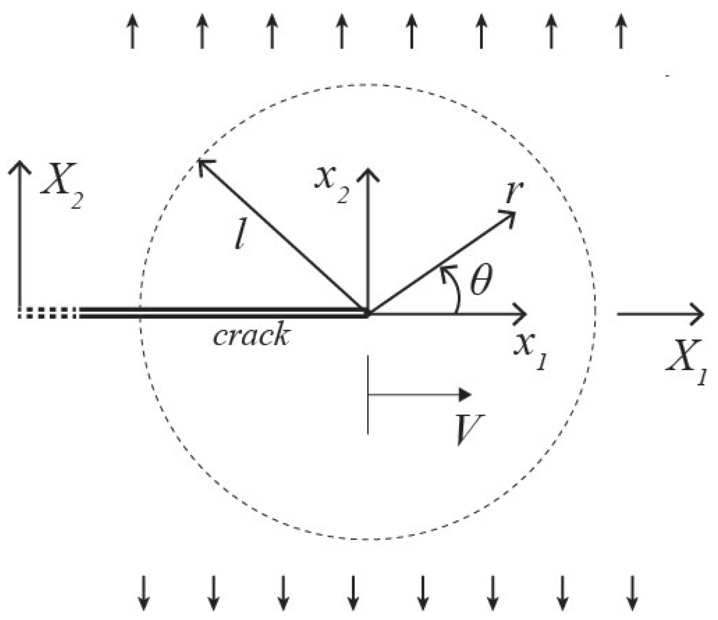
3. Asymptotic Solution for Growing Crack

We consider the plane strain steady-state problem of a Mode I crack propagated along the $X_1$-axis with the constant speed $v<c_r<c_2$ ($c_r$ is the speed of the Rayleigh waves that are studied within SGET in Refs. [14,36]). We assume that the crack propagates due to remotely applied loading (Figure 1). We seek the symmetric asymptotic solution (opening mode) around the tip of the crack in the moving coordinate system. We state that the solution for the Lamé potentials should obey the governing Equation (12) and traction-free boundary conditions at the crack faces (17) and (18) in the asymptotic sense, i.e., up to the terms that decay as $r^n$ ($n>0$) when $r\to 0$.

The solution that obeys (12) can be defined in the following form:

$$\begin{array}{cc}\hfill {\varphi }_i& =\sum _{n=-\infty }^{\infty }\left(a_{in}{\overline{r}}_i^{n}cos\left(n{\theta }_i\right)+b_{in}{I}_n\left({\overline{r}}_i\right)cos\left(n{\theta }_i\right)+{\overline{r}}_i^{n+2}\sum _{j=1}^{\infty }{c}_{inj}cos\left((n-2j){\theta }_i\right)\right),(i=1,2)\hfill \end{array}$$

(19)

$$\begin{array}{cc}\hfill r_i& =\sqrt{x_1^2+{\alpha }_i^2{x}_2^2}=r\sqrt{{cos}^2\theta +{\alpha }_i^2{sin}^2\theta },{\theta }_i=arctan\left({\alpha }_i\frac{x_2}{x_1}\right)=arctan({\alpha }_{i}tan\theta )\hfill \end{array}$$

(20)

where $r_i$ and ${\theta }_i$ are the scaled radial distance and angular coordinate that are defined with the scaling factors ${\alpha }_i=\sqrt{1-m_i^2}$ (similar scaled coordinates are introduced in the classical solution [12]); $I_n\left({\overline{r}}_i\right)$ is the modified Bessel function of the first kind; $a_{in}$ and $b_{in}$ are the independent constants that should be found from the boundary value problem; and $c_{inj}$ are the auxiliary constants that are proportional to $b_{in}$ and that should be appropriately chosen for each n-th term in series (19) so that they will asymptotically satisfy the governing equations (12). Normalization for the radial coordinate ${\overline{r}}_i=r_i/l$ is introduced to prove that all constants are nondimensional.

The classical solution for the Mode I growing crack problem [12] can be obtained as the particular case of (19), assuming that $b_{in}=c_{inj}=0$. In this case, only harmonic functions with polynomial variation along radial coordinate ($r^n$) will remain. Bessel functions in representation (19) correspond to the gradient part of the solution, and they arise due to presence of the Helmholtz operator in the governing Equation (12) (see [37]). Internal series in (12) arise as a consequence of the moving framework, while this part of solution vanishes for the quasi-static problem. The validity of the solution (19) in the case of gradient theory can be checked by its direct substitution into (12). We do not present here the derivation of this solution (these long mathematical derivations will be the subject of the forthcoming article). However, we should mention that it can be shown that auxiliary constants in (19) have the order $c_{inj}\sim b_{in}O\left(m_i^{2j}\right)$, so the amplitudes of the terms in the internal series in (19) decrease in $m_i^{2j}$ with the increase in j (since $m_i<1$). Therefore, the internal series provide clarification only for the angular distribution of solution (19). When the speed of crack propagation is not too high (low $m_i$), we can use the limited number of these terms. Thus, based on the given representation (19), we suppose to consider the following variant of the approximate solution:

$$\begin{array}{cc}\hfill {\varphi }_i& =\sum _{n=-\infty }^{\infty }{\varphi }_i^{\left(n\right)},(i=1,2)\hfill \\ \hfill {\varphi }_i^{\left(n\right)}& =a_{in}{\overline{r}}_i^{n}cos\left(n{\theta }_i\right)+b_{in}{I}_n\left({\overline{r}}_i\right)cos\left(n{\theta }_i\right)+c_{in1}{\overline{r}}_i^{n+2}cos\left((n-2){\theta }_i\right)\hfill \end{array}$$

(21)

where we neglect all the terms with constants $c_{inj}$ ($j=2,3...$) that have the order $m_i^4$ and higher. The single auxiliary constant $c_{in1}$ remaining in (21) can be found by using governing Equation (12) in the following form:

$$c_{in1}=-\frac{b_{in}{m}_i^2}{2^{n+4}(2+m_i^2)\Gamma (n+1)}$$

(22)

where $\Gamma (...)$ is the Euler gamma function, and it is also seen that the ratio of amplitudes $c_{in1}/b_{in}$ decreases with the increase in n, so the influence of these auxiliary terms will be reduced for the higher numbers of n.

To find the asymptotic solution of the problem, we should keep in series (21) only the most singular admissible terms. The order of these terms (value of n) should be chosen from the conditions of finite displacements and bounded total strain energy around the tip of the crack. From (14), it is seen that if the Lamé potentials have the order $r^n$, then the displacement field will have the order $r^{n-1}$. Therefore, all terms with $n<1$ should be excluded from the displacement solution or combined with each other to provide their vanishing when $r\to 0$ (corresponding discussion within SGET; see [37,38]). The strain energy density within SGET is evaluated accounting for the quadratic form of the strain gradients [5]. The order of the strain gradients is $r^{n-3}$ (and for the strain it is $r^{n-2}$). Therefore, the energy integrability condition in the small circular area around the crack tip requires $2(n-3)+1>-1\Rightarrow n>2$. Similar results for the quasi-static crack problems within SGET were obtained in Refs. [18,19,20].

Thus, the representation (21), together with condition $n>2$ for the nonvanishing terms around the crack tip, can provide us the appropriate asymptotic solution that approximately satisfies the governing equations in the body volume (12) and (6) for the not very high Mach numbers. Specifically, for the Mach number $m_i=0.1...0.2$, the amplitudes of the neglected angular terms in (21) will be not higher than $1...4$% of the remaining terms.

Traction-free boundary conditions at the crack faces $\theta =\pi$ (17) and (18) allow us to find the admissible value of factor n and some of the constants $a_{in}$, $b_{in}$ in (21). Following the standard procedure for the crack tip field problems [12,19], we should use the condition of the zero determinant of the system of boundary conditions (17) and (18) to find n. Substituting ${\varphi }_i^{\left(n\right)}$ (21) into (14)–(16) and the result into the boundary conditions (17) and (18) at $\theta =\pi$, one can find that the determinant of the obtained system is proportional to ${sin}^2\left(2n\pi \right)$. Therefore, this determinant will be zero if $n=p/2$ ($p=0,\pm 1,\pm 2...$). Based on the energy integrability condition, we find then that the leading terms $r^n$ in the asymptotic solution for the Lamé potentials should have the order $n=5/2>2$, and for the displacement field, we obtain the asymptotics $r^{n-1}=r^{3/2}$ (similarly to known solutions for the static SGET problems [18,19,20]).

Thus, we should extract all terms with asymptotic behavior $r^{5/2}$ from representation (21). Notably, such terms will persist not only in the function ${\varphi }_i^{(5/2)}$, but also in the functions ${\varphi }_i^{n/2}$, $n=5-2p$ ($p=1,2...$) that follow from the series expansion for the modified Bessel function $I_n\left({\overline{r}}_i\right)$. At the same time, for the functions ${\varphi }_i^{(n/2)}$ with index $n\le 1$, we obtain the high-order singular components in the displacement field that should be avoided by the appropriate choice of constants $a_{in}$ and $b_{in}$ (a similar analysis within the generalized Flamant problem was presented recently in Ref. [37]). Based on the analysis of the behavior of functions ${\varphi }_i^{\left(n\right)}$ around $r=0$, we found that the following terms should remain for the asymptotic solution:

$${\varphi }_i={\varphi }_i^{(1/2)}+{\varphi }_i^{(5/2)}+{\varphi }_i^{\left(0\right)}+{\varphi }_i^{\left(2\right)},(i=1,2)$$

(23)

whose regularity around $r=0$ can be provided by the following choice of constants:

$$b_{i1}=-\sqrt{\frac{\pi }{2}}{a}_{i1}$$

(24)

where for the shortness, we adopt the following notation for the fractional indexes: “n” instead of “n/2” for odd values of n (i.e., $a_{i1}$ means $a_{i(1/2)}$, $b_{i1}$ means $b_{i(1/2)}$, etc.). This notation is also used in the following derivations.

Note that apart from the mentioned functions in (23), all functions ${\varphi }_i^{(n/2)}$ with the negative index $n/2<0$ also contain the terms with behavior $\sim r^{3/2}$. However, all these functions allow for regularity for the displacement field around $r=0$ only if both constants are zero: $a_{in}=b_{in}=0$. Therefore, these functions are excluded from the solution. The high-order terms with $n>5/2$ are also out of consideration within the asymptotic solution for the crack tip fields only.

Separately, within SGET, one should consider the case that corresponds to the particular solution with vanishing strain gradients around the crack tip. Such a solution can be obtained by using the Lamé potentials ${\varphi }_1^{\left(0\right)}$, ${\varphi }_i^{\left(2\right)}$ that produce the displacement field with asymptotic behavior $\sim r^1$. For this case ($n=0$ and $n=2$), the energy integrability condition can be relaxed, and functions ${\varphi }_1^{\left(0\right)}$, ${\varphi }_i^{\left(2\right)}$ can be included in (23). These lower-order terms can be related to the so-called generalized T-stress field that also arises in the quasi-static SGET solutions [18,19,20].

Substituting definitions for ${\varphi }_i^{\left(n\right)}$ (21) into (23) and taking into account (24), one can obtain the final form of the Lamé potentials. Using these potentials in (14) and evaluating the limit at $r\to 0$, one can find the SGET asymptotic solution for the displacement field around the tip of the propagated crack in the following form:

$$\begin{array}{cc}\hfill {\overline{u}}_r& =\overline{r}{S}_0{\beta }_{10}+\overline{r}\sum _{i=1}^2{S}_i{\beta }_{i1}cos2{\theta }_i+m_2^2{F}_r(\overline{r},{\theta }_i)\hfill \\ \hfill & +{\overline{r}}^{3/2}\sum _{i=1}^2\left(a_{i1}{\kappa }_{i1}cos\frac{{\theta }_i}{2}+c_{i11}{\kappa }_{i2}cos\frac{3{\theta }_i}{2}+(a_{i5}{\kappa }_{i3}+b_{i5}{\kappa }_{i4})cos\frac{5{\theta }_i}{2}\right)\hfill \\ \hfill {\overline{u}}_{\theta }& =-\overline{r}\sum _{i=1}^2{S}_i{\beta }_{i2}sin2{\theta }_i+m_1^2{F}_{\theta }(\overline{r},{\theta }_i)\hfill \\ \hfill & +{\overline{r}}^{3/2}\sum _{i=1}^2\left(a_{i1}{\kappa }_{i5}sin\frac{{\theta }_i}{2}+c_{i11}{\kappa }_{i6}sin\frac{3{\theta }_i}{2}+(a_{i5}{\kappa }_{i7}+b_{i5}{\kappa }_{i8})sin\frac{5{\theta }_i}{2}\right)\hfill \end{array}$$

(25)

where $\overline{r}=r/l$, ${\overline{u}}_r=u_r/l$, ${\overline{u}}_{\theta }=u_{\theta }/l$ are the normalized radial distance and components of the displacement field, respectively; $c_{in1}$ are defined by (22); ${\kappa }_{ij}$, ${\beta }_{ij}$ are the functions of the angular coordinate, whose explicit form is given in Appendix A; the amplitudes for the lower-order crack tip fields are defined by $S_0=b_{10}/2$, $S_1=2a_{12}+b_{12}/4+2c_{101}$, $S_2=2a_{22}+b_{22}/4-2c_{201}$; and functions $F_r$, $F_{\theta }$ are introduced to define the terms that arise only in the steady-state problem and that vanish in the quasi-static limit $m_i=0$ (see Appendix A).

Solution (25) contains six unknown constants that define the leading terms: $a_{11}$, $a_{15}$, $b_{15}$, $a_{21}$, $a_{25}$, $b_{25}$. Three of these constants (e.g., $a_{11}$, $a_{21}$, $b_{25}$) can be determined from the boundary conditions (17) and (18) to provide their fulfilment in the asymptotic sense. The representation for these constants can be easily found in analytical form by using a symbolic algebra system, and they are not presented here for clarity. Additionally, one should consider the low-order fields defined by constants $a_{ij}$, $b_{ij}$ ($i=1,2$, $j=0,2$) that combine together into three amplitudes $S_i$ ($i=0,1,2$) in solution (25). The boundary condition for traction $t_{\theta }$ gives a single additional nontrivial relation between these constants that can be fulfilled by the appropriate choice of one of them (e.g., $b_{20}$). The remaining constants left unspecified by the asymptotic analysis.

From (25), it is seen that in contrast to the classical elasticity solution, in SGET, we have the smooth opening profile that varies according to the leading terms order $\sim r^{3/2}$. Therefore, the strain field and the stresses that can be found by using the generalized Hooke’s law (5) vary as $r^{1/2}$, and they are bounded at the tip of crack. The double stresses and tractions are singular and proportional to $r^{-1/2}$ and $r^{-3/2}$, respectively. Analyses of the realized deformations and distribution of stresses and tractions in the developed solution are presented in the next section.

As it follows from the presented derivations, the formal reason for the obtained regularized SGET solution for the crack tip fields is the condition of the bounded total strain energy in the vicinity of the crack tip. From the physical point of view, the smoothed opening profile may arise due to the influence of degradation mechanisms (microvoiding, microcracking) around the crack tip in quasi-brittle materials [39]. Such effects are usually described within the nonlinear models of cohesion cracks with prescribed traction–separation lows [40]. The use of high-grade theories allows us to consider the phenomenological description of cohesive-zone effects, even within the linear formulation [20,27].

Notably, the known form of the quasi-static solution for the crack tip fields within SGET can be obtained from (25), taking the limit for zero speed of crack propagation $v\to 0$, $m_i\to 0$ (see Appendix A).

4. Results and Discussion

For the examples of numerical calculations, let us clarify the physical meaning and possible values of the constants $S_0$, $S_1$, $S_2$, $a_{15}$, $a_{25}$, $b_{15}$ that remain in solutions (23)-(25). From (21), it can be seen that the constants $a_{15}$, $b_{15}$ are related to the scalar Lamé potential ${\varphi }_1$, and therefore, they define the dilatational strain field around the tip of the crack. Conversely, constant $a_{25}$ is related to the vector potential ${\varphi }_2$ and defines the rotations in the vicinity of a crack. Similar observations for two constants that persist in the asymptotic solution for the stationary cracks within SGET are given in Ref. [18]. Note that constant $b_{15}$ stays before the modified Bessel function in Equation (21), and mostly defines the high-order effects in the distribution of dilatation (interconnected with terms $\sim r^{7/2}$ and higher). The influence of $b_{15}$ on the crack tip field is negligible, and in further examples of calculation, we will use $b_{15}=0$, so only two independent amplitudes of the leading terms $a_{15}$ and $a_{25}$ will be considered.

The amplitudes of the lower-order crack-tip fields $S_i$ in the case of the static problem ($m_i=0$) have the physical meaning of the constant normal strains that can be represented in the Cartesian coordinates as ${\epsilon }_{11}=S_0+S_1+S_2$ and ${\epsilon }_{22}=S_0-S_1-S_2$ (see [18]). These components of the asymptotic solution do not make a contribution to the energy release rate and to the crack tip open displacement [18,19]. For the nonzero speed of crack propagation constants, $S_i$ corresponds to the distorted lower-order strain fields around the growing crack, whose distribution is defined by functions ${\beta }_{ij}$ (Appendix A). For the examples of calculations, we will define the lower-order crack tip fields, assuming that they correspond to the uniform tension along the $x_2$-axis in the quasi-static limit:

$${\epsilon }_{22}=-{\epsilon }_{11}/\nu ={\epsilon }_0$$

Then, the values of amplitudes can be chosen as

$$S_0={\epsilon }_0(1-\nu )/2,S_1=S_2=-{\epsilon }_0(1+\nu )/4$$

which can be provided by using the following definitions for the constants of the Lamé potentials (21):

$$b_{10}={\epsilon }_0(1-\nu ),a_{12}=a_{22}=-{\epsilon }_0(1+\nu )/8,b_{12}=b_{22}=0$$

and the last constant $b_{20}$ is used to provide the fulfilment of traction-free boundary conditions. Note that the case of the loaded crack faces can be also considered, and the corresponding boundary conditions can be satisfied by the appropriate choice of constants $b_{12}$, $b_{22}$, $b_{20}$, though this case is out of consideration in this study.

Thus, for the following analysis, we can retain only four nondimensional parameters: Poisson ratio $\nu$, Mach number $m_2$ (or $m_1$), and the ratios between the amplitudes of local dilatation and rotation fields to the amplitude of uniform tension denoted by $k_{\theta }=-a_{15}/{\epsilon }_0$ and $k_{\omega }=-a_{25}/{\epsilon }_0$, respectively. In definitions for $k_{\theta }$ and $k_{\omega }$, we use the minus sign due to the condition of the open mode-I crack that requires $u_{\theta }(r,\pi )<0$ when ${\epsilon }_0>0$.

In the following, unless otherwise stated, we use the values of Poisson’s ratio $\nu =0.3$, Mach number $m_2=0.1$, and amplitude ratios $k_{\theta }=0.1$ and $k_{\omega }=0.1$ with the prescribed uniform tension amplitude ${\epsilon }_0=1$ (some of these quantities are varied, and this will be denoted on the plots). All spatial dimensions, coordinates, and displacements are normalized with respect to the length scale parameter l. Stresses and surface tractions are normalized with respect to the Young’s modulus of material multiplied with the prescribed amplitude of tensile strain ${\epsilon }_0$. These normalized quantities will be denoted with a hat symbol (${\widehat{t}}_{\theta }$, etc.). The stresses and surface tractions are calculated by using given solution (21) and (23) and relations (14)–(17). All evaluations are performed by using the initial definition for the solution with Bessel functions (21) to provide the correct values of their derivatives and taking into account definitions for the scaled coordinates (20). Asymptotic solutions for the crack tip fields are found for the resulting relations using the series expansion for the Bessel functions around $r=0$, and retaining only the leading terms.

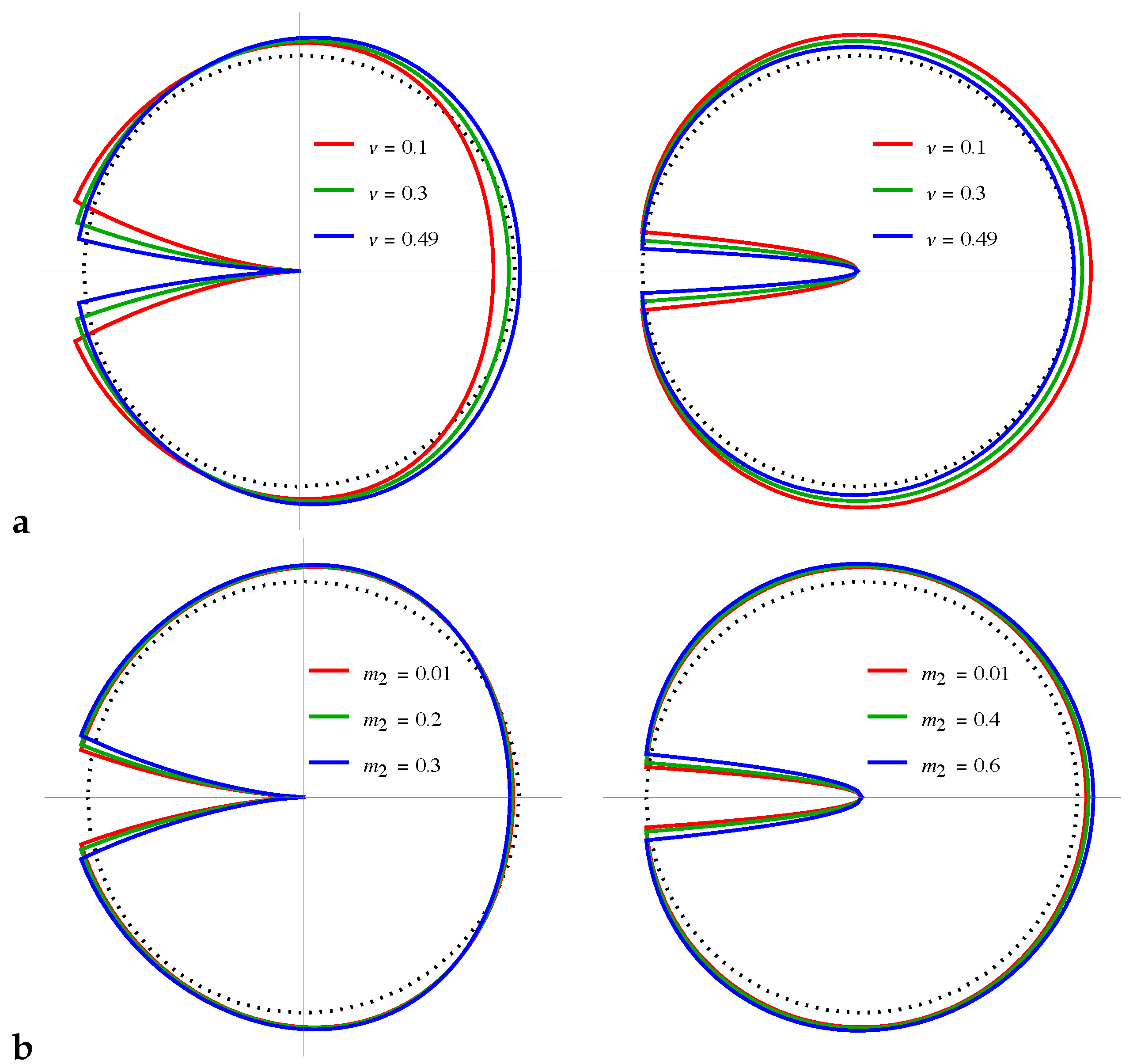
Illustrations for the displacement field that is realized in the vicinity of a crack are presented in Figure 2. Here, we show the deformations of a small circle with radius $r=0.1l$ around the tip of a crack in SGET (left) and in classical [12] (right) solutions. It can be seen that in contrast to the classical solution with $r^{1/2}$ asymptotics, the smooth closure profile is realized in SGET, which can be related to the presence of the fracture process zone in quasi-brittle materials [20]. The dependence of crack tip open displacement on Poisson’s ratio and the Mach number are similar in both solutions: the opening amplitude becomes higher for the lower values of Poisson’s ratio and for the high Mach number (though in the classical solution, we have to use higher values of $m_2$ to obtain a more visible effect). At the same time, the deformed state ahead of the crack tip varies differently in the classical and SGET solutions. In the classical solution, a tension along the $x_1$-axis always arises in this zone. In SGET, there arises a compression along the $x_1$-axis ahead of the crack tip for the low values of Poisson’s ratio and for all considered values of the Mach number.

The influence of the amplitude ratios $k_{\theta }$, $k_{\omega }$ on the displacement field around the crack tip is shown in Figure 3. It can be seen that the increase in dilatational amplitude $k_{\theta }$ results in a higher crack opening and a more intensive compression ahead of the crack tip (Figure 3a). The influence of the rotational amplitude is much less pronounced, and can be seen only for relatively large values of $k_{\omega }$, which results in the higher curvature of the deformed crack face and additional distortion along the $x_1$ axis of the plotted circles (Figure 3b). The negative values of $k_{\omega }$ lead to the double curvature of the crack face (red curve in Figure 3b). Note that in the vicinity of a crack tip, the change in $k_{\omega }$ does not influence the crack tip open displacement (all curves coincide at the crack tip in Figure 3b), so the rotational effects in tbe SGET asymptotic solution could be negligible for Mode-I loading.

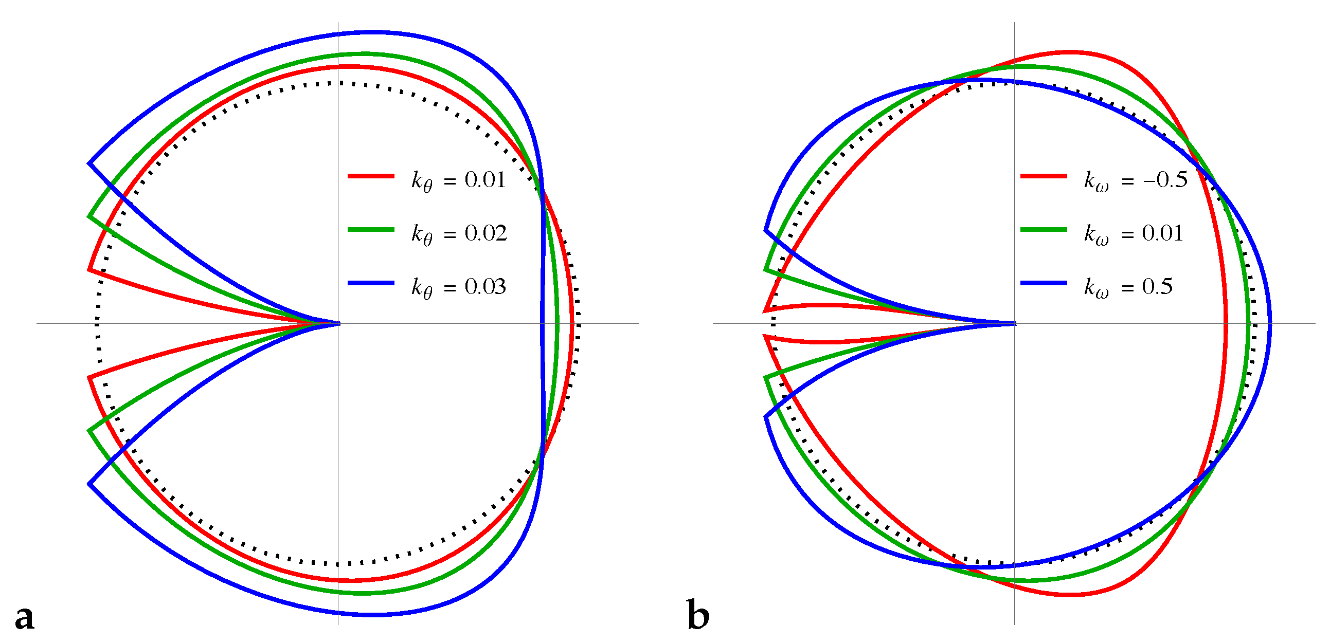
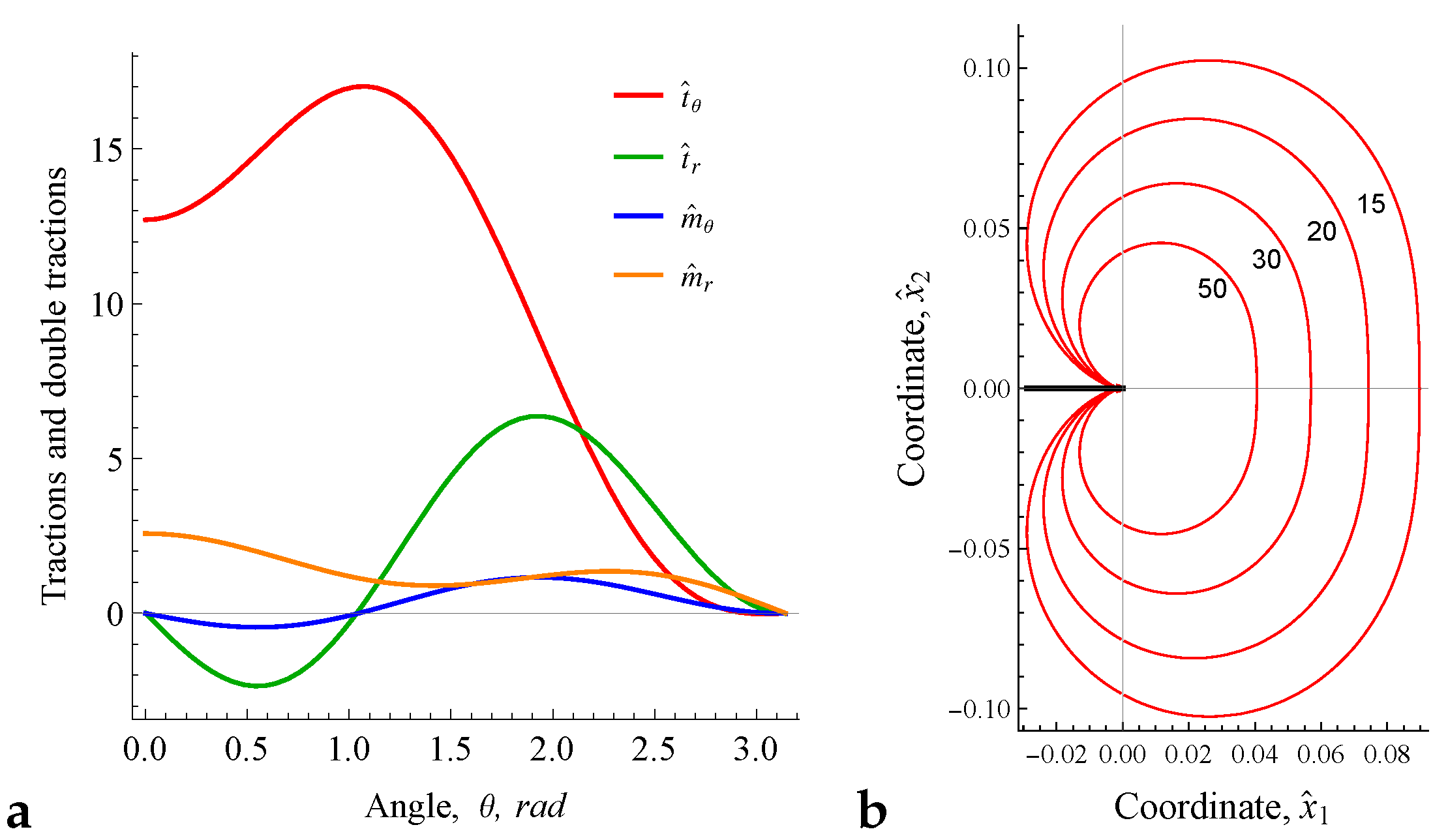
An illustration of the fulfilment of the traction-free boundary conditions by the developed asymptotic solution is presented in Figure 4. In Figure 4a, we show the typical angular distribution of normalized tractions (17) and double tractions (18) that take zero values at the crack face $\theta =\pi$. The contour plots for the in-plane distribution of normalized hoop traction $t_{\theta }$ are presented in Figure 4b. This traction has a singular behavior $\sim r^{-3/2}$ and growth rapidly close to the crack tip. 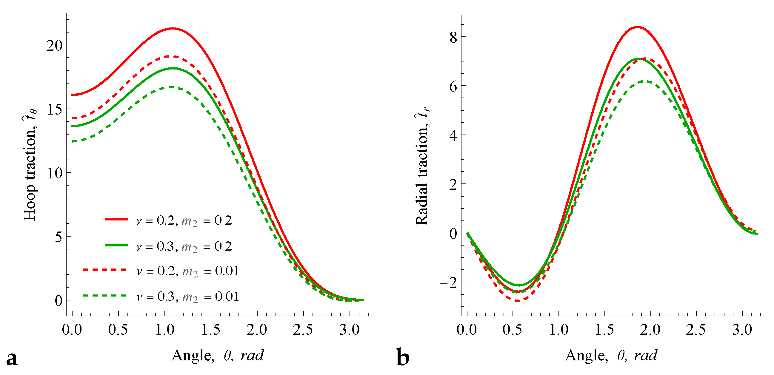Note that the angular distribution and dependence on the Mach number of the tractions in the SGET solution are very similar to those in classical solutions (Figure 5), though their definitions are much more complicated (17). Hoop traction $t_{\theta }$ has a maximum at about $\theta =60$ deg. (Figure 5a), where the radial traction $t_r$ changes the sign (Figure 5b). Similarly to the classical theory, in SGET, the maximum values of $t_{\theta }$ and $t_r$ increase with the increase in Mach number (solid lines in Figure 5).

Recently, it was proposed that the nominal strength of materials with cracks can be evaluated within SGET based on the regularized solutions for the stresses [28,41]. In SGET, stress and strain are regular at the crack tip, and one can use their finite values to define the criteria of the crack growth initiation and the direction of growth. A description of the known experimental data for the quasi-static and fatigue tests with brittle and quasi-brittle materials within SGET is given in Refs. [27,28,41]. It was shown that the size effect for the nominal strength and transition between short and long crack regimes can be described within SGET [27,28]. Thus, in this study, we evaluate the effects that can be captured by using the regularized asymptotic solution for the steady-state crack in SGET. 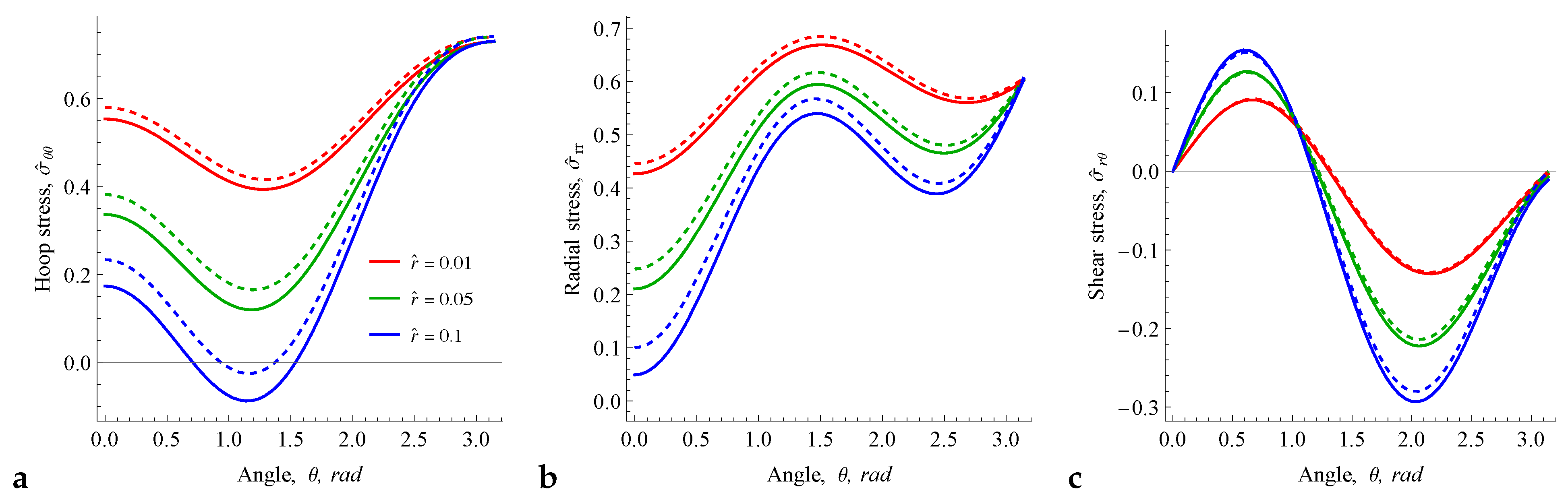Note that since the leading terms for stresses (5) vary as $\sim r^{1/2}$, they vanish exactly at the crack tip, and only the low-order fields with the terms $\sim r^0$ play a role in the fracture initiation if we adopt the viewpoint of regularized analysis within SGET. This is illustrated in Figure 5 and Figure 6. In Figure 6, we show the angular distribution of stress tensor components at different distances from the crack tip. It is seen that all components vary differently in the full range of angles, though from the side of the crack face ($\theta =\pi$), they reach the constant values that are not affected by the distance $\widehat{r}$ at which they are evaluated. Note that these nonzero stresses at crack faces are not restricted by the formulation of SGET, since the tractions (17) are defined with additional terms related to the gradients of double stresses (these terms are equilibrated by the stresses so that the traction-free boundary conditions are fulfilled, as can be seen in Figure 3 and Figure 4). Thus, the non-zero stresses at the crack faces can be treated as the cohesive forces that naturally arise in the SGET solutions for crack problems [27].

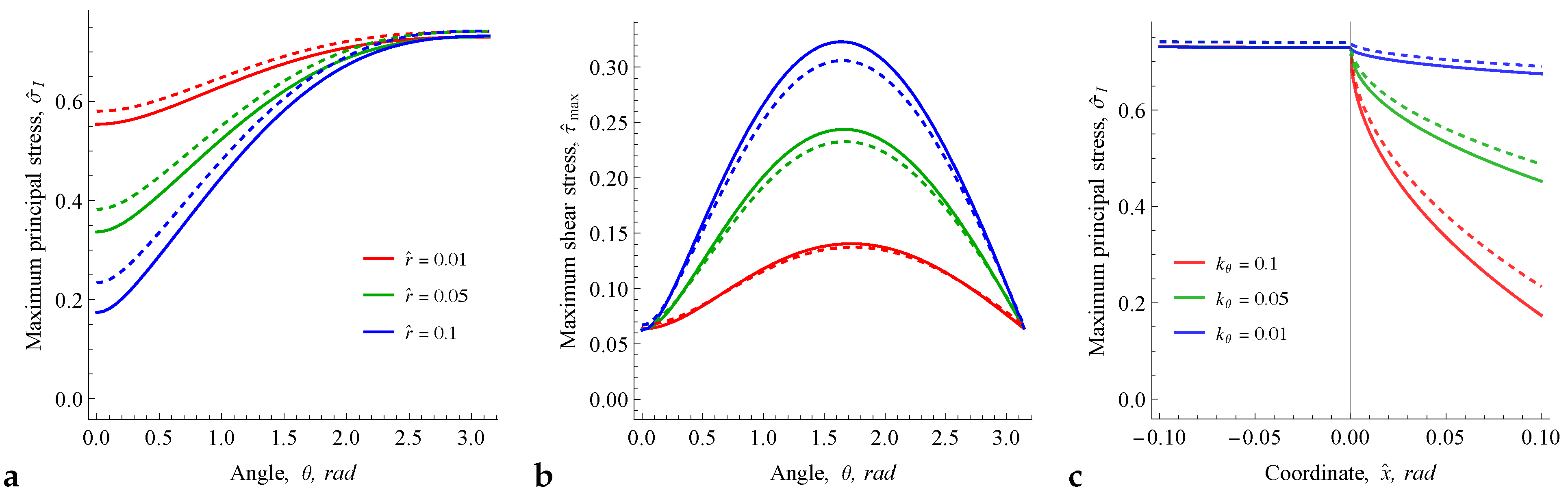
Evaluating the normalized maximum principal stress ${\widehat{\sigma }}_I$ and maximum shear stress ${\widehat{\tau }}_{max}$ according to their standard definitions with components of stress tensor $\sigma$ (5), we can check the criterion for the direction of the crack growth within the regularized analysis. In Figure 7a,b, we show the angular distribution of ${\widehat{\sigma }}_I$ and ${\widehat{\tau }}_{max}$. It is seen that the maximum principal stress always arises at the crack tip from the side of the crack face ($\theta =\pi$), while the maximum stress has lower values and has a maximum at about $\theta =\pi /2$. Therefore, adopting the maximum principal stress criterion for the direction of crack growth, we found that the crack should propagate straightly along the $x_1$-axis direction with the permanent destruction of cohesive bonds in the fracture process zone in the crack tip at $\theta =\pi /2$, where the maximum principal stress should reach the critical values of the cohesive stress. Note that a similar observation is given based on the atomistic simulations in Ref. [31], where it was shown that the maximum normal stress arises behind the position of the virtual crack tip inside the cohesive zone. Note that the obtained SGET results do not contain paradoxes of the classical elasticity solution, where the assumed straight propagation of the crack cannot be validated by the criteria of the crack propagation direction [12].

Ahead of the crack tip, the maximum principal stress decreases, and the rate of its decay is defined primarily by the value of the dilatation amplitude ratio $k_{\theta }$ (see Figure 7c). The maximum values of ${\widehat{\sigma }}_I$ do not depend on $k_{\theta }$ and are defined by the low-order crack tip fields, which are reduced in the presented analysis to the amplitude of tensile strain ${\epsilon }_0$. Moreover, the level of maximum principal stress depends on the Mach number. It is interesting to note that ${\widehat{\sigma }}_I$ and hoop stress ${\widehat{\sigma }}_{\theta \theta }$ decrease with the increase in Mach number (compare solid lines and dashed lines in Figure 6a,c). Thus, within the regularized analysis, we can state that the dynamic toughness of materials governed by SGET is predicted to be higher than those under quasi-static loading. Note that such effects have been observed in experiments with quasi-brittle glassy polymers [42,43], where the toughness was higher for the higher speeds of crack propagation (notably, that inverse dependences arise in the purely brittle processes [12,44]). This effect was explained by the craze-widening process and described by the rate-dependent cohesive models [42]. As can be seen, from the high-grade continuum point of view, the increase in dynamic toughness with propagation speed can be naturally described within the regularized SGET solutions. However, in the presented analysis, we used not very high Mach numbers to provide the accuracy of the approximate solution (21).

5. Conclusions

In this paper, we derived an asymptotic solution for the problem of steady-state propagation of Mode-I cracks in the quasi-brittle materials governed by SGET. A simplified variant of SGET and the particular case of the same values of the elastic and microinertia length scale parameters were considered. The form of asymptotic solution was derived based on the Lamé potential approach, and its approximate variant for the moderate values of Mach number were used for the analysis of the deformations and the stress state around the moving crack tip. It was shown that the typical smooth crack opening profile with "cohesive zone" effects are predicted by the dynamic solution of SGET. Moreover, from the given assessments, it follows the possibility for the description of the straight direction of the Mode-I crack growth without paradoxes of classical theory. The increases in the dynamic fracture toughness of the quasi-brittle material that were observed in the experiments can be also described within the regularized analysis and maximum principal stress criterion of SGET.

The presented results are given for the not very high Mach numbers of crack propagation and particular relations between the length scale parameters of SGET. Specifically, the main limitation of the presented results is the assumption of the same values of the length scale parameters for the strain (l) and for the inertia (g) gradient effects and the limited number of terms used in the definition of the angular distribution of asymptotic solution (21). Therefore, in future work, the presented analysis should be extended for the subsonic and intersonic regimes. The more general constitutive equations of SGET should be also considered and compared to the full-field numerical simulations.

References

1. Placidi, L.; Greco, L.; Bucci, S.; Turco, E.; Rizzi, N.L. A second gradient formulation for a 2D fabric sheet with inextensible fibres. Z. Angew. Math. Phys. 2016, 67, 1–24. [Google Scholar] [CrossRef]
2. Shveykin, A.; Romanov, K.; Trusov, P. Some Issues with Statistical Crystal Plasticity Models: Description of the Effects Triggered in FCC Crystals by Loading with Strain-Path Changes. Materials 2022, 15, 6586. [Google Scholar] [CrossRef]
3. Fleck, N.; Hutchinson, J. A reformulation of strain gradient plasticity. J. Mech. Phys. Solids 2001, 49, 2245–2271. [Google Scholar] [CrossRef]
4. Ghiba, I.D.; Neff, P.; Madeo, A.; Placidi, L.; Rosi, G. The relaxed linear micromorphic continuum: Existence, uniqueness and continuous dependence in dynamics. Math. Mech. Solids 2015, 20, 1171–1197. [Google Scholar] [CrossRef]
5. Mindlin, R.D. Micro-structure in linear elasticity. Arch. Ration. Mech. Anal. 1964, 16, 51–78. [Google Scholar] [CrossRef]
6. Placidi, L.; Barchiesi, E. Energy approach to brittle fracture in strain-gradient modelling. Proc. R. Soc. Math. Phys. Eng. Sci. 2018, 474, 20170878. [Google Scholar] [CrossRef] [PubMed]
7. Makvandi, R.; Abali, B.E.; Eisenträger, S.; Juhre, D. A strain gradient enhanced model for the phase-field approach to fracture. PAMM 2021, 21, e202100195. [Google Scholar] [CrossRef]
8. Gutkin, M.Y.; Aifantis, E. Dislocations in the theory of gradient elasticity. Scr. Mater. 1999, 40, 559–566. [Google Scholar] [CrossRef]
9. Po, G.; Lazar, M.; Seif, D.; Ghoniem, N. Singularity-free dislocation dynamics with strain gradient elasticity. J. Mech. Phys. Solids 2014, 68, 161–178. [Google Scholar] [CrossRef]
10. Rosi, G.; Placidi, L.; Auffray, N. On the validity range of strain-gradient elasticity: A mixed static-dynamic identification procedure. Eur. J. -Mech.-A/Solids 2018, 69, 179–191. [Google Scholar] [CrossRef]
11. Shekarchizadeh, N.; Laudato, M.; Manzari, L.; Abali, B.E.; Giorgio, I.; Bersani, A.M. Parameter identification of a second-gradient model for the description of pantographic structures in dynamic regime. Z. FÜR Angew. Math. Und Phys. 2021, 72, 1–24. [Google Scholar] [CrossRef]
12. Ravi-Chandar, K. Dynamic Fracture; Elsevier: Amsterdam, The Netherlands, 2004. [Google Scholar]
13. Nielsen, K.L.; Niordson, C.F.; Hutchinson, J.W. Strain gradient effects on steady state crack growth in rate-sensitive materials. Eng. Fract. Mech. 2012, 96, 61–71. [Google Scholar] [CrossRef]
14. Gourgiotis, P.; Piccolroaz, A. Steady-state propagation of a mode II crack in couple stress elasticity. Int. J. Fract. 2014, 188, 119–145. [Google Scholar] [CrossRef]
15. Radi, E. Strain-gradient effects on steady-state crack growth in linear hardening materials. J. Mech. Phys. Solids 2003, 51, 543–573. [Google Scholar] [CrossRef]
16. Mishuris, G.; Piccolroaz, A.; Radi, E. Steady-state propagation of a Mode III crack in couple stress elastic materials. Int. J. Eng. Sci. 2012, 61, 112–128. [Google Scholar] [CrossRef]
17. Morini, L.; Piccolroaz, A.; Mishuris, G.; Radi, E. On fracture criteria for dynamic crack propagation in elastic materials with couple stresses. Int. J. Eng. Sci. 2013, 71, 45–61. [Google Scholar] [CrossRef]
18. Aravas, N.; Giannakopoulos, A. Plane asymptotic crack-tip solutions in gradient elasticity. Int. J. Solids Struct. 2009, 46, 4478–4503. [Google Scholar] [CrossRef]
19. Gourgiotis, P.; Georgiadis, H. Plane-strain crack problems in microstructured solids governed by dipolar gradient elasticity. J. Mech. Phys. Solids 2009, 57, 1898–1920. [Google Scholar] [CrossRef]
20. Sciarra, G.; Vidoli, S. Asymptotic fracture modes in strain-gradient elasticity: Size effects and characteristic lengths for isotropic materials. J. Elast. 2013, 113, 27–53. [Google Scholar] [CrossRef]
21. Lazar, M.; Polyzos, D. On non-singular crack fields in Helmholtz type enriched elasticity theories. Int. J. Solids Struct. 2015, 62, 1–7. [Google Scholar] [CrossRef]
22. Solyaev, Y. Semi-analytical solution for the Lamb’s problem in second gradient elastodynamics. Wave Motion 2023, 120, 103145. [Google Scholar] [CrossRef]
23. Placidi, L.; El Dhaba, A.R. Semi-inverse method à la Saint-Venant for two-dimensional linear isotropic homogeneous second-gradient elasticity. Math. Mech. Solids 2017, 22, 919–937. [Google Scholar] [CrossRef]
24. Eremeyev, V.A.; Scerrato, D.; Konopińska-Zmysłowska, V. Ellipticity in couple-stress elasticity. Z. Angew. Math. Phys. 2023, 74, 18. [Google Scholar] [CrossRef]
25. Morini, L.; Piccolroaz, A.; Mishuris, G. Remarks on the energy release rate for an antiplane moving crack in couple stress elasticity. Int. J. Solids Struct. 2014, 51, 3087–3100. [Google Scholar] [CrossRef]
26. Gourgiotis, P.; Georgiadis, H. The problem of sharp notch in couple-stress elasticity. Int. J. Solids Struct. 2011, 48, 2630–2641. [Google Scholar] [CrossRef]
27. Vasiliev, V.; Lurie, S.; Solyaev, Y. New approach to failure of pre-cracked brittle materials based on regularized solutions of strain gradient elasticity. Eng. Fract. Mech. 2021, 258, 108080. [Google Scholar] [CrossRef]
28. Askes, H.; Susmel, L. Understanding cracked materials: Is linear elastic fracture mechanics obsolete? Fatigue Fract. Eng. Mater. Struct. 2015, 38, 154–160. [Google Scholar] [CrossRef]
29. Fan, T. Moving Dugdale model. Z. Angew. Math. Phys. Zamp 1987, 38, 630–641. [Google Scholar] [CrossRef]
30. Wang, F.; Zhu, Z.; Wang, M.; Qiu, H.; Zhou, L.; Liu, R.; Ying, P. Investigation of mixed-mode I/II fracture under impact loading using Split-Hopkinson pressure bar. Appl. Sci. 2020, 10, 7149. [Google Scholar] [CrossRef]
31. Lee, G.H.; Kim, J.H.; Beom, H.G. Cohesive zone modeling of crack propagation in FCC single crystals via atomistic simulations. Met. Mater. Int. 2021, 27, 584–592. [Google Scholar] [CrossRef]
32. Khakalo, S.; Niiranen, J. Form II of Mindlin’s second strain gradient theory of elasticity with a simplification: For materials and structures from nano-to macro-scales. Eur. J. -Mech.-A/Solids 2018, 71, 292–319. [Google Scholar] [CrossRef]
33. Askes, H.; Aifantis, E.C. Gradient elasticity in statics and dynamics: An overview of formulations, length scale identification procedures, finite element implementations and new results. Int. J. Solids Struct. 2011, 48, 1962–1990. [Google Scholar] [CrossRef]
34. Dell’Isola, F.; Sciarra, G.; Vidoli, S. Generalized Hooke’s law for isotropic second gradient materials. Proc. R. Soc. Math. Phys. Eng. Sci. 2009, 465, 2177–2196. [Google Scholar] [CrossRef]
35. Polizzotto, C. A unifying variational framework for stress gradient and strain gradient elasticity theories. Eur. J. -Mech.-A/Solids 2015, 49, 430–440. [Google Scholar] [CrossRef]
36. Gourgiotis, P.A. Shear crack growth in brittle materials modeled by constrained Cosserat elasticity. J. Eur. Ceram. Soc. 2018, 38, 3025–3036. [Google Scholar] [CrossRef]
37. Solyaev, Y.; Lurie, S.; Altenbach, H.; dell’Isola, F. On the elastic wedge problem within simplified and incomplete strain gradient elasticity theories. Int. J. Solids Struct. 2022, 234, 111433. [Google Scholar] [CrossRef]
38. Lurie, S.A.; Volkov-Bogorodsky, D.B.; Vasiliev, V.V. A new approach to non-singular plane cracks theory in gradient elasticity. Math. Comput. Appl. 2019, 24, 93. [Google Scholar] [CrossRef]
39. Bažant, Z.P.; Le, J.L.; Salviato, M. Quasibrittle Fracture Mechanics and Size Effect: A First Course; Oxford University Press: Oxford, UK, 2021. [Google Scholar]
40. Xiao, Q.; Karihaloo, B.L. Asymptotic fields at frictionless and frictional cohesive crack tips in quasibrittle materials. J. Mech. Mater. Struct. 2006, 1, 881–910. [Google Scholar] [CrossRef]
41. Vasiliev, V.; Lurie, S.; Salov, V. Estimation of the strength of plates with cracks based on the maximum stress criterion in a scale-dependent generalized theory of elasticity. Phys. Mesomech. 2019, 22, 456–462. [Google Scholar] [CrossRef]
42. Zhou, F.; Molinari, J.F.; Shioya, T. A rate-dependent cohesive model for simulating dynamic crack propagation in brittle materials. Eng. Fract. Mech. 2005, 72, 1383–1410. [Google Scholar] [CrossRef]
43. Joudon, V.; Portemont, G.; Lauro, F.; Bennani, B. Experimental procedure to characterize the mode I dynamic fracture toughness of advanced epoxy resins. Eng. Fract. Mech. 2014, 126, 166–177. [Google Scholar] [CrossRef]
44. Wang, F.; Wang, M.; Mousavi Nezhad, M.; Qiu, H.; Ying, P.; Niu, C. Rock dynamic crack propagation under different loading rates using improved single cleavage semi-circle specimen. Appl. Sci. 2019, 9, 4944. [Google Scholar] [CrossRef]
Figure 1. Illustration for the growing crack problem with global and local (moving) coordinate systems. Opening mode under remotely applied loading is considered. Solution is found in the vicinity of a crack tip, where r ¯ 1 , i.e., r l .
Applsci 13 06333 g001
Figure 2. Influence of Poisson’s ratio (a) and Mach number (b) of the deformations of small circles around the crack tip in SGET (left) and classical (right) asymptotic steady-state solutions.
Applsci 13 06333 g002
Figure 3. Influence of dilatational (a) and rotational (b) amplitudes on the deformed state around the tip of crack.
Applsci 13 06333 g003
Figure 4. Typical dependence of normalized tractions and double tractions on angular coordinate (a) and in-plane distribution of normalized hoop traction t ^ θ ((b), crack is shown by thick black line) in SGET asymptotic solution.
Applsci 13 06333 g004
Figure 5. Angular distribution of normalized hoop traction (a) and radial traction (b) for different values of Mach number and Poisson’s ratio.
Applsci 13 06333 g005
Figure 6. Angular distribution of normalized stress components σ ^ θ θ (a), σ ^ r θ (b), σ ^ r r (c) evaluated at different distances from the crack tip and for the values of Mach number m 2 = 0.2 (solid lines) and m 2 = 0.01 (dashed lines).
Applsci 13 06333 g006
Figure 7. Angular distribution of normalized maximum principal stress (a) and maximum shear stress (b) and distribution of the normalized maximum principal stress along the crack propagation direction (along x 1 at x 2 = 0 ) for different values of amplitude ratio k θ (c). The values of Mach number are m 2 = 0.2 (solid lines) and m 2 = 0.01 (dashed lines).
Applsci 13 06333 g007
Disclaimer/Publisher’s Note: The statements, opinions and data contained in all publications are solely those of the individual author(s) and contributor(s) and not of MDPI and/or the editor(s). MDPI and/or the editor(s) disclaim responsibility for any injury to people or property resulting from any ideas, methods, instructions or products referred to in the content.