DRFENet: An Improved Deep Learning Neural Network via Dilated Skip Convolution for Image Denoising Application

Abstract

Deep learning technology dominates current research in image denoising. However, denoising performance is limited by target noise feature loss from information propagation in association with the depth of the network. This paper proposes a Dense Residual Feature Extraction Network (DRFENet) combined with a Dense Enhancement Block (DEB), a Residual Dilated Block (RDB), a Feature Enhancement Block (FEB), and a Simultaneous Iterative Reconstruction Block (SIRB). The DEB uses our proposed interval transmission strategy to enhance the extraction of noise features in the initial stage of the network. The RDB module uses a combination strategy of concatenated dilated convolution and a skip connection, and the local features are amplified through different perceptual dimensions. The FEB enhances local feature information. The SIRB uses an attention block to learn the noise distribution while using residual learning (RL) technology to reconstruct a denoised image. The combination strategy in DRFENet makes the neural network deeper to obtain higher fine-grained image information. We respectively examined the performance of DRFENet in gray image denoising on datasets BSD68 and SET12 and color image denoising on datasets McMaster, Kodak24, and CBSD68. The experimental results showed that the denoising accuracy of DRFENet is better than most existing image-denoising methods under PSNR and SSIM evaluation indicators.

1. Introduction

The collection of digital images inevitably produces noise due to the limitations of the sensor or environmental conditions. The purpose of image denoising is to restore the original details of the image. Denoising is challenging, because it must restore a reasonable estimate from the distorted image while preserving fine features and edges.

Basically, existing denoising strategies are divided into traditional and machine-learning approaches. The main traditional strategies are shown in detail below. Wavelet transform [1,2] denoises an image by concentrating signal or image features in a few large-magnitude wavelet coefficients, then clipping smaller amplitude variations. By modifying the wavelet coefficient, the denoising performance becomes better. Another method of denoising, non-local means (NLM), explores the nonlocal average of all pixels in the image [3,4,5]. NLM operates on the strategy that the edge information is completed by a self-similar patch in the transform domain. In NLM, block-matching and 3D filtering (BM3D) [6] and color block-matching and 3D filtering (CBM3D) [7] look for similar image blocks in the image, and then the image containing noise is restored by a NLM algorithm using 3D transformation. However, most of these traditional methods have the problem of slow denoising speed, which is not suitable for application scenarios requiring real-time data processing. Moreover, the denoising performance is limited and cannot be compared with the current machine learning methods.

In this decade, deep learning methods based on Convolutional Neural Networks (CNN) have come to dominate image denoising [8,9]. Most deep learning methods generate a map of noise, then subtract that noise map from the noisy image to obtain a clean image. Thus, these methods focus on noise learning and image restoring. Zhang et al. proposed the DnCNN model [10], which employs the residual learning (RL) method based on CNN to general noise. Unlike traditional denoising algorithms, DnCNN can capture the high-level feature of uniform Gaussian noise within a certain scale. FFDNet optimizes DnCNN by introducing a tunable noise level map as an augmented input for CNN architecture [11]. FFDNet exhibits competitive performance in denoising real images, including noise on different levels and spatially variant noise. The Convolutional Blind Denoising Network (CBDNet) improves FFDNet by combining two CNNs: a noise estimation subnetwork and a non-blind denoising subnetwork [12]. To improve the model’s noise generalization, both synthetic and real images are used to train the model. Further, both the Poisson-Gaussian model and in-camera processing pipelines are used to estimate noise. A related model, RIDNet [13], uses dilation convolution to increase the receptor field and applies an attention mechanism to exploit the channel dependencies. This strategy achieves excellent results, with an improvement of 0.11 dB over DnCNN on the BSD68 dataset (σ = 25).

Although the methods above obtain competitive performance in image denoising, the following limitations remain:

(1)

Since the deep learning network is a nonlinear transformation module, the deeper model means more complex nonlinearity. As the depth increases, the parameters will also increase. When the feature information is introduced from a shallow layer to deep layer, it will undergo nonlinear transformation many times, which may cause some features to lose their own meaning. Therefore, the network depth limits the flow of information, leading the communication ability between the deep layers and the shallow layers of the model to be low. In the performance, it is more likely to cause the phenomenon of overfitting, resulting in insufficient generalization ability.

(2)

The pooling layers are essential in expanding the receptive field. However, pixel information is lost in the process of pooling, which diminishes the influence of shallow layers on deep layers.

(3)

In an image background whose color is very similar to that of Gaussian noise, the noise blended into the background is difficult to distinguish. Therefore, complex image backgrounds naturally hide the noise [14], resulting in a limited effect in extracting the noise features in complex images.

In this paper, we construct a dense residual feature extraction network (DRFENet), which is composed of a Dense Enhancement Block (DEB), a Residual Dilated Block (RDB), a Feature Enhancement Block (FEB), and a Simultaneous Iterative Reconstruction Block (SIRB). We propose an interval transmission strategy based on skip connection layers in DEB, which improves both noise extraction and noise information exchange between shallow convolution layers. It effectively solves the problem of communication between models. At the same time, to make the model obtain more rich fine-grained features, we propose a combination strategy of concatenated dilated convolution [15] and skip connection in RDB. The module systematically connects the outputs of the different scaled receptive fields to separate noise information from the multi-scale background. To eliminate the negative impact of information loss caused by the pooling layer when the receptive field remains unchanged, DRFENet comprehensively uses dilated convolution instead of the pooling layer.

In Section 2, we introduce some related works, including the CNN-based model for image denoising, skip connections, and dilated convolution. In Section 3, we explain our CNN-based denoising method in detail. In Section 4, we provide the experimental data and results of the proposed image denoising method. In Section 5, we provide the conclusion and points for future development. The supporting code can be downloaded at: https://github.com/zhongruizhe123/DRFENet.

2. Related Work

2.1. Deep Learning Technology for Image Denoising

Noise is a common interference in any field. In model training, a large amount of noise and data conflict, and redundancy and inconsistency will profoundly affect the model’s validity. Therefore, the robustness of the model is crucial. Ref. [16] added a self-screening layer in the model, which effectively resisted noise interference by selecting and understanding data and improved the robustness. Ref. [17] designed a variational auto-encoder (VAE) as a time series data predictor to overcome the noise effects.

The image restoration task can be transformed into a linear inverse problem, and the diffusion models, acting as state-of-the-art generative models, use diffusion to increase the noise and gradually transform the empirical data distribution into a simple Gaussian distribution. The core idea is to simulate the approximation of “denoising” diffusion as opposed to diffusion noise. Therefore, it often has good performance in multiple image restoration tasks [18,19,20]. At present, most unsupervised methods to solve the noise removal problem focus on inefficient iterative methods. In order to make the unsupervised methods more efficient [18], based on the variable input, an unsupervised posterior sampling method (DDRM) (unsupervised posterior sampling method) is proposed. DDRM [18] is a general sampling-based linear inverse problem solver based on unconditional/class conditional diffusion generating models as learned priorities, which can effectively reverse significant noise. There are issues of over-smoothing, mode collapse, and large model footprints in the super-resolution domain. To solve these problems, the single image super-resolution diffusion probabilistic model (SRDiff) [19] was used for the first time in the field of super-resolution, which can generate diversified results with rich details. To establish an extended framework that can be applied to different problems, ref. [20] proposed a generic denoising Markov model to extend denoising diffusion models to general state-spaces. Finally, it is proved that the framework has excellent robustness in a series of problems.

Vision Transformer (ViT), using the idea of Transform for reference, divides an image into patches of fixed size and processes patches in a way similar to natural language processing. At present, ViT has made great progress in a number of computer vision fields [21]. ViT also has strong performance in multi-scale context aggregation, and each layer can obtain the global information of the image. Swin Transformer [22] enhances multi-scale feature fusion with the shift window method. However, compared with CNN, ViT lacks the sliding operation of the convolution kernel in the feature graph, resulting in the self-attention inductive bias ability of ViT being weaker than that of CNN [23]. In addition, Transformer features need to be transformed as one-dimensional parameters, resulting in partial differences between images and sequences. The global self-attention in ViT means that each pixel must be compared with all other pixels in the image. However, in the field of image denoising, most of the compared pixels are irrelevant, which leads to redundancy in computational complexity. As such, CNN is better at solving pixel-level tasks than Transformer. In the image-denoising task, CUR Transformer [23] divides the image into non-overlapped windows and establishes a communication mechanism to make up for the above shortcomings. DRFENet combines dilated convolution and skip connection to deal with multi-scale fusion more efficiently, and it has the ability to extract more fine-grained feature information.

However, the biggest challenge to finding this noise in images is the issue of how to train a complex nonlinearity model with better fitting due to the increasing complexity of all kinds of pattern recognition tasks. As a research hotspot for solving nonlinear problems in recent years, the goal of fine-granulometric networks is to enhance the ability of models to control local details. To improve the nonlinear ability of the model, ref. [24] added an attention mechanism to the model to amplify local features through different perceptual dimensions, which connected the spatial interrelationship between different semantic regions. Ref. [25] proposed an effective graph-related high-order network with feature aggregation enhancement. The graphic convolution module is constructed to analyze the graph-correlated representation of part–specific interrelationships by regularizing semantic features into the high-order tensor space. To combine the features of multi-granularity scanning more effectively, Ref. [26] proposed a deep-stacking network method, which trains the multi-layer learner through the connection in a series one-by-one, and finally, various feature vectors of different learners are trained into the same dimensional space. The data characteristics of fine-granulometric images usually suffer from low system-class discrepancy and high intra-class diversity variances from subordinate categories. Therefore, ref. [27] designed a multi-stream hybrid architecture utilizing massive fine-granulometric information, which obtains preferable representation ability for distinguishing interclass discrepancy and tolerating intra-class variances. Since the noise in the image is mostly composed of tiny noise points, the fine-granulometric nature of the noise data makes the ability of the model to extract features at different granulometric sizes critical.

CNNs dominate computer vision, because they extract image features very efficiently. The structure of the CNN directly affects the image-denoising effect, as a well-designed network can carry more effective information to achieve better performance. Ref. [28] integrated a deformable and learnable convolution into the model to mine more multi-level features to improve the recovery ability of images.

Zhang et al. proposed DnCNN [10], which uses a supervised learning method to learn noise features and then uses RL to remove the noise map from the input image to obtain a clean image. RIDNet [13] adds four enhancement attention modules (EAM) based on the idea of DnCNN residual learning. These EAMs use short skip connections and a double-branch structure, finally connecting the end to end through a long skip connection. Specifically, RIDNet [13] applies element-wise multiplication methods to ease the flow of low-frequency information. ADNet [29] established a network model using RIDNet’s method, which adopts a long path to enhance the denoising model’s expressive ability and uses the attention module to extract more detailed noise information in the complex background. However, there is still the problem of background distortion after image restoration. This is because the neural network for image denoising has a lower performance of fine-grained nonlinear fitting.

DRFENet draws on this idea. We fuse different granulometric features through the RDB module to make granulometric features flow smoothly between networks and increase the reasoning ability of the model. The combination strategy of concatenated dilated convolution and skip connection makes it easier to distinguish high-frequency information of different perceptual dimensions in the model. This strategy strengthens the model to learn image noise features under different backgrounds and enhances the model’s robustness and nonlinear fitting ability.

2.2. Dilated Convolution and Skip-Connection Methods

Reconstructing the corrupted pixel point in a complex background is a common problem in the field of image denoising. The solution to this problem is to enlarge the receptive field size so that the CNN can capture more contextual information, and the feature-learning ability of the network is enhanced. In fully convolutional networks (FCN), the receptive field is increased by pooling to reduce the image size, and then the image size is restored by upsampling [30]. Unfortunately, this process inevitably loses precision. Dilated convolutions eliminate pooling operations by enlarging the receptive field so that each convolution output contains a more extensive range of information.

Studies have shown that dilated convolutions contribute to multi-scale context aggregation. Therefore, adding a certain number of dilated convolutions into a limited number of network layers improves image-processing performance. An enhanced convolutional neural denoising network (ECNDNet) [31] finds a balance between increasing network depth and expanding network width using dilated convolution. Wang et al. [32] developed an expanded residual CNN for Gaussian image denoising, which extracted more image information through the extended receiving domain. Therefore, dilated convolution has excellent potential for the image-denoising task.

Skip connections operate on the principle that feature information is passed across hierarchies. The skip connection is realized by merging feature channels, equivalent to increasing the network width and creating feature reuse [33,34]. The skip connection mode of feature channel merging provides four advantages: it reduces the vanishing gradient problem, enhances the feature propagation of feature depth extension, encourages feature reuse, and essentially reduces the number of parameters.

U-net [35] uses the method of skip connections to form an encoder–decoder neural network. The first half extracts rich features through the downsampling module. The feature map information will be connected with the upsampling of the second half of the model to carry more practical knowledge. From this extension, we developed a combination strategy of concatenated dilated convolution and skip connection in the RDB module, which uses long skip connections to merge the characteristics of different perceptual dimensions. An interval transmission strategy that uses short skip connections in the DEB module strengthens the learning ability of noise features in the shallow convolution layer.

3. Proposed DRFENet Construction

Our proposed DRFENet combines skip connection, dilate convolution, and attention mechanisms to build a neural network and finally reconstructs the noise map with RL.

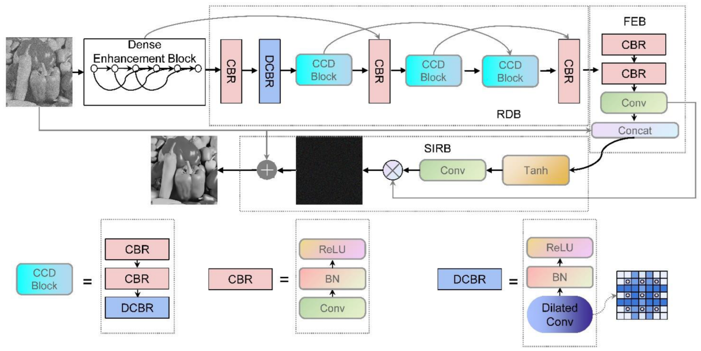
Our proposed DRFENet consists of 23 convolution layers, including 4 dilated convolution layers and 19 standard convolution layers. To alleviate the problem of gradient disappearance, we added batch normalization [36] and a rectified linear unit (ReLU) [37] to the convolutional layer. DRFENet is mainly composed of DEB, RDB, FEB, and SIRB modules, as shown in Figure 1. In DEB, we used skip connection layers to make the model learn noise information and form a hidden supervision network to review the previously learned features during each skipping continuously. The RDB module enhances the effect of the concatenated dilated convolution with skip connections, which extract noise features at different image scales. FEB plays a role in feature enhancement for RDB, which is combined with the original noise image to enhance the ability of the network to carry information. SIRB plays the same role as the attention and reconstruction blocks in ADNET to enhance the attention mechanism and reconstruction of noise. For the remainder of this section, let $X_N$ be an input noisy image. This section will show the specific flow of $X_N$ into DRFENet.

Figure 1. Architecture of proposed DRFENet network.

3.1. Dense Enhancement Block

Skip connections simplify the transmission of high-level information to enhance noise expression, improving image denoising [38]. We establish the connection between different layers and fully use the feature map to alleviate the problem of gradient disappearance. Meanwhile, this connection mode makes the transmission of features more effective, making the network easier to train. Aiming further to enhance the feature expression ability of the network, we optimized the dense block of Densenet for the image-denoising task [34].

This structure can reuse the output of each convolution layer to extract more information, but this is also its disadvantage. In the original dense block, all the features output by the convolutional layer are reused in the subsequent convolutional layer. The deep layer receives extensive useless feature information that contributes to parameter redundancy.

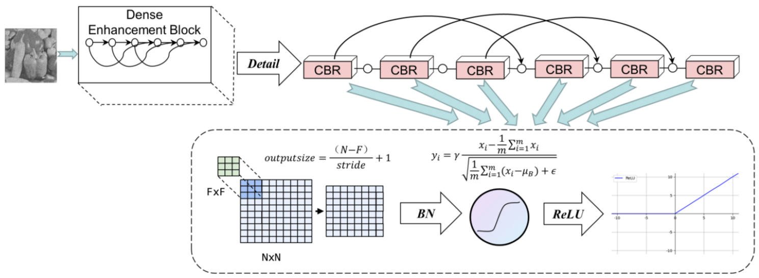
We create a new block that passes information from the first three convolutional layers to the next three layers in batches. In other words, the first three convolutional layers will share characteristic parameters with the third one that follows it. We call this strategy interval transmission. This feature reuse strategy reduces the parameter redundancy, and the deep layer distils fit feature information. DEB reduces the feature graph immediately after the skip connection so that the output feature graph of each convolution layer is maintained at 64 to avoid feature map redundancy. The last three layers of the network implicitly depth-monitor their predecessors.

The DEB Is shown in Figure 2. Connecting lines in the figure represent a skip connection. The DEB is a six-layer CBR structure. The CBR in the sixth layer can alleviate the problem of gradient explosion and gradient extinction by transmitting the output information of the first three layers to the second three layers according to interval transmission. The DEB can be expressed in Equation (1). The details of the DEB are expressed in Equation (2).

$$O_{DEB}=F_{DEB}\left(X_N\right),$$

(1)

$$\begin{gathered} O_{DEB.CBR1}=F_{CBR}\left(X_N\right) \\ {O}_{DEB.CBR2}=F_{CBR}\left(O_{DEB.CBR1}\right) \\ {O}_{DEB.CBR3}=F_{CBR}\left(O_{DEB.CBR2}\right) \\ {O}_{DEB.CBR4}=F_{CBR}\left(Cat\left(O_{DEB.CBR1},O_{DEB.CBR3}\right)\right) \\ {O}_{DEB.CBR5}=F_{CBR}\left(Cat\left(O_{DEB.CBR2},O_{DEB.CBR4}\right)\right) \\ {O}_{DEB}=F_{CBR}\left(Cat\left(O_{DEB.CBR3},O_{DEB.CBR5}\right)\right) \end{gathered}$$

(2)

where $F_{DEB}$, $O_{DEB}$, $F_{CBR}$, $Cat$, and $O_{DEB.CBR\left(1,2,3,4,5\right)}$ denote the function of the DEB, the output of the DEB, the function of CBR, the skip connection, and the CBR output for each layer, respectively.

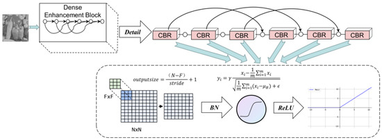
Figure 2. DEB in DRFENet.

3.2. Residual Dilated Block

The RDB consists of nine convolution layers and four dilation convolution layers. Dilation convolution layers are arranged in the 8th, 11th, 15th, and 18th layers of the overall network in DRFENet. As shown in Figure 1, a CCD block consists of two common convolutions and dilated convolution. The position of the dilated convolution and skip connections is the essence of this module. Due to the characteristics of the CNN, the convolutional layer in the first few layers of the network often represents low-level features, such as pixel-level features. In contrast, the convolutional layer in the deep layer usually represents high-level features, such as semantic features. As the network layer deepens, the extracted features become more accurate, but part of the contextual information will also disappear. Therefore, we designed a network structure combining skip connections and dilated convolution and use a progressive reuse strategy to build a network. Dilated convolution is used to capture more context information, and skip connections are used to transfer image characteristics and captured contextual information to deeper layers of the network. The skip connection in the RDB ranges from five convolution layers in the middle to four convolution layers and then to three convolution layers. It is more convenient for high-level information transmission to form an arithmetic sequence descending step-by-step. This helps for learning features of different depths, making more effective use of the feature, and strengthening the feature’s transmission of information.

Dilated convolution can obtain a larger receptive field and thus obtain more intensive data and map more context. Therefore, it is very cost-effective to take the output of dilation convolution as the input of the skip connection, since there is more information though the network structure, and parameters are unchanged. See Equation (3) for the formula of the RDB:

$$O_{RDB}=F_{RDB}\left(O_{DEB},O_{DEB}\right),$$

(3)

where $F_{RDB}$, $O_{RDB}$ express the function and the output of the RDB, respectively. As the input of the RDB, $O_{DEB}$ is passed to the next layer connected with the second dilation convolution feature map, so $O_{DEB}$ is input twice. The $O_{RDB}$ will be the input to the FEB.

3.3. Feature Enhancement Module

While sorting out the features of the RDB, as the network deepens, problems of gradient instability and network degradation follow. We take the incoming noise map as the input to make a skip connection with the FEB to obtain more global features to alleviate these problems so that DRFENet can have an overall understanding of image details. The 19th and 20th layers of the FEB are CBR structures. Then, the convolution of the 21st layer is used for dimensionality reduction, which is combined with the incoming noise map’s characteristic map. The FEB can be expressed by Equation (4), and the details of the FEB are shown in Equation (5):

$$O_{FEB.Conv}=F_{Conv}\left(F_{CBR}\left(F_{CBR}\left(O_{RDB}\right)\right)\right),$$

(4)

$$\begin{gathered} O_{FEB}=Cat\left(O_{FEB.Conv},X_N\right) \\ =F_{FEB}\left(O_{RDB},X_N\right), \end{gathered}$$

(5)

where $O_{FEB.Conv}$ and $O_{FEB}$ $O_{RDB}$ and $X_{IN}$ are the input from the upper layer and noise image. $F_{Conv}$ and $F_{FEB}$ are represented as the corresponding function.

3.4. Simultaneous Iterative Reconstruction

SIRB adopts a structure similar to ADNet [29]. AB is used in ADNet to guide the CNN training denoising model, and an attention mechanism is used to strengthen noise separation. To blend more image features and to differentiate the channel features, DRFENet employs a Tanh activation function that converges faster than Sigmoid.

A convolution of $2C\times 1\times 1\times C$ is used in the 22nd layer, where C is the number of channels passed into the noisy image. The weight obtained by using the convolution is multiplied by $O_{FEB.Conv}$ to extract more prominent noise features, which helps in generating the noise map from complex backgrounds. Finally, the RL technique is used to reconstruct the clean image by subtracting the pure noise image from the original noise image. SIRB is shown in Equation (6). The specific steps of SIRB are elaborated in Equation (7):

$$O_{SIRB}=F_{SIRB}\left(O_{FEB},O_{FEB.Conv},X_N\right),$$

(6)

$$\begin{gathered} O_{noise}=O_{FEB.Conv}\times F_{Conv}\left(F_{Tanh}\left(O_{FEB}\right)\right) \\ {O}_{SIRB}=X_N-O_{noise}, \end{gathered}$$

(7)

where $O_{noise}$ and $O_{SIRB}$ are the outputs of the noise and image denoising, respectively, and $F_{Conv}$ and $F_{FEB}$ are the corresponding function.

3.5. Loss Function

The mean absolute error (L1 loss, MAE) and the mean squared error (L2 loss, MSE) are commonly used loss functions in the field of images.

The MSE is the sum of the squares of the difference between the target variable and the predicted value, so L2 loss will capture the average feature weight and a stable solution. DRFENet uses MSE to predict the residual image. Equation (8) shows the formula for finding MSE from a clean image I and a noise image K with a given image size of m × n:

$$\mathrm{MSE}=\frac{1}{mn}{{\displaystyle \sum }}_{i=0}^{m-1}{{\displaystyle \sum }}_{j=0}^{n-1}{\left[I\left(i,j\right)-K\left(i,j\right)\right]}^2,$$

(8)

The training dataset is rendered as ${\left\{X_C, X_N\right\}}_{i=1}^N$, where $X_C$ and $X_N$ represent the clear image, noise image, and input noisy image, respectively. DRFENet is trained to create the noise mapping, and it then uses the noisy image minus the noise mapping to obtain a clean image, as shown in Equation (9). Letting y stand for the clear image, it is easy to derive Equation (10):

$$y=X_N-F_{BTBUNet}\left(X_N\right),$$

(9)

$$F_{BTBUNet}\left(X_N\right)=X_N-y,$$

(10)

where $F_{BTBUNet}\left(X_{IN}\right)$ denotes the noise mapping. In this study, the noise mapping generated in Equation (11) is used to calculate the loss function:

$$l\left(\mathsf{\Theta }\right)=\frac{1}{N}{{\displaystyle \sum }}_{n=1}^N{\left(F_{BTBUNet}\left(X_N\right)-\left(X_N-X_C\right)\right)}^2,$$

(11)

where Θ and N are the numbers of parameters and noisy image patches, respectively.

To verify the effect of MAE and MSE, we conducted a control test, as shown in Table 1.

Table 1. Average PSNR (dB) results of MSE and MAE on Set12 and BSD68 with noise levels of 15, 25, and 50.

Noise Level	Set12		BSD68
Methods	L1 Loss (MAE)	L2 Loss (MSE)	L1 Loss (MAE)	L2 Loss (MSE)
σ = 15	32.92	32.96	31.73	31.76
σ = 25	30.50	30.54	29.22	29.26
σ = 50	27.29	27.33	26.25	26.29

4. Results and Discussions

4.1. Implementation Details

This study used the Berkeley Segmentation Dataset (BSD) of size 180 × 180 [8] and 100 pristine natural images from the Waterloo Exploration Database [39] for training. We introduced three known noise levels (σ = 15, 25, and 50) into the gray image datasets for image denoising. For color image denoising, we introduced five known noise levels (σ = 15, 25, 35, 50, and 75). We set the patch size as 50 × 50 and the stride as 40.

The test set and the training set are also divided into gray images and color images. We used McMaster [40], Kodak24 [41], and CBSD68 as the test datasets of color images. McMaster and Kodak24 are 18 image sets and 24 image sets, respectively, with a size of 500 × 500. CBSD68 is 68 natural images with a size of either 481 × 321 or 321 × 481.

BSD68 and Set12 [42] were used as the test set of gray images. BSD68 is the gray version of the color test dataset CBSD68. Set12 is a natural square image with a size of 256 × 256, and there are 12 images in total.

The data used in this study do not need to be anonymous before use.

The network depth of DRFENet is 23 layers. Our initial learning rate started from 10⁻³ to train 20 epochs, then every 10epochs eps was 1/10 of the previous one and finally stopped when eps = 10⁻⁸. The batch size of the training was 128, β1 = 0.9, β2 = 0.999. Our experimental environment was all completed in Windows 10, the Python environment was 3.8, the PyTorch version was 1.7.1, and the main hardware configuration of the PC is shown in Table 2.

Table 2. Implementation details.

Device Name	Unit Type	Amount
CPU	Intel® Core™ i7-10700K Processor	1
Mainboard	ASUS PRIME Z490-P	1
GPU	Nvidia Geforce RTX 3090	1
Memory	8 GB(DDR4 3200 MHz)	4

4.2. Evaluation Indicators

To verify the effectiveness of each part of DRFENet, we used a controlled trial to test the performance of different modules of DRFENet. To improve the information exchange between the channels and broaden the receptive field of the model, we used DEB and RDB to test skip connections at different positions. We tested four configurations: the skip connection before dilated convolution, the RDB without skip connection, DRFENet without DEB, DRFENet without RDB, and the full DRFENet. We took the peak signal-to-noise ratio (PSNR) and the structural similarity (SSIM) as targets for assessing the image denoising effect.

PSNR is the most common and widely used objective measurement method to evaluate picture quality. The formula is shown in Equation (12):

$$\mathrm{PSNR}=10·{\log }_{10}\left(\frac{MA{X}_I^2}{MSE}\right),$$

(12)

where $MA{X}_I^2$ is the maximum pixel value of the image: if the pixel value is represented by K-bit binary, then $MA{X}_I=2^K-1$. The SSIM formula is based on three comparative measures between two samples: luminance, contrast, and structure, as shown in Equation (13):

$$\mathrm{SSIM}\left(\mathrm{x},\mathrm{y}\right)=\frac{\left(2{\mu }_x{\mu }_y+c_1\right)\left(2{\sigma }_{xy}+c_2\right)}{\left({\mu }_x^2+{\mu }_y^2+c_1\right)\left({\sigma }_x^2+{\sigma }_y^2+c_2\right)},$$

(13)

where x and y are two different photos, ${\mu }_x$ and ${\mu }_y$ are the mean of x and y, ${\sigma }_{xy}$ is the covariance of x and y, and ${\sigma }_x^2$ and ${\sigma }_y^2$ are the variance of x and y, respectively.

Finally, we found a more practical scheme to build the 23-layer neural network, which not only had an excellent overall denoising performance but also showed a better effect on the recovery of local features.

4.3. Experimental Results

In this chapter, we first performed ablation experiments to verify the effectiveness of each component of the model. Then, we compared the performance of DRFENet with traditional image denoising methods and different convolutional neural network models in gray datasets and color datasets, respectively. The traditional denoising method was BM3D [6]. The CNN-based methods we compared against were DnCNN [10], IRCNN [43], BRDNet [44], ECNDNet [31], and ADNet [29]. For all comparison methods, the model was derived from the code provided by the original paper or according to the original paper. We used the same dataset to train all networks to ensure fairness. Finally, in order to verify the difference between the model and other models, we used the analysis of variance (ANOVA) for statistical analysis of the proposed results.

4.3.1. Ablation Experiment

To verify the effectiveness of each module of DRFENet, the important functions in our model are separated to complete the ablation experiment: (1) Use the strategy of placing the skip connection before dilated convolution in the RDB module and converting scale after fusion. (2) Do not use skip connections to aggregate different scales in the RDB module. (3) Remove the DEB module in the shallow layer of the network. (4) Remove the attention mechanism of weight multiplication in SIRB. (5) Implement DRFENet without FEB and SIRB without multiplication of weights. (6) Remove the RDB module. (7) Complete DRFENet. In order to ensure the effectiveness of the ablation experiment, we conducted experiments in Set12 and BSD68 datasets, consisting of 12 images and 68 images, respectively. The average value of ten experiments was selected as the experimental result, and the same noise map was used to attack the images in each batch of experiments. Comparison tests are shown in Table 3. It can be seen from the results that when the skip connection is placed before dilated convolution, the strategy of transforming the scale after fusion is not as good as the progressive reuse strategy we proposed in obtaining more feature information. When long skip connections are abandoned in RDB, the communication between multiple scales is weakened, and the integrity of the network is damaged. When there is no DEB in DRFENet, a large amount of feature information is lost in the shallow layer of the network, resulting in insufficient global feature learning in the network. When the multiplication of weights is removed from the SIRB, the model loses the ability to extract more prominent noise features at the end. When DRFENet does not have the FEB, the network loses the opportunity to revisit global features at a deep level. The RDB is the backbone module in DRFENet that has the most frequent feature learning. When DRFENet does not have the RDB, the reasoning ability of DRFENet also plummets.

Table 3. Average PSNR (dB) of ablation experiment on Set12 with noise levels of 25.

Methods	Set12	BSD68
skip connection before dilated convolution	30.519211	29.253672
RDB without skip connection	30.522240	29.249066
DRFENet without DEB	30.478824	29.232598
SIRB without Multiplication of weights	30.535542	29.254584
DRFENet without FEB and SIRB without Multiplication of weights	30.497805	29.244180
DRFENet without RDB	30.266703	29.062368
DRFENet	30.545276	29.258824

4.3.2. Comparison with Other Different Models

We performed a gray image contrast experiment using three different noise levels (σ = 15, 25, and 50). Image denoising experiments were carried out in two different datasets, Set12 and BSD68, and their respective PSNR and SSIM values were given. The test results are shown in Table 4 and Table 5.

Table 4. Average PSNR (dB) of different methods on BSD68 with different noise levels of 15, 25, 50.

Methods		BM3D	TNRD	DnCNN	IRCNN	ECNDNet	ADNet	BRDNet	Ours
σ = 15	PSNR	31.08	31.42	31.72	31.57	31.72	31.73	31.72	31.76
	SSIM	0.8722	0.8826	0.8905	0.8872	0.8906	0.8909	0.8909	0.8919
σ = 25	PSNR	28.57	28.92	29.20	29.07	29.21	29.23	29.24	29.26
	SSIM	0.8017	0.8157	0.8269	0.8229	0.8274	0.8283	0.8293	0.8304
σ = 50	PSNR	25.62	25.97	26.22	26.09	26.22	26.26	26.28	26.29
	SSIM	0.6869	0.7029	0.7183	0.7110	0.7190	0.7201	0.7230	0.7230

Table 5. Average PSNR (dB) results of different methods on Set12 with noise levels of 15, 25, and 50.

Methods	PSNR													SSIM
Images	C.man	House	Peppers	Starfish	Monarch	Airplane	Parrot	Lena	Barbara	Boat	Man	Couple	Average
	Noise level σ = 15
BM3D	31.65	34.76	32.56	30.89	31.86	31.17	31.31	34.22	32.87	32.10	31.94	32.05	32.28	0.8946
DnCNN	32.58	35.02	33.31	32.08	33.16	31.66	31.96	34.62	32.60	32.52	32.41	32.49	32.87	0.9030
IRCNN	32.35	34.70	33.19	31.94	32.85	31.61	31.82	34.41	32.25	32.33	32.29	32.31	32.67	0.8992
ECNDNet	32.56	35.06	33.36	32.14	33.08	31.68	31.93	34.59	32.63	32.49	32.43	32.46	32.87	0.9028
ADNet	32.61	35.06	33.37	32.26	33.16	31.72	31.98	34.63	32.65	32.50	32.46	32.50	32.91	0.9035
BRDNet	32.64	35.17	33.35	32.21	33.19	31.76	31.90	34.62	32.52	32.49	32.44	32.48	32.90	0.9032
Ours	32.60	35.19	33.42	32.19	33.41	31.76	31.96	34.72	32.73	32.54	32.45	32.55	32.96	0.9048
	Noise level σ = 25
BM3D	29.27	32.75	30.12	28.34	29.20	28.49	28.73	32.08	30.52	29.81	29.63	29.67	29.88	0.8490
DnCNN	30.27	33.22	30.83	29.42	30.28	28.99	29.41	32.47	29.95	30.21	30.05	30.14	30.44	0.8617
IRCNN	29.93	32.87	30.77	29.15	30.05	28.98	29.31	32.32	29.64	30.08	29.97	29.90	30.25	0.8571
ECNDNet	30.23	33.31	30.94	29.37	30.25	29.13	29.41	32.48	29.96	30.25	30.07	30.11	30.46	0.8622
ADNet	30.15	33.32	31.06	29.40	30.41	29.16	29.50	32.56	30.05	30.24	30.09	30.17	30.51	0.8627
BRDNet	30.24	33.38	31.07	29.48	30.38	29.19	29.47	32.54	29.98	30.23	30.09	30.20	30.52	0.8636
Ours	30.26	33.41	31.07	29.49	29.49	29.12	29.46	32.57	30.02	30.29	30.07	30.17	30.54	0.8645
	Noise level σ = 50
BM3D	26.11	29.43	26.68	24.89	25.76	25.22	25.80	28.88	27.05	26.69	26.77	26.40	26.64	0.7600
DnCNN	27.10	30.25	27.34	25.60	26.70	25.95	26.45	29.41	26.30	27.16	27.16	26.94	27.20	0.7830
IRCNN	26.95	29.70	27.25	25.45	26.47	25.72	26.41	29.24	25.83	27.05	27.13	26.74	27.00	0.7762
ECNDNet	27.02	30.04	27.25	25.74	26.82	25.75	26.36	29.29	26.27	27.18	27.17	26.86	27.15	0.7827
ADNet	27.19	30.24	27.56	25.65	26.92	25.99	26.55	29.56	26.39	27.26	27.20	26.94	27.29	0.7871
BRDNet	27.10	30.63	27.52	25.67	26.85	25.88	26.52	29.47	26.53	27.24	27.23	27.07	27.31	0.7886
Ours	27.10	30.57	27.54	25.83	26.89	25.83	26.42	29.60	26.53	27.31	27.27	27.06	27.33	0.7892

We experimented on three different color image datasets (CBSD68, Kodak24, and McMaster) with six noise levels (σ = 15, 25, 35, 50, 75), and the corresponding PSNR is given in Table 6. The final experimental results show that the performance of our network model is better than that of other competitive algorithms.

Table 6. PSNR (dB) results of different methods on CBSD68, Kodak24, and McMaster datasets with noise levels of 15, 25, 35, 50, and 75.

Datesets	Methods	σ = 15	σ = 25	σ = 35	σ = 50	σ = 75
CBSD68	CBM3D	33.52	30.71	28.89	27.38	25.74
	FFDNet	33.80	31.18	29.57	27.96	26.24
	DnCNN	33.98	31.31	29.65	28.01	–
	IRCNN	33.86	31.16	29.50	27.86	–
	ADNet	33.99	31.31	29.66	28.04	26.34
	Ours	34.04	31.34	29.68	28.11	26.40
Kodak24	CBM3D	34.28	31.68	29.90	28.46	26.82
	FFDNet	34.55	32.11	30.56	28.99	27.25
	DnCNN	34.73	32.23	30.64	29.02	–
	IRCNN	34.56	32.03	30.43	28.81	–
	ADNet	34.76	32.26	30.68	29.10	27.40
	Ours	34.84	32.32	30.72	29.20	27.50
McMaster	CBM3D	34.06	31.66	29.92	28.51	26.79
	FFDNet	34.47	32.25	30.76	29.14	27.29
	DnCNN	34.80	32.47	30.91	29.21	–
	IRCNN	34.58	32.18	30.59	28.91	–
	ADNet	34.93	32.56	31.00	29.36	27.54
	Ours	35.04	32.66	31.07	29.51	27.69

Many experimental results show that the current mainstream image denoising algorithm can restore the image’s appearance by removing the noise. Still, this will make the image lose the sense of stereo. To better fit complex nonlinearities, the contour and background restoration of noisy images requires the model to have global perception ability and carry rich fine-grained information. Figure 3 is one of the images in the BSD68 dataset. We made a comparison diagram of the denoising effect to compare DRFENet with other denoising methods and enlarged part of the image for a clearer comparison. In Figure 4, we show a picture in CBSD68 to test the performance of DRFENet on color images. It can be seen that in Figure 4a–c, the network structure of DRFENet can not only restore the image more thoroughly, but also make the details of the picture smoother and retain a certain sense of stereo. As shown in Figure 4i, DRFENet can recover the contour of the image at a high noise level. These features are all due to DRFENet’s network construction, which combines dilated convolution to the RDB for learning subtle features. To enhance the expression of noise in DRFENet, we create a DEB that establishes the connection between different layers at the initial stage of the model. Huge feature information from DEB is passed into the RDB through the long path and fused with the model mainline before dilated convolution. A large number of shallow features are captured by dilated convolution. It is equivalent to reusing the information learned by the shallow convolution layer in the model mainline. In addition, the features learned from the model fused the input noise map in FEB, and the feature map after feature sorting was used as the input of the attention mechanism in SIRB through the Tanh activation function and a convolution layer. In other words, the product weighting feature with the previous mainline of the model has the quality of noise, which helps to strengthen the noise separation of the model.

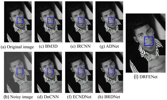
Figure 3. The image is derived from the results of different image-denoising methods of BSD68 at noise level 25. (a) Original image, (b) noisy image, (c) BM3D/PSNR = 32.88 dB/SSIM = 0.918, (d) DnCNN/PSNR = 34.13 dB/SSIM = 0.934, (e) IRCNN/PSNR = 33.64 dB/SSIM = 0.928, (f) ECNDNet/PSNR = 34.19 dB/SSIM = 0.936, (g) ADNet/PSNR = 34.21 dB/SSIM = 0.935, (h) BRDNet/PSNR = 34.22 dB/SSIM = 0.936, (i) DRFENet/PSNR = 34.29 dB/SSIM = 0.936.

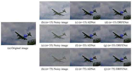
Figure 4. Noise images processed in ADNet and in DRFENet have noise levels of 15, 35, and 75, respectively. (a) Original image, (b) (σ = 15) noisy image, (c) (σ = 15) ADNet/PSNR = 42.13 dB, (d) DRFENet/PSNR = 42.25 dB, (e) (σ = 35) Noisy image, (f) (σ = 35) ADNet/PSNR = 38.44 dB, (g) DRFENet/PSNR = 38.46 dB, (h) (σ = 75) Noisy image, (i) (σ = 75) ADNet/PSNR = 34.66 dB, (j) DRFENet/PSNR = 34.92 dB.

The experimental results show that DRFENet has strong robustness and leads in both PSNR and SSIM.

4.3.3. Statistical Analysis

To further verify the robustness of the algorithm, we set up 100 experiments with different noise distributions to test the model, in which each group of experiments had the same noise graph, and we used the standard deviation and mean value to verify the stability and denoising performance of the algorithm, respectively. As shown in Table 7, the mean values and standard deviations of different models with a noise intensity of 15, 25, and 50 are respectively shown. It can be clearly seen that the standard deviation of DRFENet is generally low, which indicates that the algorithm performance is improved while maintaining high algorithm stability.

Table 7. The average PSNR(dB) results of 100 experiments and the standard deviations between each result were obtained from different methods in the Set12 dataset with noise level of 25.

Methods		DnCNN	IRCNN	ECNDNet	ADNet	BRDNet	Ours
σ = 15	Mean	32.88	32.66	32.88	32.89	32.87	32.95
	Std	0.000120	0.000122	0.000129	0.000116	0.000135	0.000119
σ = 25	Mean	30.45	30.23	30.45	30.48	30.49	30.53
	Std	0.000153	0.00018	0.000176	0.000214	0.000156	0.000175
σ = 50	Mean	27.20	26.97	27.13	27.26	27.28	27.32
	Std	0.000402	0.000362	0.000435	0.000341	0.000406	0.000387

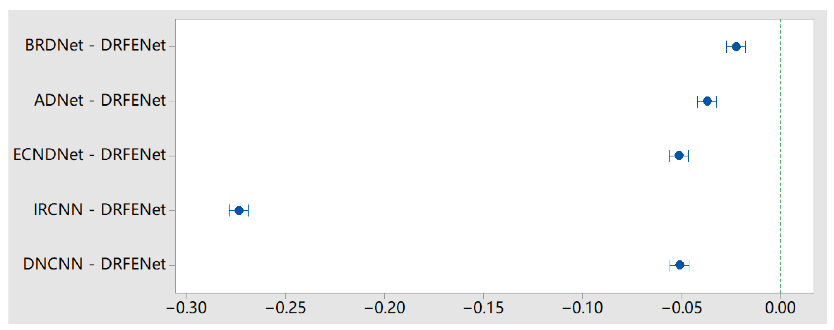
We also used the analysis of variance (ANOVA) to test the significance of the difference in means between the models. When the significance level α = 0.05, the ANOVA showed that the significance (P value) was less than 0.001 when the noise intensity was 15, 25, and 50, indicating a significant difference between DRFENet and other algorithms. The 95% confidence interval showed no overlap in the PSNR value of the noise reduction performance under the same noise intensity. This indicates that DRFENet has an advantage in any noise distribution environment.

The Dunnett t-test formula is shown in Equations (14) and (15). The Dunnett t-test formula was used to test the difference between the experimental group and the control group.

$$S_w^2=MSE\left(\frac{1}{n_i}+\frac{1}{n_0}\right)$$

(14)

$$Dunnett‘t=\frac{{\overline{X}}_i-{\overline{X}}_0}{S_w}$$

(15)

where $n_i$ represents the data volume of group i, $n_0$ represents the data volume of the control group, ${\overline{X}}_i$ represents the mean value of group i, ${\overline{X}}_0$ represents the mean value of the control group, and MSE represents the mean square error.

We compared DRFENet as a control group with the other five models. According to the Dunnett t-test, none of the horizontal mean values include 0 value, and DRFENet is significantly different from the mean values of other models. The Dunnett t-test and 95% confidence interval at a noise level of 25 are shown in Figure 5.

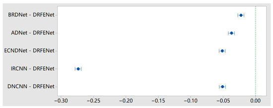
Figure 5. Dunnett t-test and 95% confidence interval at noise level of 25 in the Set12 dataset.

5. Conclusions

This paper proposes a new network structure, DRFENet, for image denoising. To improve the global perception ability of the model and more fine-grained features, we constructed DRFENet based on two proposed strategies: an interval transmission strategy and a combination strategy of concatenated dilated convolution [15] and skip connection. Four modules—DEB, RDB, FEB, and SIRB—are used for DRFENet. In the DEB, a short-range skip connection is proposed to enhance information transmission. In the RDB, a progressive skip connection is proposed to improve the effect of dilated convolution. DRFENet better reproduced local details and made a more realistic global restoration. An ablation experiment and a comparison experiment of two sets of gray images and three sets of color images showed the superiority and robustness of DRFENet, and the denoising effect of our network model algorithm was better than that of other competitive algorithms. DRFENet can restore the details of images with a high noise level, which meets the practical demands in different intelligent applications, such as mobile devices and real-time image denoising systems. In the future, we will explore integrating the proposed method into other fields.

References

- Waldspurger, I. Wavelet transform modulus: Phase retrieval and scattering. In Journées Équations Aux Dérivées Partielles; Cedram: Roscoff, France, 2017; pp. 1–10. [Google Scholar]
- Ruikar, S.; Doye, D.D. Image denoising using wavelet transform. In Proceedings of the 2010 International Conference on Mechanical and Electrical Technolog, Singapore, 10–12 September 2010; pp. 509–515. [Google Scholar]
- Buades, A.; Coll, B.; Morel, J.M. A non-local algorithm for image denoising. In Proceedings of the 2005 IEEE Computer Society Conference on Computer Vision and Pattern Recognition, San Diego, CA, USA, 20–25 June 2005; pp. 60–65. [Google Scholar]
- Dauwe, A.; Goossens, B.; Luong, H.Q.; Philips, W. A fast non-local image denoising algorithm. In Image Processing: Algorithms and Systems VI; SPIE: Bellingham, WA, USA, 2008; Volume 6812, pp. 324–331. [Google Scholar]
- Wang, J.; Guo, Y.; Ying, Y.; Liu, Y.; Peng, Q. Fast non-local algorithm for image denoising. In Proceedings of the 2006 International Conference on Image Processing, Atlanta, GA, USA, 8–11 October 2006; pp. 1429–1432. [Google Scholar]
- Dabov, K.; Foi, A.; Katkovnik, V.; Egiazarian, K. Image denoising by sparse 3-D transform-domain collaborative filtering. In IEEE Transactions on Image Processing; IEEE: Piscataway, NJ, USA, 2007; Volume 16, pp. 2080–2095. [Google Scholar]
- Dabov, K.; Foi, A.; Katkovnik, V.; Egiazarian, K. Color image denoising via sparse 3D collaborative filtering with grouping constraint in luminance-chrominance space. In 2007 IEEE International Conference on Image Processing; IEEE: Piscataway, NJ, USA, 2007; Volume 1, pp. I-313–I-316. [Google Scholar]
- Chen, Y.; Pock, T. Trainable nonlinear reaction diffusion: A flexible framework for fast and effective image restoration. In IEEE Transactions on Pattern Analysis and Machine Intelligence; IEEE: Piscataway, NJ, USA, 2016; Volume 39, pp. 1256–1272. [Google Scholar]
- Burger, H.C.; Schuler, C.J.; Harmeling, S. Image denoising: Can plain neural networks compete with BM3D? In Proceedings of the 2012 IEEE Conference on Computer Vision and Pattern Recognition, Providence, RI, USA, 16–21 June 2012; pp. 2392–2399. [Google Scholar]
- Zhang, K.; Zuo, W.; Chen, Y.; Meng, D.; Zhang, L. Beyond a gaussian denoiser: Residual learning of deep cnn for image denoising. In IEEE Transactions on Image Processing; IEEE: Piscataway, NJ, USA, 2017; Volume 26, pp. 3142–3155. [Google Scholar]
- Zhang, K.; Zuo, W.; Zhang, L. FFDNet: Toward a fast and flexible solution for CNN-based image denoising. In IEEE Transactions on Image Processing; IEEE: Piscataway, NJ, USA, 2018; Volume 27, pp. 4608–4622. [Google Scholar]
- Guo, S.; Yan, Z.; Zhang, K.; Zuo, W.; Zhang, L. Toward convolutional blind denoising of real photographs. In Proceedings of the IEEE/CVF Conference on Computer Vision and Pattern Recognition, Long Beach, CA, USA, 15–20 June 2019; pp. 1712–1722. [Google Scholar]
- Anwar, S.; Barnes, N. Real image denoising with feature attention. In Proceedings of the IEEE/CVF International Conference on Computer Vision, Long Beach, CA, USA, 15–20 June 2019; pp. 3155–3164. [Google Scholar]
- Li, Y.; Chen, X.; Zhu, Z.; Xie, L.; Huang, G.; Du, D.; Wang, X. Attentionguided unified network for panoptic segmentation. In Proceedings of the IEEE Conference on Computer Vision and Pattern Recognition, Long Beach, CA, USA, 15–20 June 2019; pp. 7026–7035. [Google Scholar]
- Yu, F.; Koltun, V. Multi-scale context aggregation by dilated convolutions. In Proceedings of the Computer Vision and Pattern Recognition, Boston, MA, USA, 7–12 June 2015. [Google Scholar]
- Jin, X.; Zhang, J.; Kong, J.; Bai, Y.; Su, T. A Reversible Automatic Selection Normalization (RASN) Deep Network for Predicting in the Smart Agriculture System. Agronomy 2022, 12, 591. [Google Scholar] [CrossRef]
- Jin, X.-B.; Gong, W.-T.; Kong, J.-L.; Bai, Y.-T.; Su, T.-L. A Variational Bayesian Deep Network with Data Self-Screening Layer for Massive Time-Series Data Forecasting. Entropy 2022, 24, 335. [Google Scholar] [CrossRef] [PubMed]
- Kawar, B.; Elad, M.; Ermon, S.; Song, J. Denoising diffusion restoration models. arXiv 2022, arXiv:2201.11793. [Google Scholar]
- Li, H.; Yang, Y.; Chang, M.; Feng, H.; Xu, Z.; Li, Q.; Chen, Y. Srdiff: Single image super-resolution with diffusion probabilistic models. Neurocomputing 2022, 479, 47–59. [Google Scholar] [CrossRef]
- Benton, J.; Shi, Y.; De Bortoli, V.; Deligiannidis, G.; Doucet, A. From Denoising Diffusions to Denoising Markov Models. arXiv 2022, arXiv:2211.03595. [Google Scholar]
- Dosovitskiy, A.; Beyer, L.; Kolesnikov, A.; Weissenborn, D.; Zhai, X.; Unterthiner, T.; Dehghani, M.; Minderer, M.; Heigold, G.; Gelly, A.; et al. An image is worth 16 × 16 words: Transformers for image recognition at scale. arXiv 2020, arXiv:2010.11929. [Google Scholar]
- Liu, Z.; Lin, Y.; Cao, Y.; Hu, H.; Wei, Y.; Zhang, Z.; Lin, S.; Guo, B. Swin transformer: Hierarchical vision transformer using shifted windows. In Proceedings of the IEEE/CVF International Conference on Computer Vision, Montreal, QC, Canada, 10–17 October 2021; pp. 10012–10022. [Google Scholar]
- Xu, K.; Li, W.; Wang, X.; Wang, X.; Yan, K.; Hu, X.; Dong, X. CUR Transformer: A Convolutional Unbiased Regional Transformer for Image Denoising. ACM Trans. Multimed. Comput. Commun. Appl. (TOMM) 2022. [Google Scholar] [CrossRef]
- Jin, X.-B.; Gong, W.-T.; Kong, J.-L.; Bai, Y.-T.; Su, T.-L. PFVAE: A Planar Flow-Based Variational Auto-Encoder Prediction Model for Time Series Data. Mathematics 2022, 10, 610. [Google Scholar] [CrossRef]
- Kong, J.L.; Wang, H.X.; Yang, C.C.; Jin, X.; Zuo, M.; Zhang, X. A Spatial Feature-Enhanced Attention Neural Network with High-Order Pooling Representation for Application in Pest and Disease Recognition. Agriculture 2022, 12, 500. [Google Scholar] [CrossRef]
- Kong, J.; Yang, C.; Lin, S.; Ma, K.; Zhu, Q. A Graph-related high-order neural network architecture via feature aggregation enhancement for identify application of diseases and pests. Comput. Intell. Neurosci. 2022, 2022, 4391491. [Google Scholar] [CrossRef] [PubMed]
- Kong, J.; Yang, C.; Wang, J.; Wang, X.; Zuo, M.; Jin, X.; Lin, S. Deep-stacking network approach by multisource data mining for hazardous risk identification in IoT-based intelligent food management systems. Comput. Intell. Neurosci. 2021, 2021, 16. [Google Scholar] [CrossRef] [PubMed]
- Zhang, Q.; Xiao, J.; Tian, C.; Lin, J.C.-W.; Zhang, S. A robust deformed convolutional neural network (CNN) for image denoising. CAAI Trans. Intell. Technol. 2022, 1–12. [Google Scholar] [CrossRef]
- Tian, C.; Xu, Y.; Li, Z.; Zuo, W.; Fei, L.; Liu, H. Attention-guided CNN for image denoising. Neural Netw. 2020, 124, 117–129. [Google Scholar] [CrossRef] [PubMed]
- Long, J.; Shelhamer, E.; Darrell, T. Fully convolutional networks for semantic segmentation. In Proceedings of the IEEE Conference on Computer Vision and Pattern Recognition, Boston, MA, USA, 7–12 June 2015; pp. 3431–3440. [Google Scholar]
- Tian, C.; Xu, Y.; Fei, L.; Wang, J.; Wen, J.; Luo, N. Enhanced CNN for image denoising. CAAI Trans. Intell. Technol. 2019, 4, 17–23. [Google Scholar] [CrossRef]
- Wang, T.; Sun, M.; Hu, K. Dilated deep residual network for image denoising. In Proceedings of the 2017 IEEE 29th International Conference on Tools with Artificial Intelligence, Boston, MA, USA, 6–8 November 2017; pp. 1272–1279. [Google Scholar]
- Ren, H.; El-Khamy, M.; Lee, J. Dn-resnet: Efficient deep residual network for image denoising. In Proceedings of the Asian Conference on Computer Vision, Perth, Australia, 4–6 December 2018; pp. 215–230. [Google Scholar]
- Huang, G.; Liu, Z.; Van Der Maaten, L.; Weinberger, K.Q. Densely connected convolutional networks. In Proceedings of the IEEE Conference on Computer Vision and Pattern Recognition, Honolulu, HI, USA, 21–26 July 2017; pp. 4700–4708. [Google Scholar]
- Ronneberger, O.; Fischer, P.; Brox, T. U-net: Convolutional networks for biomedical image segmentation. In Proceedings of the International Conference on Medical Image Computing and Computer-Assisted Intervention, Munich, Germany, 5–9 October 2015; Springer: Berlin/Heidelberg, Germany, 2015; pp. 234–241. [Google Scholar]
- Ioffe, S.; Szegedy, C. Batch normalization: Accelerating deep network training by reducing internal covariate shift. In Proceedings of the International Conference on Machine Learning, Lille, France, 6–11 July 2015; pp. 448–456. [Google Scholar]
- Glorot, X.; Bordes, A.; Bengio, Y. Deep sparse rectifier neural networks. In Proceedings of the Fourteenth International Conference on Artificial Intelligence and Statistics, Fort Lauderdale, FL, USA, 11–13 April 2011; pp. 315–323. [Google Scholar]
- Anwar, S.; Huynh, C.P.; Porikli, F. Identity Enhanced Residual Image Denoising. In Proceedings of the IEEE/CVF Conference on Computer Vision and Pattern Recognition Workshops, Seattle, WA, USA, 14–19 June 2020; pp. 520–521. [Google Scholar]
- Ma, K.; Duanmu, Z.; Wu, Q.; Wang, Z.; Yong, H.; Li, H.; Zhang, L. Waterloo exploration database: New challenges for image quality assessment models. In IEEE Transactions on Image Processing; IEEE: Piscataway, NJ, USA, 2016; Volume 26, pp. 1004–1016. [Google Scholar]
- Zhang, L.; Wu, X.; Buades, A.; Li, X. Color demosaicking by local directional interpolation and nonlocal adaptive thresholding. J. Electron. Imaging 2011, 20, 023016. [Google Scholar]
- Franzen, R. Kodak Lossless True Color Image. 2010. Available online: http://r0k.us/graphics/kodak/ (accessed on 18 January 2022).
- Roth, S.; Black, M.J. Fields of experts. Int. J. Comput. Vis. 2009, 82, 205. [Google Scholar] [CrossRef]
- Zhang, K.; Zuo, W.; Gu, S.; Zhang, L. Learning deep CNN denoiser prior for image restoration. In Proceedings of the IEEE Conference on Computer Vision and Pattern Recognition, Honolulu, HI, USA, 21–26 July 2017; pp. 3929–3938. [Google Scholar]
- Tian, C.; Xu, Y.; Zuo, W. Image denoising using deep CNN with batch renormalization. Neural Netw. 2020, 121, 461–473. [Google Scholar] [CrossRef] [PubMed]
Disclaimer/Publisher’s Note: The statements, opinions and data contained in all publications are solely those of the individual author(s) and contributor(s) and not of MDPI and/or the editor(s). MDPI and/or the editor(s) disclaim responsibility for any injury to people or property resulting from any ideas, methods, instructions or products referred to in the content. |
© 2022 by the authors. Licensee MDPI, Basel, Switzerland. This article is an open access article distributed under the terms and conditions of the Creative Commons Attribution (CC BY) license (https://creativecommons.org/licenses/by/4.0/).