Article

The Importance of Context Awareness in Acoustics-Based Automated Beehive Monitoring

1
INRS-EMT, University of Quebec, 800 Rue de la Gauchetiere Ouest, Montreal, QC H5A 1K6, Canada
2
Nectar Technologies Inc., 302-6250 Rue Hutchison, Montreal, QC H2V 4C5, Canada
3
Biology Department, Faculty of Science and Engineering, Laval University, 2325 Rue de l’Universite, Quebec, QC G1V 0A6, Canada
*
Author to whom correspondence should be addressed.
Appl. Sci. 2023, 13(1), 195; https://doi.org/10.3390/app13010195
Submission received: 27 November 2022 / Revised: 16 December 2022 / Accepted: 18 December 2022 / Published: 23 December 2022

Abstract

:
The vital role of honeybees in pollination and their high rate of mortality in the last decade have raised concern among beekeepers and researchers alike. As such, robust and remote sensing of beehives has emerged as a potential tool to help monitor the health of honeybees. Over the last decade, several monitoring systems have been proposed, including those based on in-hive acoustics. Despite its popularity, existing audio-based systems do not take context into account (e.g., environmental noise factors), and thus the performance may be severely hampered when deployed. In this paper, we investigate the effect that three different environmental noise factors (i.e., nearby train rail squealing, beekeeper speech, and rain noise) can have on three acoustic features (i.e., spectrogram, mel frequency cepstral coefficients, and discrete wavelet coefficients) used in existing automated beehive monitoring systems. To this end, audio data were collected continuously over a period of three months (August, September, and October) in 2021 from 11 urban beehives located in downtown Montréal, Québec, Canada. A system based on these features and a convolutional neural network was developed to predict beehive strength, an indicator of the size of the colony. Results show the negative impact that environmental factors can have across all tested features, resulting in an increase of up to 355% in mean absolute prediction error when heavy rain was present.

1. Introduction

Honeybees (Apis mellifera) are one of the most commercially important insects, not only because of their hive products, but also because of their pollination activity, which helps cultivation and biodiversity [1]. To ensure their health and well-being, beehive monitoring has been performed manually by beekeepers for many years. During such inspections, beekeepers visually examine colony activity and note the presence of pathogens/parasites, queen reproduction, colony worker and brood populations, and the amount of food stored. These inspections are typically performed every two weeks during the spring and summer months and are labor-intensive and time consuming for the beekeepers, as well as disruptive for the colonies.
More recently, with advances in sensing hardware, cloud computing, and machine learning tools, automated beehive monitoring tools have emerged to overcome these limitations, thus creating the field of precision beekeeping [2]. For example, systems based on beehive acoustics [3,4,5,6], hive weight [7,8,9], internal temperature [10,11], and humidity [11], as well as CO2 monitors [11] or multisensor approaches [7,8,11], have been introduced.
The weight of a beehive can be used as an indicator of honey production and bee population size, with colony weight changes being reported throughout the day. For example, weight have been reported to decrease during the night and early morning due to nectar consumption, while it increases with foraging activity during the daytime [12]. The authors in [9] monitored the weight of four colonies and showed that the average weight indicates the amount of stored food (during nectar flow), while the changes could be related to the daily consumption of food. Moreover, swarming activity can be tracked based on the weight change of the hive resulting in a sharp decrease.
Temperature stability and regulation in a beehive, in turn, can indicate the colony’s adaptive response and health state. It has been found that while the internal temperature affects the health of the bees and brood, the productivity of the hive is also strongly affected by internal hive conditions [13]. Proper thermoregulation inside the hive, for example, can help decrease mortality rates and increase honey production by reducing the internal consumption [14,15]. Moreover, it has been found that a rise in temperature (from 34 °C–35 °C to 37 °C–38 °C) could be a signature of swarming [16].
Relative humidity (RH) is another important factor for larvae growth, colony development, and bee behavior, where changes in water transportation and larvae feeding have been reported as a function of ambient humidity, hive temperature, and nectar moisture [17]. The authors in [18] used temperature and humidity sensors to monitor ambient conditions, as well as conditions within the breeding comb and the nectar areas. Their results showed that the humidity of the breeding comb was the highest (about 40% RH) and had less daily fluctuation.
Moreover, it is well known that bees communicate within the colony using vibration and acoustic signals [19] generated via the movement of their body, wings, and muscle contractions [20]. For example, specific sounds are generated during mite attacks, by failing queens [21], and during swarming [22,23]. To this end, the acoustic monitoring of beehives has emerged and is gaining popularity. In a recent literature review of beehive acoustics monitoring [24], several systems were reported showcasing tools for (i) bee activity detection [4,25,26,27], (ii) beehive strength monitoring [28], (iii) queen absence detection [3,5,29,30,31], (iv) swarming detection [22,23,32,33,34], (v) pathogen or parasite infestation detection [35], (vi) detection of environmental pollutants and chemicals [36,37,38,39], and (vii) measuring of honeybee reaction to smoke [40], as well as overall beehive monitoring (e.g., identifying normal and abnormal hive, swarming duration, bee activity time) [41,42]. From a geographical perspective, most contributions have come from the USA, UK, Japan, Slovenia, and Italy. From partially tropical countries (e.g., Mexico), experiments have mostly focused on the detection of the queen bee in Apis mellifera carnica hives [43,44]. For a more detailed overview, the interested reader is referred to [24].
One great benefit of acoustic beehive monitoring is the potential for real-time continuous monitoring, which may enable the detection of certain critical and rare events, such as queen piping [45,46]. Continuous beehive monitoring may also enable new insights into increased mortality rates observed over the last decade [47,48,49,50,51,52], which has been hypothesized to be linked to multiple stressors [53,54].
Despite the burgeoning of acoustics-based beehive monitoring applications, as the recent review in [24] showed, existing tools rely on conventional audio features that have been developed for speech processing, namely root mean square power (RMS), mel frequency cepstral coefficients (MFCCs) [55], spectrogram, and features based on the discrete wavelet transform (DWT). It is widely known within the audio processing community, however, that such parameters can be extremely sensitive to environmental factors, such as ambient noise and background speakers. As such, noise suppression and/or characterization of the background noise (known as context-awareness) are needed for the development of accurate and replicable systems (e.g., [56,57]). This will be particularly crucial for urban hives, which are on the rise [58], where loud and various urban sounds interfere with the internal hive sound recordings.
In fact, while most published studies have shown the benefits of using the acoustic signal for hive health monitoring, the majority have relied on data collected over a short period of time (e.g., 24 h), usually in the months of June and July, when rain is possible, or were collected in remote regions in the countryside; thus, they may not have been exposed to certain environmental factors known to be detrimental to the quality of audio recordings. As such, it is not clear what the impact of such events is on audio-based precision beekeeping. This paper aims to fill this gap. Acoustic data were recorded from 11 urban beehives (one was intentionally left empty) during a three-month period. The effects of three environmental factors (rain, urban sounds, and beekeeper speech) were explored on the three most popular audio features described above. To quantitatively measure the impact of such factors on system performance, results for a beehive strength prediction model are reported and drops in accuracy were measured, to validate the claim that context awareness is crucial for automated beehive monitoring systems.

2. Materials and Methods

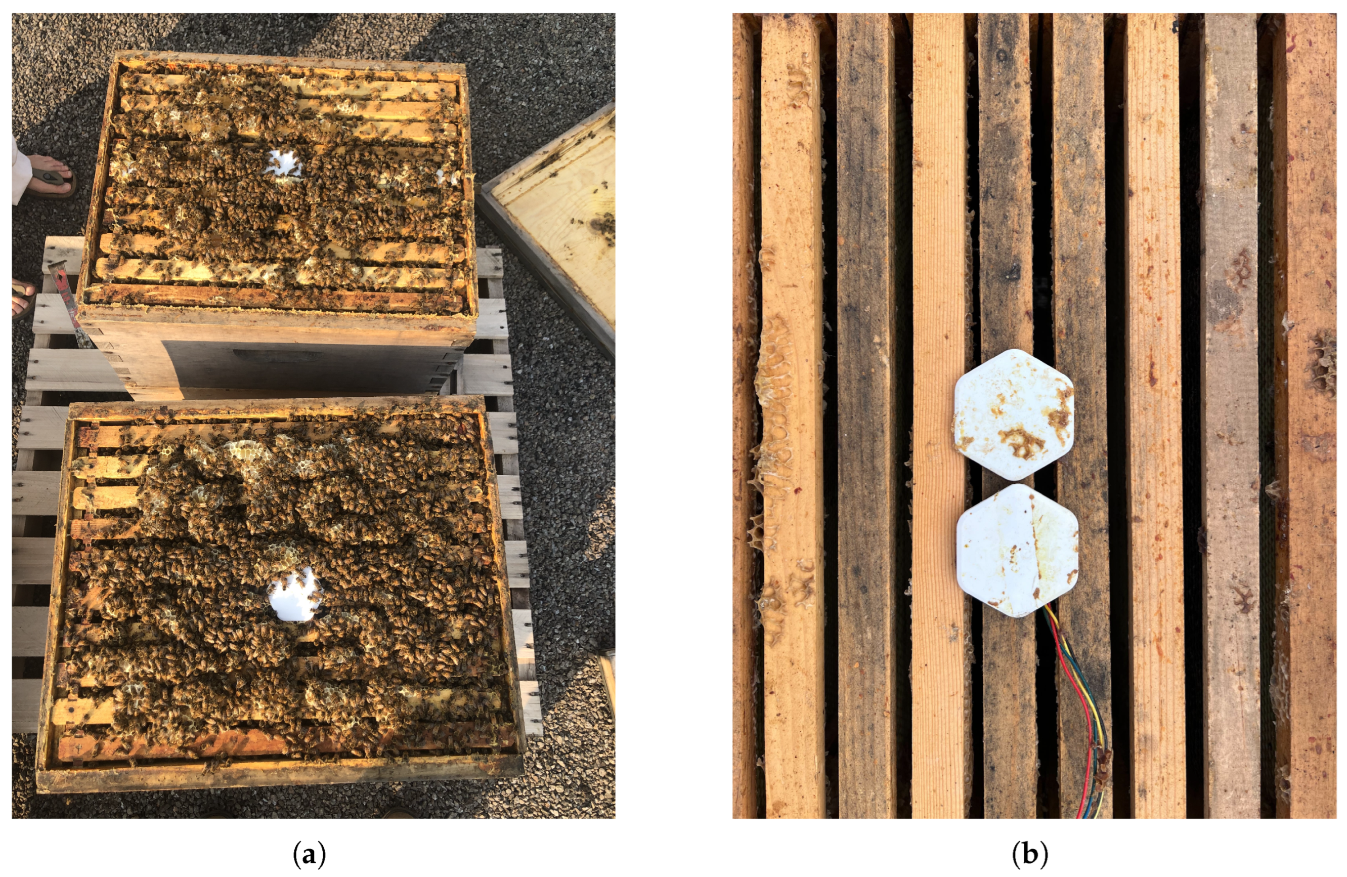
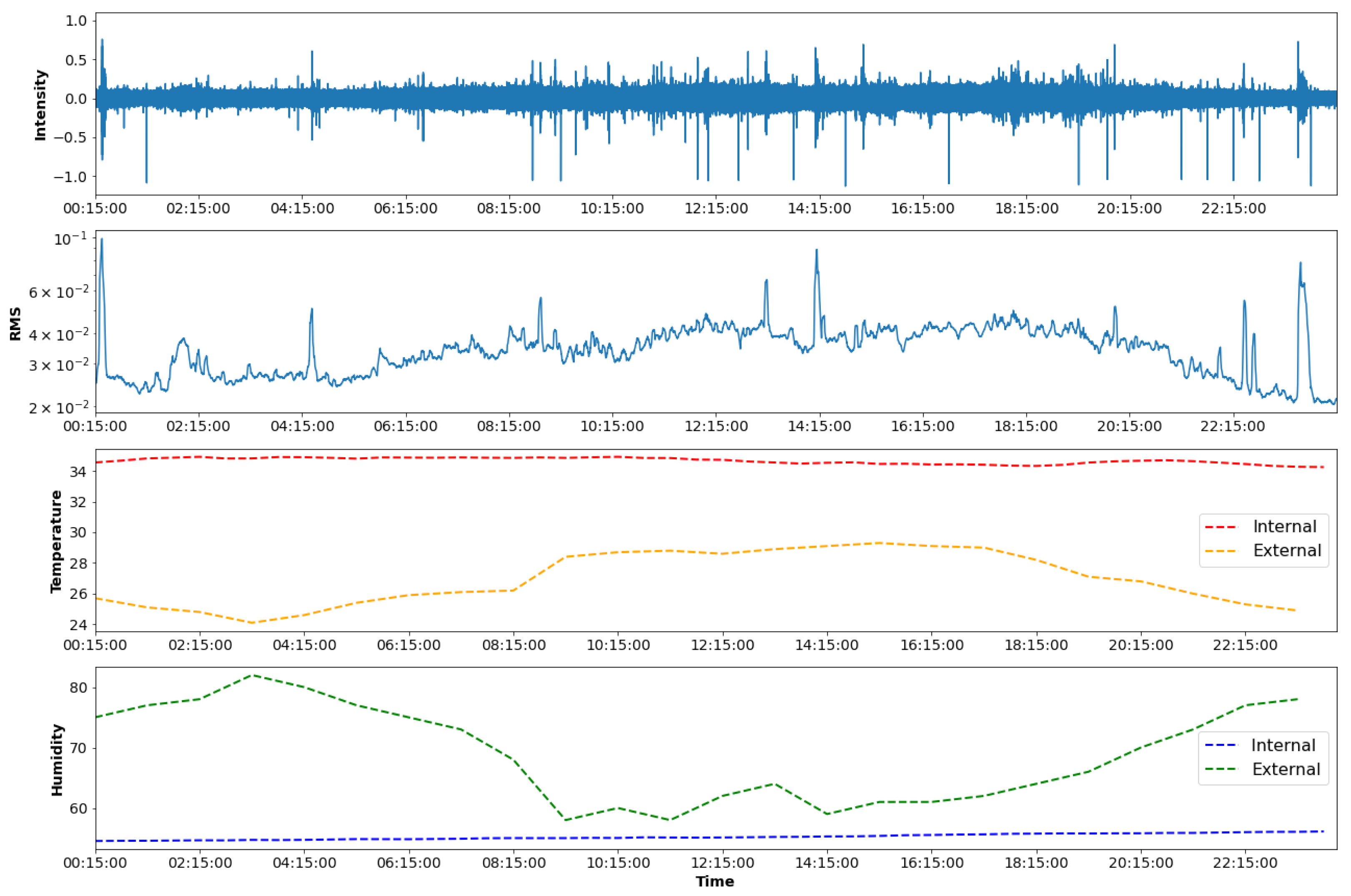
2.1. Data Acquisition

In this study, 10 beehives and 1 empty hive were monitored continuously over a three-month period on a rooftop apiary located in downtown Montréal, Québec (Canada). These hives were placed on wooden pallets (two hives per pallet) in a row facing southeast, with the empty hive placed by itself. This location facilitated ease of access to a power supply from a wall outlet on the outside of the building. Each hive comprised one brood chamber and one or two honey supers using 10-frame standard Langstroth boxes (with a maximum of three boxes), with a multimodal sensor located on top of the center frame of the bottom brood box to record the internal hive temperature and humidity (Beecon, Nectar Technologies Inc, Canada [59]), as shown in Figure 1a. and also a microphone beside that, as shown in Figure 1b. All hives came from four frame nucs that were purchased and installed in May 2021.
The nectar apiculturalists did not equalize the hive populations in order to collect data on a variety of population sizes, as the prediction of beehive strength (a correlate of population size) was one of the main goals. At the beginning of the experiment, each hive contained a different number of (full) frames of bees with a minimum of six frames of bees for a beehive with one brood box, and a maximum of 20 frames of bees for a beehive with one brood box and one honey super. As the colony populations increased, additional honey supers were added. Therefore, in our apiary, the maximum number of boxes and frames of bees were 3 and 30, respectively. Data were recorded continuously over the months of August, September, and October, 2021. The multi-modal data comprise the average temperature and humidity readings every 15 min, and a 15-min audio segment every 30 min, with a sampling rate of 48 kHz. Every two weeks, the hives were manually inspected to measure the strength of the hives (i.e., the number of frames of bees covered by least 70% [60]), to verify the presence of a laying queen, as well as to report any additional observations related to the colony activity.
Moreover, local external temperatures, humidity, and rainfall amounts levels were obtained from the Environment and Climate Change Canada website (https://climate.weather.gc.ca/, accessed on 1 June 2022.). A representative example of a 24 h snapshot of the changes in internal/external temperature and humidity levels, as well as the audio intensity and root mean square (RMS) value, is shown in Figure 2. The plots are for a strong and healthy colony in August with one brood chamber and two honey supers with a total of 30 frames of bees (covered with at least 70% of bees). As can be seen, audio power increases during the day, especially during periods in which external temperatures were increasing and external humidity levels decreasing, thus suggesting increased foraging activity and thermohygrometric regulation of the colony.

2.2. Acoustic Feature Extraction

In this section, we describe the four features that have been commonly reported to be used for audio-based precision beekeeping, namely RMS, spectrogram, MFCCs and DWT. Moreover, in Section 4, we describe the modulation spectrogram that we used. Before feature extraction, audio recordings were resampled from 48 kHz to 2048 Hz, as the literature suggests that the majority of the bee sounds are produced below 1000 Hz [24].

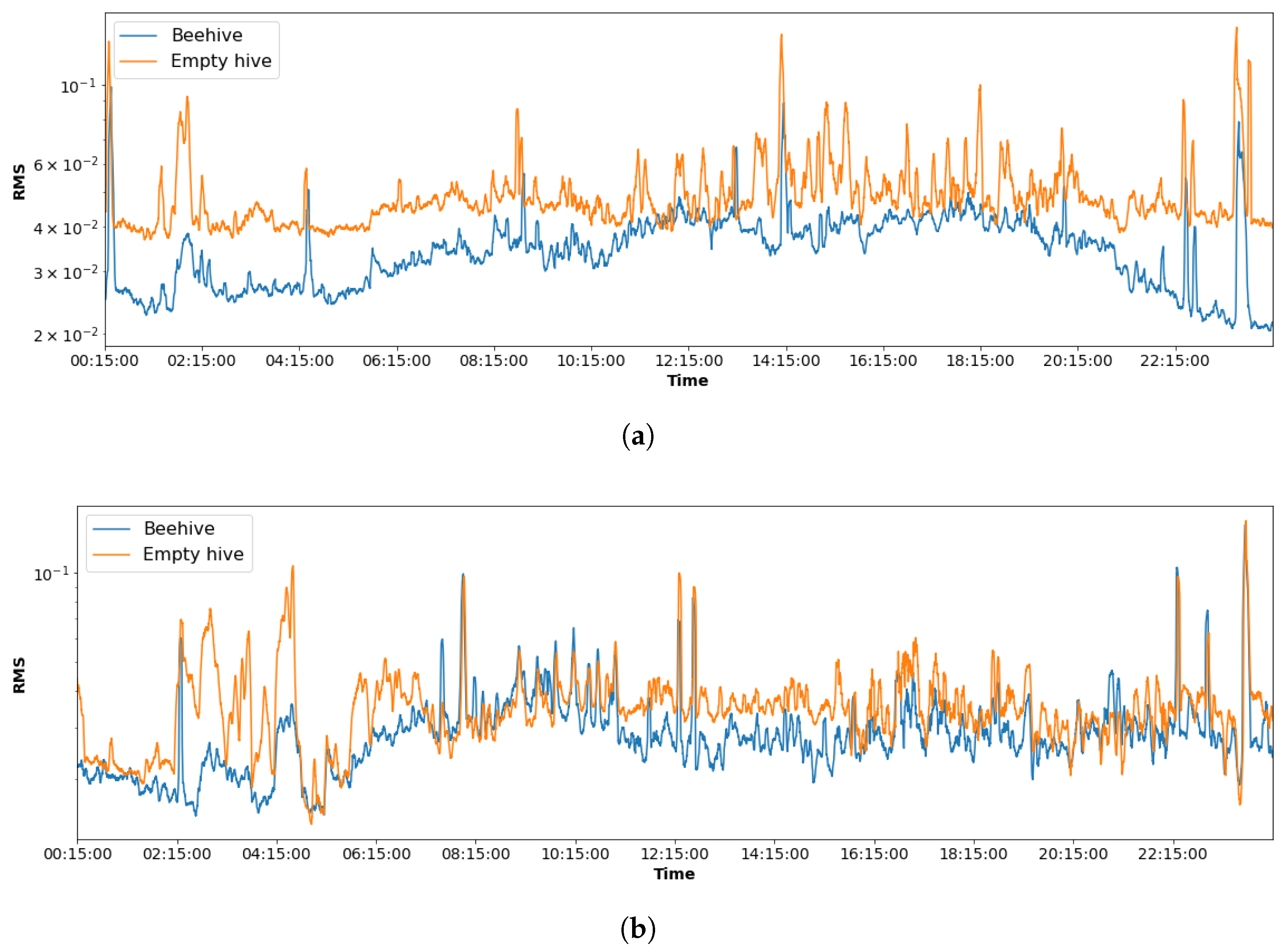
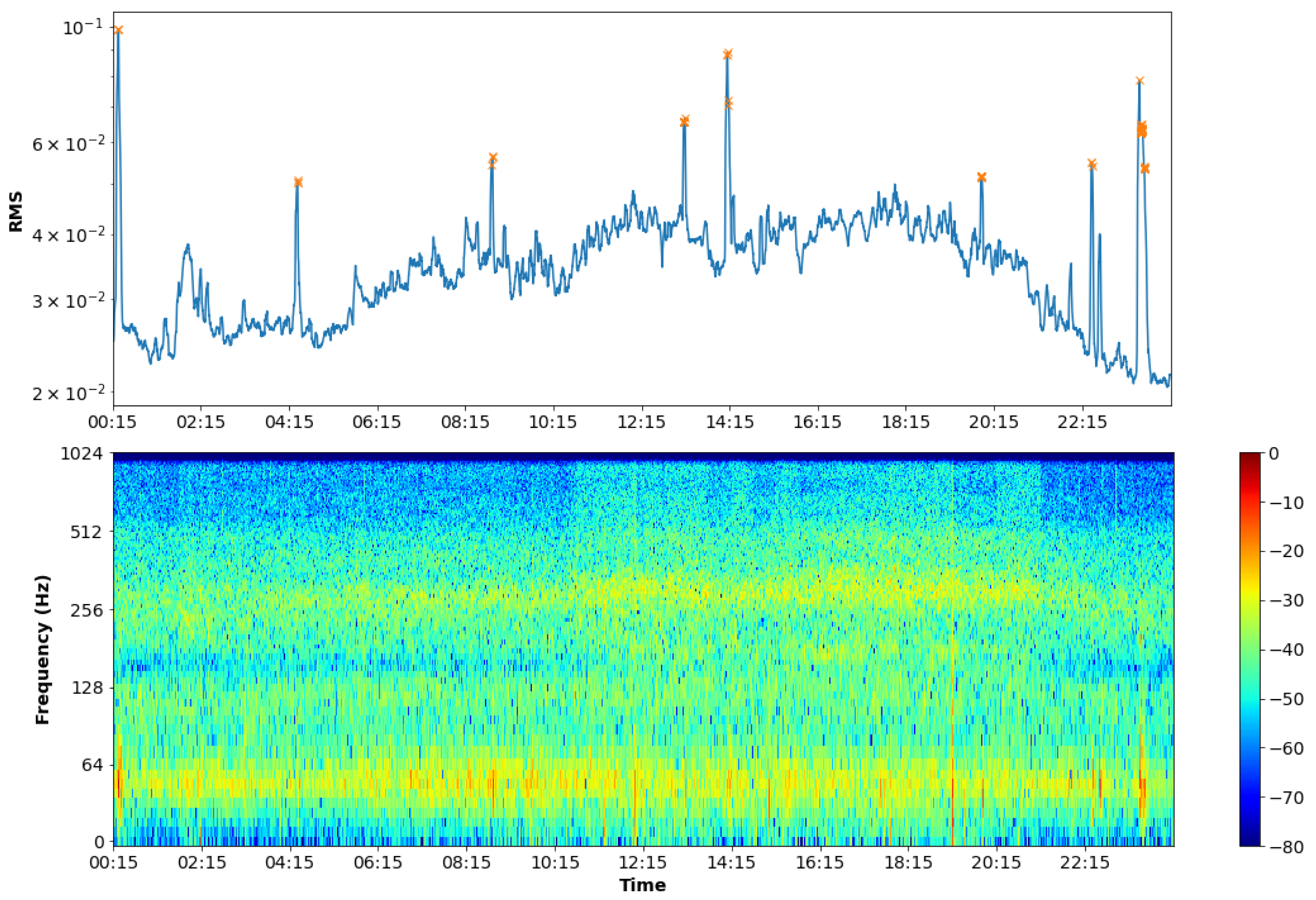
2.2.1. Root Mean Square Power
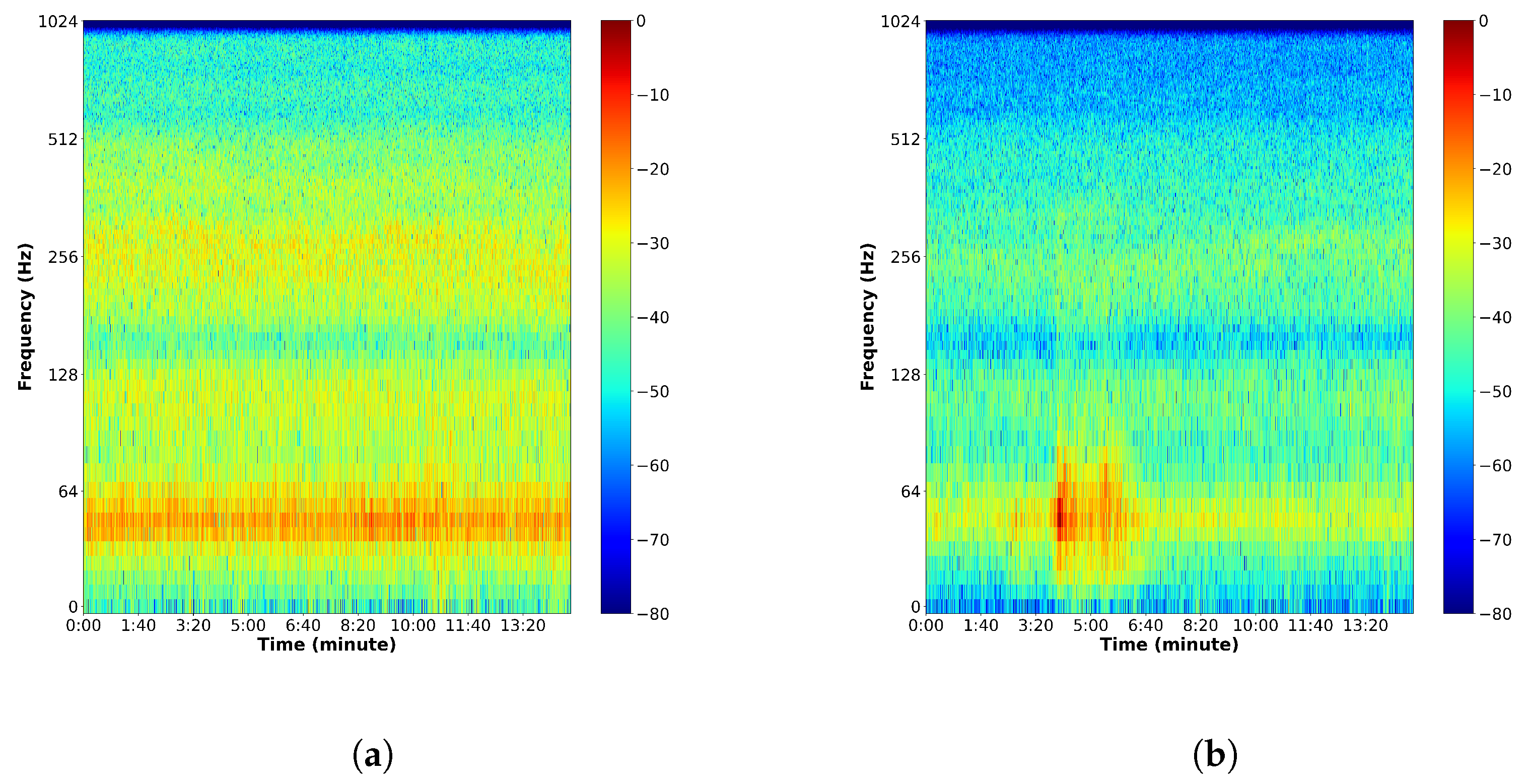
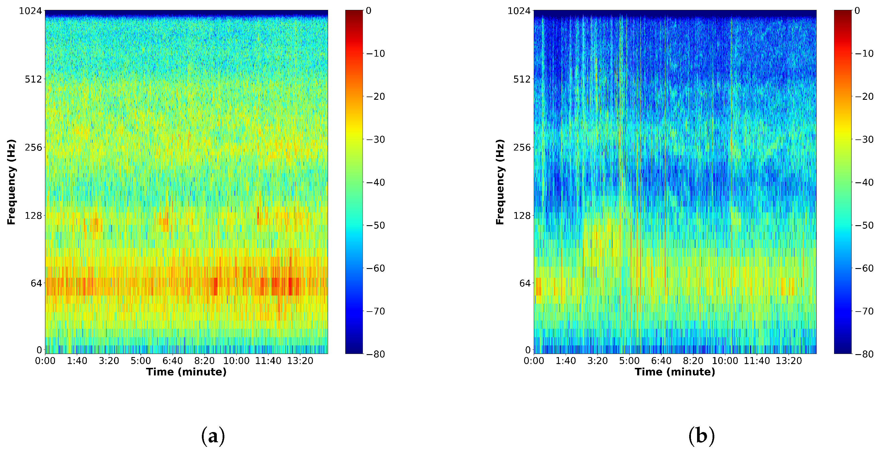
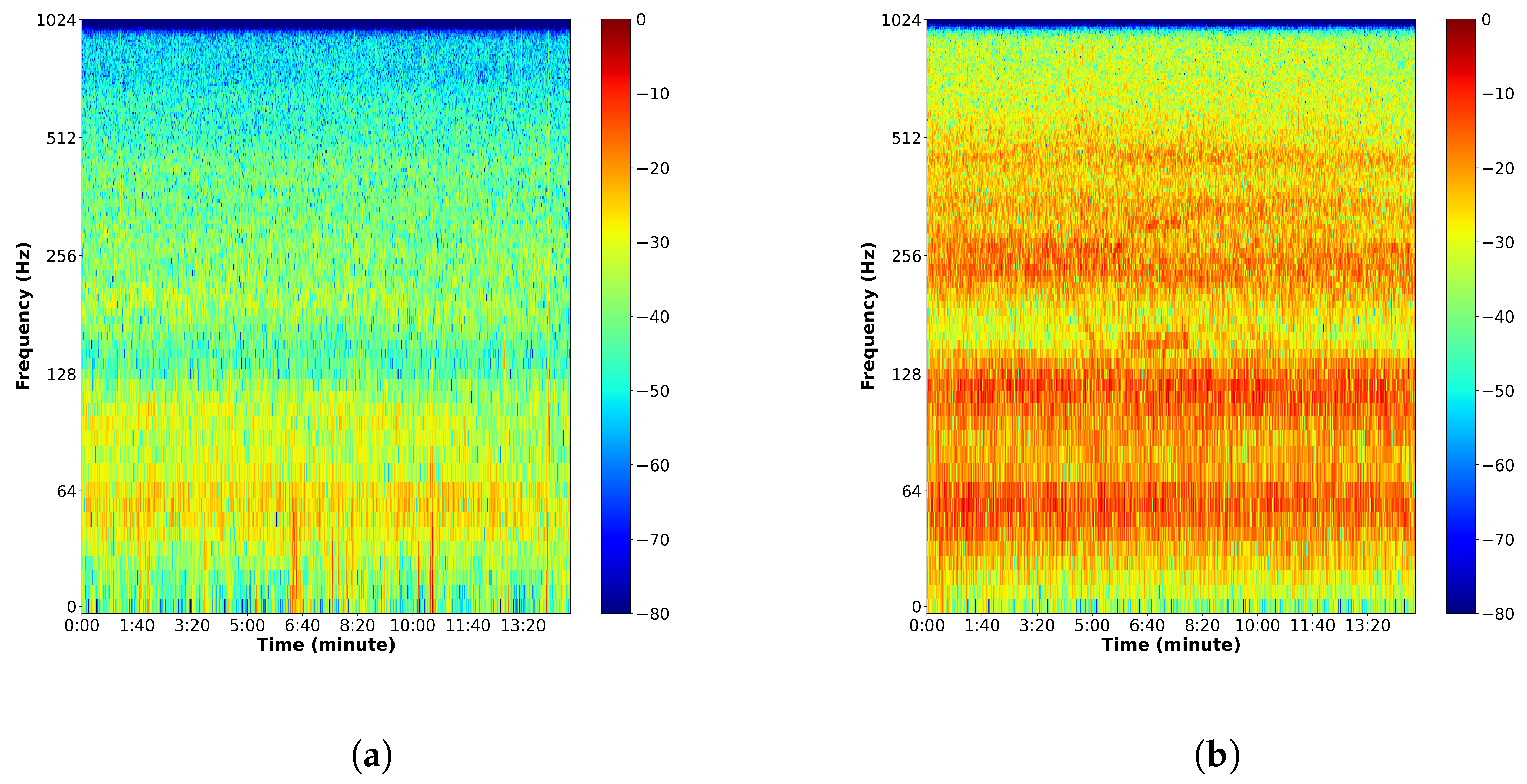
The moving RMS power is calculated based on Equation (1),
y R M S ( i ) = 1 N k = i i + N x ( k ) 2 , i = 0 , 1 , 2 , , L N 1
where L is the signal length and N the windowed segment length. In the speech-processing community, such a windowed segment is referred to as a “frame”. We use the same notation here, not to be confused with the frames within the beehive. As such, the term signal frame will be used henceforth. In this experiment, we set the signal frame length to 1 s and used 50% overlapping shifts.
Having access to the acoustics of an empty hive allows us to identify certain environmental factors that would be present in both the empty and the occupied hives. As shown in Figure 3a, the empty hive has a fairly constant value with noise-related fluctuations around this value, whereas the occupied hive has an increase in audio power during the day, which stabilizes around the afternoon and later drops in the evening. A close comparison between the two curves, however, shows events that are common in both boxes, thus signaling environmental factors that could affect the monitoring system. For example, after close investigation, it was found that the abrupt peaks seen in both curves were a train rail squealing from a passenger train that ran behind the building (1 km distance) in which the apiary was located or car horns from nearby traffic. The slower peaks, in turn, were related to beekeepers’ voices being recorded by the microphone when they spoke near the hive. Another environmental factor that appeared throughout the recordings was the noises of raindrops hitting the hive boxes on rainy days. A segment of data showing this factor is shown in Figure 3b. Given these three prominent environment noises, this paper investigated the impact that they have on three other popular audio features and an automated monitoring system based on them.

2.2.2. Spectrogram

A spectrogram is a time–frequency representation of the audio signal, and it has been widely used for swarming and queen absence detection [31,34]. The spectrogram is commonly measured with a short-time Fourier transform (STFT), where the signal is divided into equal-length segments by a moving window, and then each segment is transformed using the fast Fourier transform (FFT). In this study, a Hann window with a length of 125 ms with a 50% overlap was used. Figure 4 shows the spectrogram of a 24 h recording of the beehive previously shown in Figure 2 and Figure 3a. In the top figure, the × symbols depict the instances in which environmental noises were detected. From the bottom spectrogram plot, their influence on the spectrogram can be seen as sudden bursts of energy below 64 Hz, thus coinciding with important hive sounds that were present throughout the day.

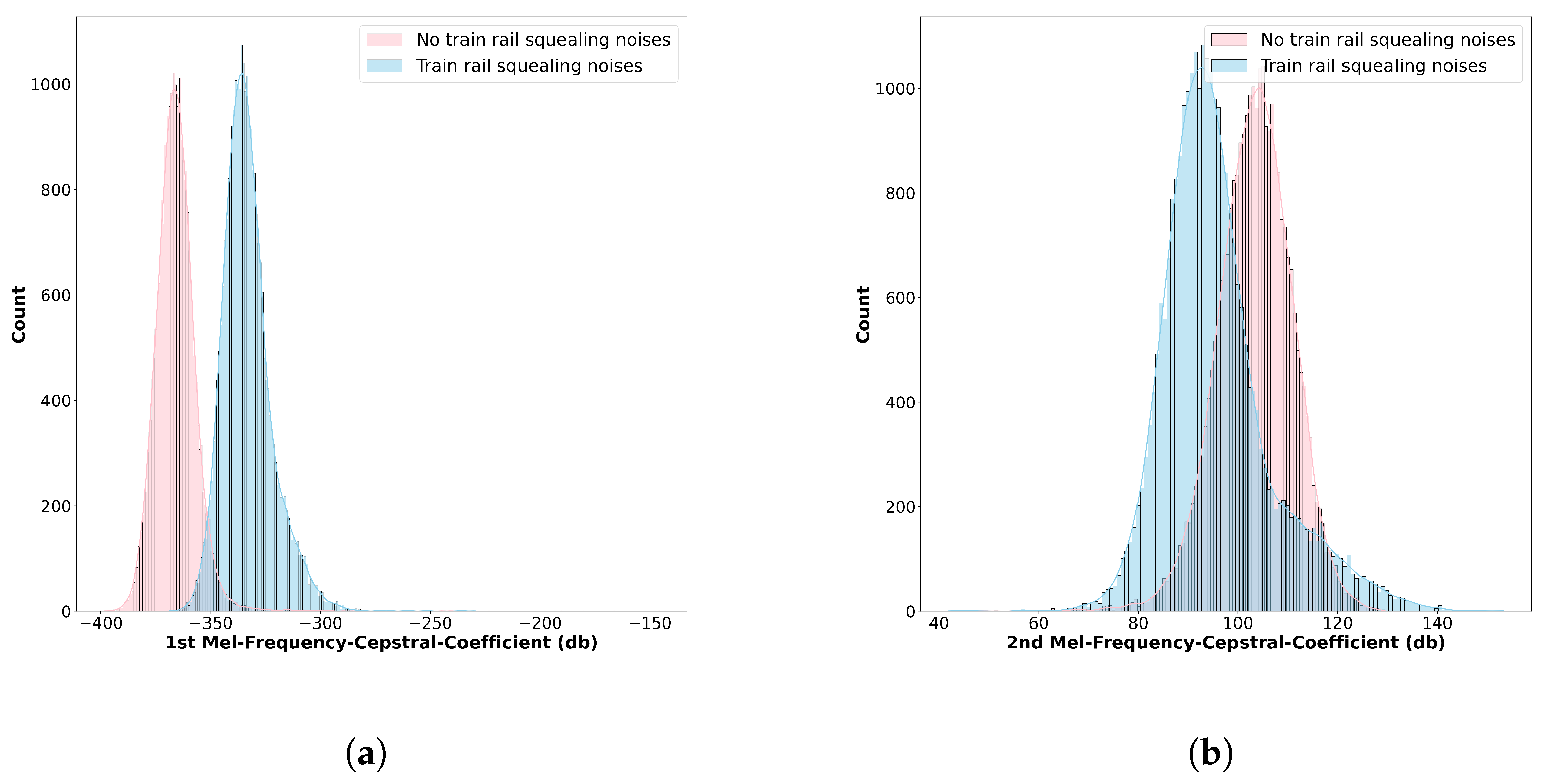
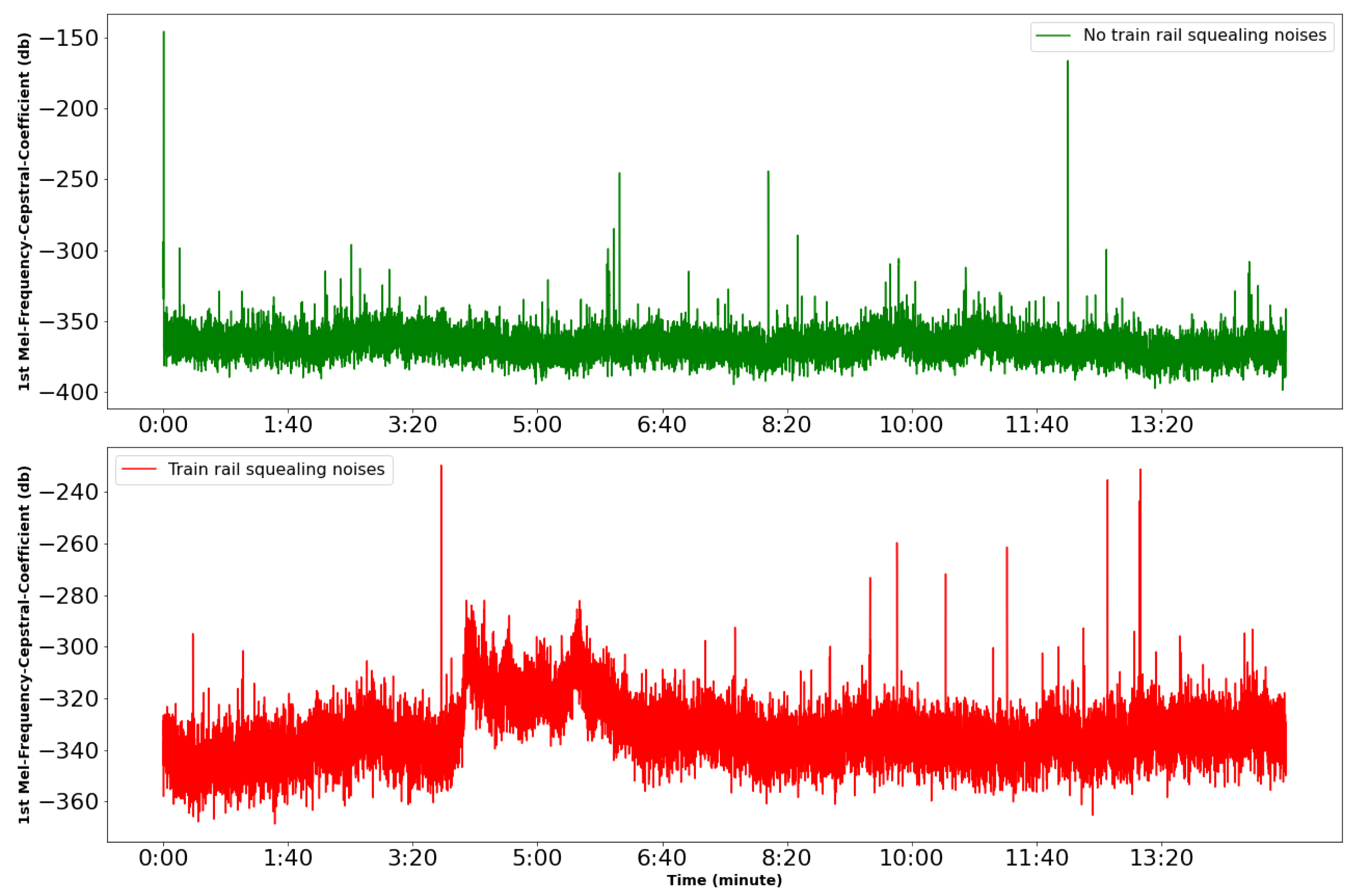
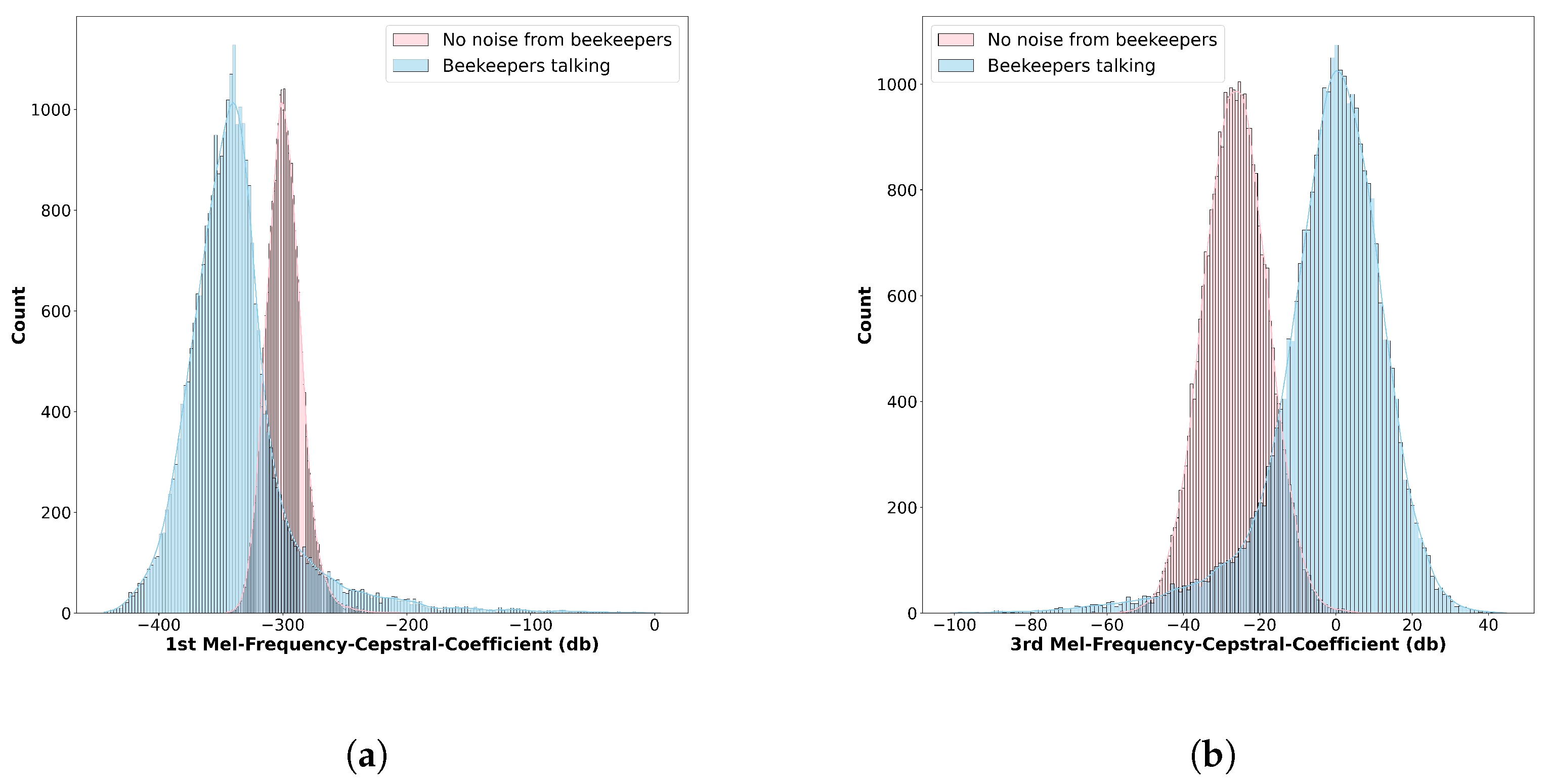
2.2.3. Mel-Frequency Cepstral Coefficients

MFCCs have been widely used in many speech applications, as they model the human cochlear processing steps by including a mel-scale frequency mapping prior to cepstrum processing [55]. For precision beekeeping, these features have also been shown to be popular, appearing in roughly 30% of the papers reviewed in [24]. For example, the first three MFCC coefficients have been widely used for bee, queen presence, and swarming detection. To calculate MFCCs, the following five steps were taken:
  • Apply a pre-emphasis filter to enhance high frequencies.
  • Compute the STFT of the pre-emphasized signal and its power spectrum.
  • Apply the mel filterbank, composed of triangular filters simulating cochlear processing.
  • Apply the logarithm operation.
  • Compute the discrete cosine transform (DCT) to extract the mel frequency cepstral coefficients.
In this experiment, a Hann window with a length of 125 ms with a 50% overlap was used in step 2. A total of 12 coefficients were extracted in step 5, plus the zeroth coefficient, which was used as a measure of signal power. Figure 5 shows the 12 MFCCs, plus the zeroth coefficient, as computed over the 24 h duration of the previous audio signal. In Section 3, more details will be provided on the effects of ambient noise on the MFCCs.

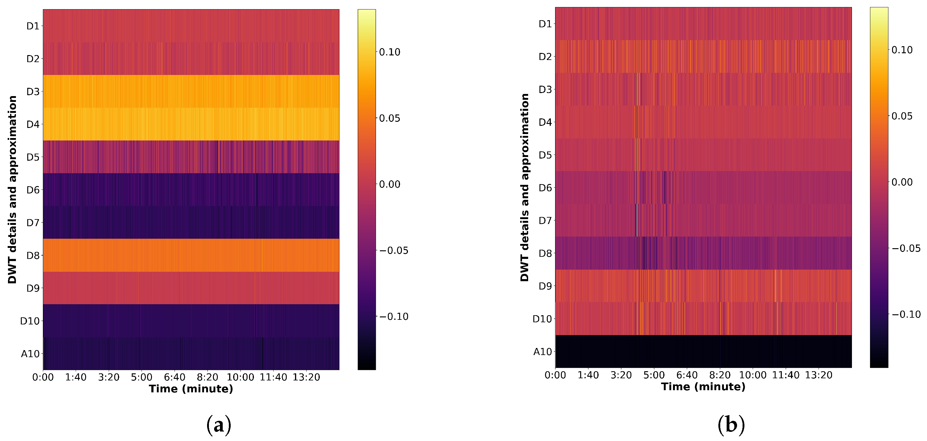
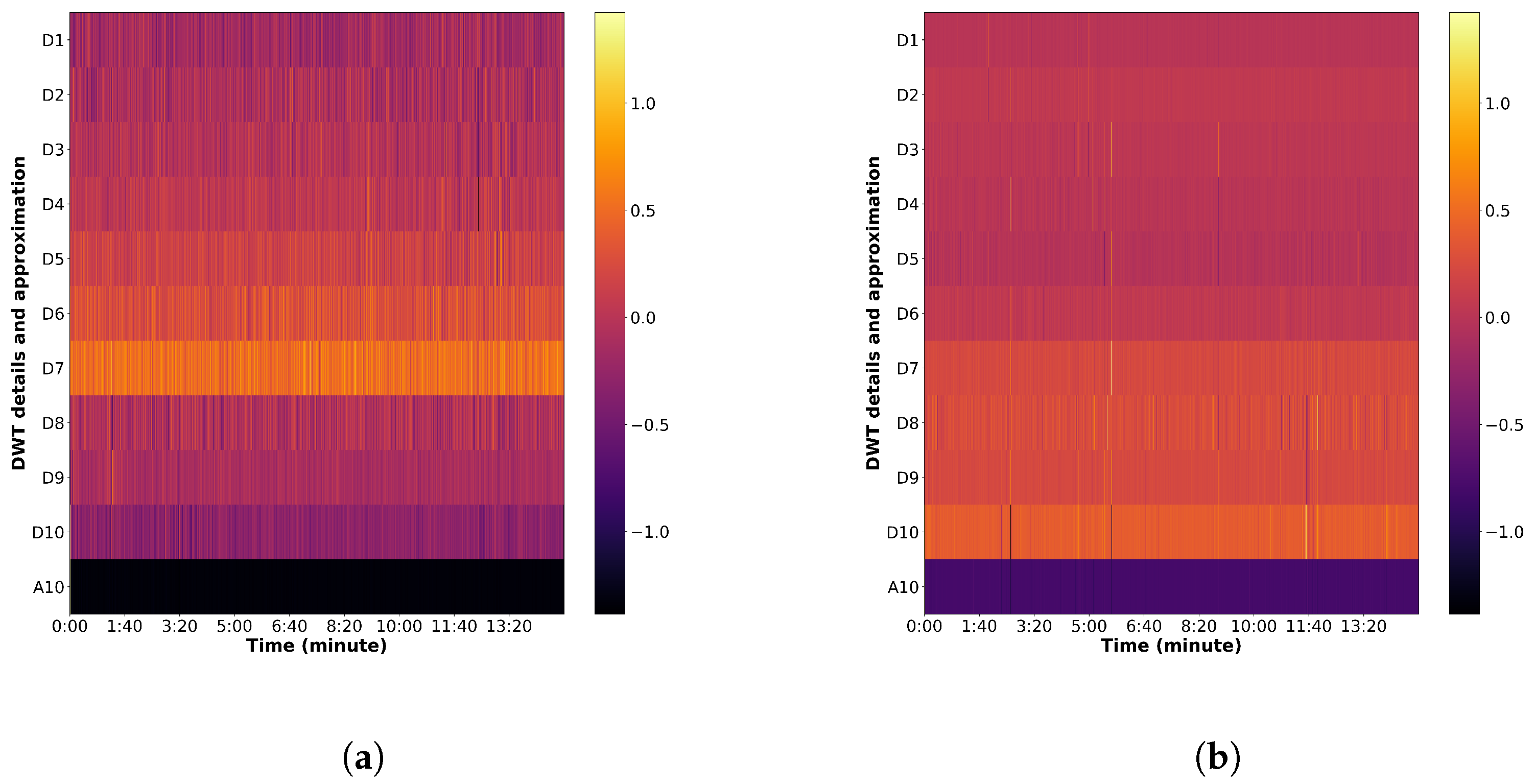
2.2.4. Discrete Wavelet Transform

Like the spectrogram, the DWT is a time–frequency representation that is widely used in time series analysis and has shown promising results for beehive acoustics monitoring applications [29,31]. DWTs rely on so-called wavelets to represent signals as a superposition of short finite-length waves that can be scaled and shifted to capture changes in the time–frequency space. The DWT is the discrete form of continuous wavelet transform (CWT) described by Equation (2):
C ( a , b ) = x ( t ) ψ a , b * ( t ) d t ,
where x ( t ) is the audio signal, ψ * is the complex conjugate of the mother wavelet ψ and a , b are the translation and scale, respectively. The mother wavelet is given by
ψ a , b ( t ) = 1 b ψ ( t a b ) .
In the DWT, the translation and scale values have the following conditions:
b = 2 s a = 2 s l ,
where l and s are discrete values.
Combining these conditions with the assumption of discretization of the signal results in the DWT shown in Equation (5), we obtain the following:
W ( l , s ) = 2 s 2 n x ( n ) ψ ( 2 s n 1 ) ; n = 0 , 1 , , L .
In this study, the audio is decomposed into an “approximation” and a “detail” component using a filtering implementation of the DWT [61]. In this case, a low-pass (G) and a high-pass (H) filter are used to separate the approximate ( A ( k ) ) and detail ( D ( k ) ) components of the signal, respectively:
A ( k ) = n x ( n ) h ( 2 k n ) , a n d
D ( k ) = n x ( n ) g ( 2 k n ) .
Here, we used the second order Daubechies wavelet [62] (“db2”) and 10 levels of decomposition based on combinations reported in the literature.
With these common features extracted for all 11 hives over three months, we used the empty hive and rainfall information to detect environmental sounds of interest and explore the effects they have on these features.

2.2.5. Modulation Spectrogram

The modulation spectrogram is a frequency–frequency representation that helps us to study the temporal dynamics of spectral components. Features extracted from the modulation spectrum have been used widely in human speech analysis, as they provide increased robustness against environment noise; representative examples include speaker identification [63] and speech emotion recognition [64], to name a few. If we consider the spectrogram as X ( t , f ) , the modulation spectrogram can be calculated as follows:
X ( f , f m o d ) = F t | X ( t , f ) | ,
where F t is a second Fourier transform computed across the time axis of the first time–frequency representation. The modulation spectrum is explored here as a potential tool for beehive context awareness.

2.3. Beehive Strength Prediction Model

To quantify the impact of the three environmental factors on beehive monitoring systems, three hive strength prediction models are developed, one based on each of the three feature sets described in Section 2.2. The goal of this monitoring system is to predict the number of frames of bees at any given point in time, thus serving as an indicator of the hive strength. In our case, a maximum of three boxes were included per hive, with each box containing 10 frames. As such, the model predicts a value between 0 and 30, where zero indicates an empty hive and 30 indicates that all three boxes are full.
Following recent insights from [24], a state-of-the-art convolutional deep neural network classifier was used. The three different two-dimensional time–frequency representations served as input to the classifier. Table 1 shows the network specifications. Each convolution layer has L2 regularization with a weight decay of 0.001 . All layers use a Rectified Linear Unit (ReLU) as an activation function, except the output layer, which uses a linear function. The best learning rate was found to be 0.001 , and the batch size was set to 128. Lastly, mean absolute error (MAE) was used as the loss function to train the network.

2.4. Experiment Setup and Figures-of-Merit

Audio data were recorded in 15-minute segments. These are divided into multiple 1-second signal frames, which were then used for feature extraction that served as input to the classifier. Following suggestions from [30,31], two different experimental setups are considered: “random-split” and “hive-independent”. In the former, the entire dataset from the 10 hives is randomly divided into three parts: 25% is for testing, 20% for validation and the rest is reserved for training. With the latter, a leave-some-hives-out setup was used. In particular, data from seven hives was used to train the models (of which 30% of the training data were set aside for validation), while the remaining three unseen hives were used for testing. This was repeated until all hives appeared in the test set.
For model evaluation, two figures-of-merit were used: mean absolute error (MAE) and the root mean square error (RMSE) obtained from the estimates and computed as follows, respectively, for a sample size of M:
MAE = n = 1 M | y i y ^ i | M ,
RMSE = n = 1 M ( y i y ^ i ) 2 M ,
where y is the observed value and y ^ the prediction.

3. Results and Discussion

3.1. Urban Sound Effects

As urban apiaries burgeon, common ambient sounds, such as car horns and train rail squealing, will become nuances for audio-based hive monitoring applications. As such, it is crucial to understand the impact that these sounds can have on the extracted audio features. For our study, sounds of a nearby train passing by was a common noise that contaminated the audio recordings. Figure 6, for example, shows the spectrogram measured from a 15-minute audio recording when the train was not passing by (subplot a), as well as when the train passed by (subplot b). As can be seen, the train rail squealing caused a significant disturbance in the audio around 64 Hz and higher frequencies such as 250 Hz, which is crucial for beehive dynamics.
Next, we explore the effects that such urban sounds may have on MFCCs. Figure 7 shows the histograms of the distribution of the first two coefficients (subplots and and b, respectively) across time instances in which the train sound was present versus absent. As can be seen, the train rail squealing sound has a substantial effect on the distribution of the MFCCs; in the case of the first coefficient, it increases the value by around 50 db. Such effects may result in erroneous decisions by automated systems that rely on the first three mel-frequency cepstral coefficients, such as the systems described in [3,30,31]. Figure 8 depicts the temporal changes seen in the first MFCC when the train passes by (see subplot b around the 5 min time). For systems that rely on average MFCCs over time, such increases will likely result in errors.
Lastly, Figure 9a,b depict the DWT detail (D1-D10) and approximation (A10) components extracted from the clean and noisy segments, respectively. As can be seen, the detailed coefficients are particularly affected by this urban noise source, and would likely result in errors for systems that rely on DWTs, such as the ones described in [29,31].

3.2. Speech Artifacts

Speech of people talking near the beehives is another common noise source when it comes to audio-based monitoring systems. Male speech, for example, is known to have fundamental frequencies ranging from 80 to 150 Hz, whereas female speech ranges from 160 to 250 Hz. These are typical ranges at which beehive acoustics are monitored, and thus the system performance could be severely compromised. The spectrograms in Figure 10b, for example, show scenarios in which speech is not present (plot a) near a particular hive and when beekeepers are talking near the same hive (plot b). Next, the histogram of the distribution of the first and third MFCCs shown in Figure 11 shows the impact due to speech artifacts. Similar changes in the DWT detail and approximation components can be seen in Figure 12.

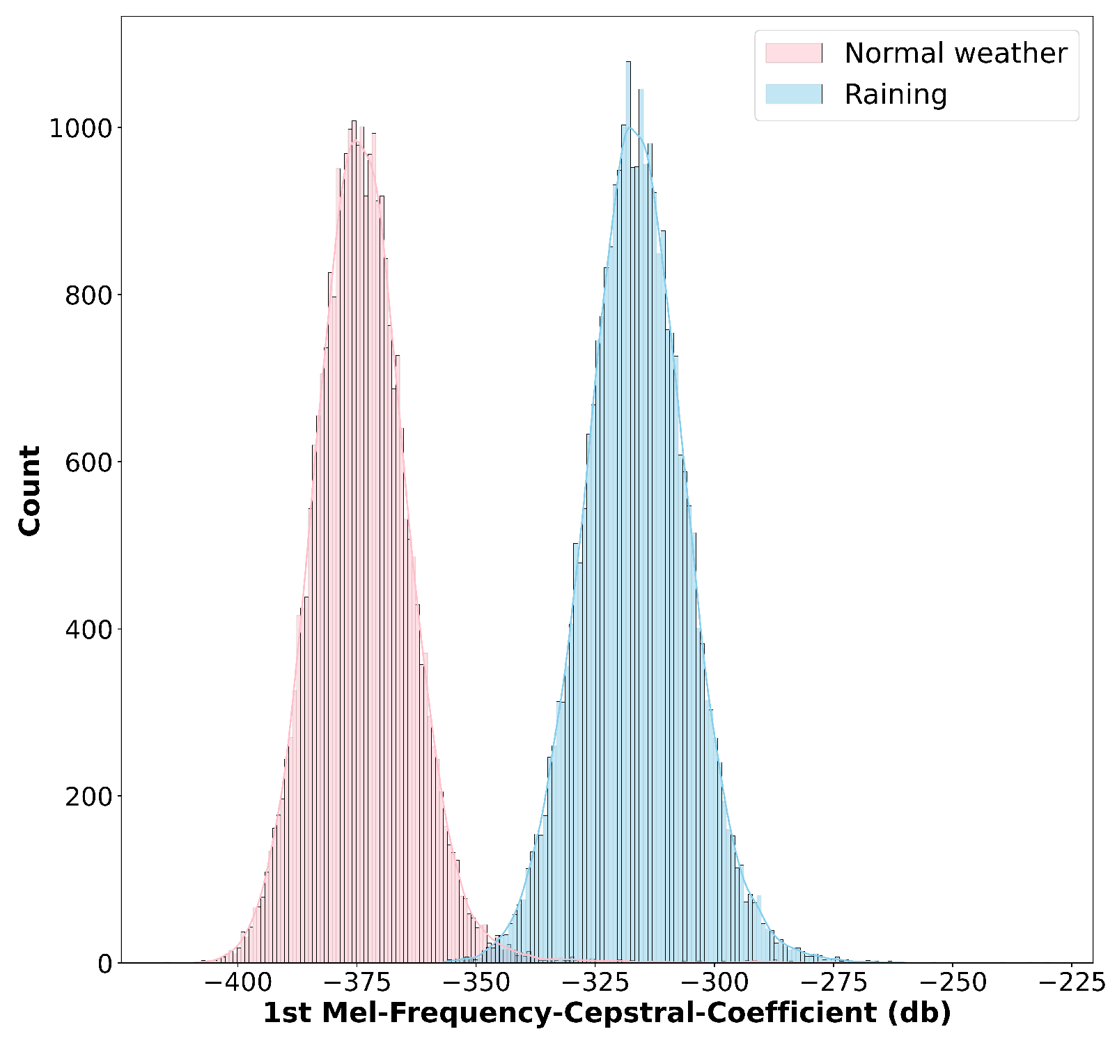
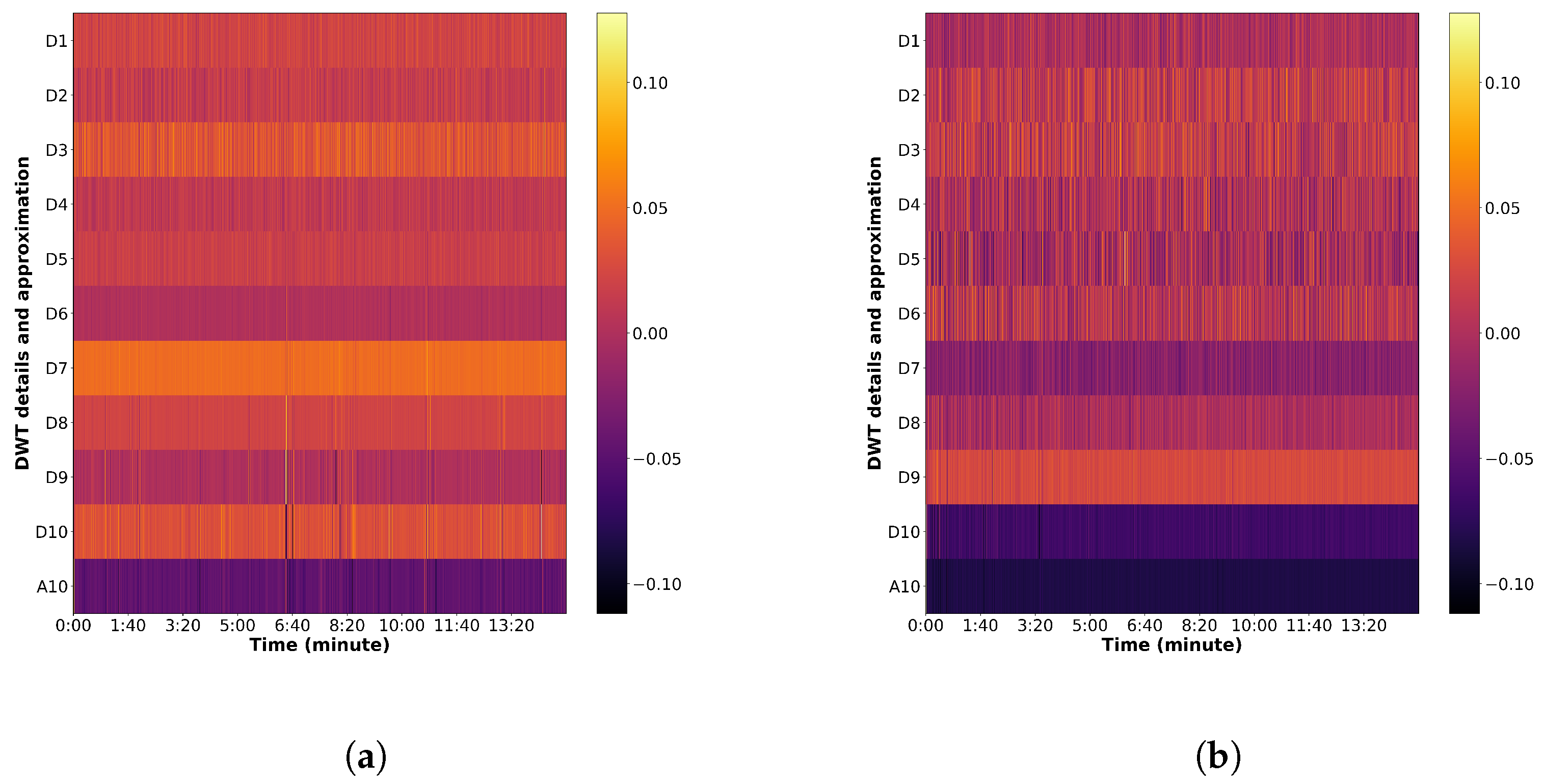
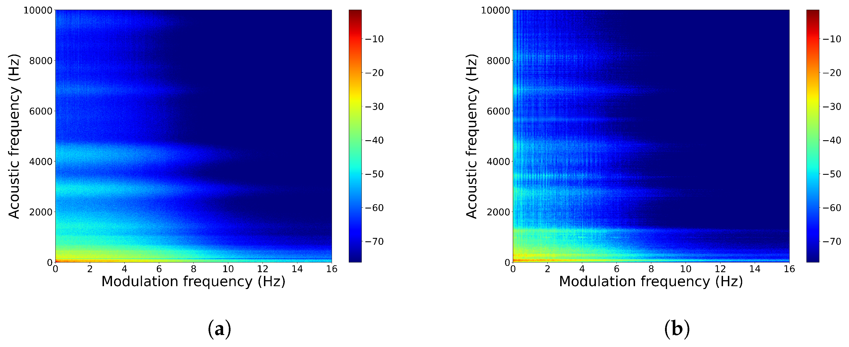
3.3. Acoustic Effects of Heavy Rain

Lastly, the sound of heavy rainfall hitting the hive boxes can also cause sufficient changes in the recorded audio to make monitoring systems fail. In our experiment, we relied on weather information to pinpoint periods of the day during which precipitation amounts greater than 9 mm were present. Figure 13 shows a comparison between the spectrograms of a hive during a typical night (plot a) and the same hive under heavy rainfall (plot b). As can be seen, rainfall sounds can severely affect multiple frequency ranges of the hive, increasing the recorded sound in some bands by as much as 10 dB, and thus is likely to deteriorate monitoring performance. The histogram of the distribution of the first MFCC shown in Figure 14 shows the impact that rainfall can have on this parameter. Lastly, Figure 15 shows the changes in the DWT components with and without rain artifacts. Unlike the urban and speech effects, which were transient and lasted a few seconds, rain sound can be much longer, potentially contaminating several hours of data, thus severely affecting the automated monitoring system.

3.4. Prediction Model Performance

Table 2 presents the prediction model performance when only clean test samples are available, as well as when the noisy samples are included. As can be seen, in the “random split” scenario, the system based on MFCCs outperformed the two other systems and achieved an MAE of 0.86 for the clean samples. When environmenta; factors were included, the DWT-based system was the most affected. Overall, MFCC-based systems achieved lower MAE under urban sound and heavy rain conditions, while the spectrogram-based system achieved lower MAE when speech was present. For the “hive-independent” setting, the three feature sets achieved similar results under clean conditions. The errors, however, are substantially larger than those achieved in the random-split case, suggesting great variability between hives. As mentioned previously, noise severely degraded performance. In this case, the spectrogram features achieved lower MAE for urban sounds and speech, whereas MFCCs performed better for heavy rain. In this setting, speech artifacts caused the most harm to monitoring systems. Taken together, these results highlight the potential of acoustics used in a machine learning framework and also the importance of context awareness for beehive monitoring to ensure that such environmental factors are taken into account during remote monitoring.

4. Recommendations

As shown above, environmental factors were shown to severely degrade beehive monitoring system performance based on acoustic signals. While the audio segments affected by heavy rain and train rail squealing sounds could potentially be detected based on weather stations’ information and/or train schedules, for example, detection of human speech was more challenging. Given the detrimental effect that human speech showed on hive-independent tests and colony behavior, an in-hive speech-detection system would be required. Here, we recommend the use of the modulation spectrum to detect such artifacts. The plots in Figure 16a,b show the modulation spectrogram of the audio data under clean conditions, as well as with background speech, respectively. Here, the original sampling rate of 48,000 Hz was used and a window length of 250 ms and window shift 31.25 ms was used to compute the modulation spectrum. As can be seen, the speech signal changed the dynamics of the audio below 8Hz modulation frequency (y axis), the region in which speech is known to be in. In future work, automated speech detectors and multimodal hive strength models using numerous sensors will be explored.

5. Conclusions

In this study, we collected audio, internal temperature, and internal humidity from 10 beehives and 1 empty hive in an urban apiary in Montréal, Canada. We showed the impact that three prominent noise sources (urban sounds, background speech, and heavy rain) had on three widely used features (spectrogram, MFCCs, and DWT). These impacts include significant changes in important bands of frequency in spectrogram, changes in the MFCCs distribution, especially in the first two coefficients, and lastly, distortion in the details and approximation DWT coefficients. These features were then used to train three separate hive-strength classifiers. The results indicated the potential of audio used in a deep learning model for predicting beehive population and health state, as the system based on MFCCs achieved an MAE of 0.86 for the clean samples. Tests using clean audio segments and noisy segments showed the sensitivity of the systems to environmental noise. We finalized the paper with recommendations on potential future works that could rely on new modulation spectral features for background beekeeper speech detection.

Author Contributions

Conceptualization, T.H.F. and P.G.; data collection, E.H.; methodology, T.H.F., P.G. and M.A.; writing—original draft preparation, M.A.; writing—review and editing, P.G., T.H.F. and E.H.; visualization, M.A.; supervision, T.H.F. and P.G.; funding acquisition, T.H.F. and P.G. All authors have read and agreed to the published version of the manuscript.

Funding

This work was made available through funding from NSERC Canada via its Alliance Grants program (ALLRP 548872-19) in partnership with Nectar Technologies Inc. and the Deschambault Animal Science Research Centre (CRSAD).

Institutional Review Board Statement

Not applicable.

Informed Consent Statement

Not applicable.

Data Availability Statement

Due to the sensitive nature of the data, information created during and/or analysed during the current study is available from the corresponding author on reasonable request to bona fide researchers.

Conflicts of Interest

The authors declare no conflict of interest.

References

  1. FAO; Apimondia; CAAS; IZSLT. Good Beekeeping Practices for Sustainable Apiculture; FAO: Rome, Italy, 2021.
  2. Hadjur, H.; Ammar, D.; Lefèvre, L. Toward an intelligent and efficient beehive: A survey of precision beekeeping systems and services. Comput. Electron. Agric. 2022, 192, 106604. [Google Scholar] [CrossRef]
  3. Ruvinga, S.; Hunter, G.J.; Duran, O.; Nebel, J.C. Use of LSTM Networks to Identify “Queenlessness” in Honeybee Hives from Audio Signals. In Proceedings of the 2021 17th International Conference on Intelligent Environments (IE), Dubai, United Arab Emirates, 21–24 June 2021; pp. 1–4. [Google Scholar]
  4. Dubois, S.; Choveton-Caillat, J.; Kane, W.; Gilbert, T.; Nfaoui, M.; El Boudali, M.; Rezzouki, M.; Ferré, G. Bee Detection For Fruit Cultivation. In Proceedings of the 2021 IEEE International Symposium on Circuits and Systems (ISCAS), Daegu, Republic of Korea, 22–28 May 2021; pp. 1–5. [Google Scholar]
  5. Peng, R.; Ardekani, I.; Sharifzadeh, H. An Acoustic Signal Processing System for Identification of Queen-less Beehives. In Proceedings of the 2020 Asia-Pacific Signal and Information Processing Association Annual Summit and Conference (APSIPA ASC), Auckland, New Zealand, 7–10 December 2020; pp. 57–63. [Google Scholar]
  6. Henry, E.; Adamchuk, V.; Stanhope, T.; Buddle, C.; Rindlaub, N. Precision apiculture: Development of a wireless sensor network for honeybee hives. Comput. Electron. Agric. 2019, 156, 138–144. [Google Scholar] [CrossRef] [Green Version]
  7. Cecchi, S.; Spinsante, S.; Terenzi, A.; Orcioni, S. A Smart Sensor-Based Measurement System for Advanced Bee Hive Monitoring. Sensors 2020, 20, 2726. [Google Scholar] [CrossRef] [PubMed]
  8. Braga, A.R.; Gomes, D.G.; Rogers, R.; Hassler, E.E.; Freitas, B.M.; Cazier, J.A. A method for mining combined data from in-hive sensors, weather and apiary inspections to forecast the health status of honey bee colonies. Comput. Electron. Agric. 2020, 169, 105161. [Google Scholar] [CrossRef]
  9. Meikle, W.G.; Rector, B.G.; Mercadier, G.; Holst, N. Within-day variation in continuous hive weight data as a measure of honey bee colony activity. Apidologie 2008, 39, 694–707. [Google Scholar] [CrossRef] [Green Version]
  10. Stalidzans, E.; Berzonis, A. Temperature changes above the upper hive body reveal the annual development periods of honey bee colonies. Comput. Electron. Agric. 2013, 90, 1–6. [Google Scholar] [CrossRef]
  11. Edwards-Murphy, F.; Magno, M.; Whelan, P.M.; O’Halloran, J.; Popovici, E.M. b+ WSN: Smart beehive with preliminary decision tree analysis for agriculture and honey bee health monitoring. Comput. Electron. Agric. 2016, 124, 211–219. [Google Scholar] [CrossRef]
  12. Hambleton, J. The quantitative and qualitative effect of weather upon colony weight changes. J. Econ. Entomol. 1925, 18, 447–448. [Google Scholar] [CrossRef]
  13. Cetin, U. The effects of temperature changes to bee losts. Uludag Bee J. 2004, 4, 171–174. [Google Scholar]
  14. Seeley, T.; Heinrich, B. Regulation of Temperature in the Nests of Social Insects; Wiley: Hoboken, NJ, USA, 1981. [Google Scholar]
  15. Seeley, T.D. Honeybee ecology. In Honeybee Ecology; Princeton University Press: Princeton, NJ, USA, 2014. [Google Scholar]
  16. Zacepins, A.; Kviesis, A.; Stalidzans, E.; Liepniece, M.; Meitalovs, J. Remote detection of the swarming of honey bee colonies by single-point temperature monitoring. Biosyst. Eng. 2016, 148, 76–80. [Google Scholar] [CrossRef]
  17. Abou-Shaara, H.; Owayss, A.; Ibrahim, Y.; Basuny, N. A review of impacts of temperature and relative humidity on various activities of honey bees. Insectes Sociaux 2017, 64, 455–463. [Google Scholar] [CrossRef]
  18. Human, H.; Nicolson, S.W.; Dietemann, V. Do honeybees, Apis mellifera scutellata, regulate humidity in their nest? Naturwissenschaften 2006, 93, 397–401. [Google Scholar] [CrossRef] [PubMed]
  19. Michelsen, A.; Kirchner, W.H.; Lindauer, M. Sound and vibrational signals in the dance language of the honeybee, Apis mellifera. Behav. Ecol. Sociobiol. 1986, 18, 207–212. [Google Scholar] [CrossRef]
  20. Hunt, J.; Richard, F.J. Intracolony vibroacoustic communication in social insects. Insectes Sociaux 2013, 60, 403–417. [Google Scholar] [CrossRef]
  21. Bromenshenk, J.J.; Henderson, C.B.; Seccomb, R.A.; Rice, S.D.; Etter, R.T. Honey bee acoustic recording and analysis system for monitoring hive health. US Patent 7,549,907, 23 June 2009. [Google Scholar]
  22. Zlatkova, A.; Kokolanski, Z.; Tashkovski, D. Honeybees swarming detection approach by sound signal processing. In Proceedings of the 2020 XXIX International Scientific Conference Electronics (ET), Sozopol, Bulgaria, 16–18 September 2020; pp. 1–3. [Google Scholar]
  23. Žgank, A. Acoustic monitoring and classification of bee swarm activity using MFCC feature extraction and HMM acoustic modeling. In Proceedings of the 2018 ELEKTRO, Moscow, Russia, 16–19 April 2018; pp. 1–4. [Google Scholar]
  24. Abdollahi, M.; Giovenazzo, P.; Falk, T.H. Automated Beehive Acoustics Monitoring: A Comprehensive Review of the Literature and Recommendations for Future Work. Appl. Sci. 2022, 12, 3920. [Google Scholar] [CrossRef]
  25. Heise, D.; Miller-Struttmann, N.; Galen, C.; Schul, J. Acoustic detection of bees in the field using CASA with focal templates. In Proceedings of the 2017 IEEE Sensors Applications Symposium (SAS), Glassboro, NJ, USA, 13–15 March 2017; pp. 1–5. [Google Scholar]
  26. Kim, J.; Oh, J.; Heo, T.Y. Acoustic Scene Classification and Visualization of Beehive Sounds Using Machine Learning Algorithms and Grad-CAM. Math. Probl. Eng. 2021, 2021, 5594498. [Google Scholar] [CrossRef]
  27. Nolasco, I.; Benetos, E. To bee or not to bee: Investigating machine learning approaches for beehive sound recognition. arXiv 2018, arXiv:1811.06016. [Google Scholar]
  28. Zhang, T.; Zmyslony, S.; Nozdrenkov, S.; Smith, M.; Hopkins, B. Semi-Supervised Audio Representation Learning for Modeling Beehive Strengths. arXiv 2021, arXiv:2105.10536. [Google Scholar]
  29. Terenzi, A.; Cecchi, S.; Orcioni, S.; Piazza, F. Features extraction applied to the analysis of the sounds emitted by honey bees in a beehive. In Proceedings of the 2019 11th International Symposium on Image and Signal Processing and Analysis (ISPA), Dubrovnik, Croatia, 23–25 September 2018; pp. 03–08. [Google Scholar]
  30. Nolasco, I.; Terenzi, A.; Cecchi, S.; Orcioni, S.; Bear, H.L.; Benetos, E. Audio-based identification of beehive states. In Proceedings of the ICASSP 2019-2019 IEEE International Conference on Acoustics, Speech and Signal Processing (ICASSP), Brighton, UK, 12–17 May 2019; pp. 8256–8260. [Google Scholar]
  31. Terenzi, A.; Ortolani, N.; Nolasco, I.; Benetos, E.; Cecchi, S. Comparison of Feature Extraction Methods for Sound-based Classification of Honey Bee Activity. IEEE/ACM Trans. Audio Speech Lang. Process. 2021, 30, 112–122. [Google Scholar] [CrossRef]
  32. Krzywoszyja, G.; Rybski, R.; Andrzejewski, G. Bee swarm detection based on comparison of estimated distributions samples of sound. IEEE Trans. Instrum. Meas. 2018, 68, 3776–3784. [Google Scholar] [CrossRef]
  33. Anand, N.; Raj, V.B.; Ullas, M.; Srivastava, A. Swarm Detection and Beehive Monitoring System using Auditory and Microclimatic Analysis. In Proceedings of the 2018 3rd International Conference on Circuits, Control, Communication and Computing (I4C), Bangalore, India, 3–5 October 2018; pp. 1–4. [Google Scholar]
  34. Zlatkova, A.; Gerazov, B.; Tashkovski, D.; Kokolanski, Z. Analysis of parameters in algorithms for signal processing for swarming of honeybees. In Proceedings of the 2020 28th Telecommunications Forum (TELFOR), Belgrade, Serbia, 24–25 November 2020; pp. 1–4. [Google Scholar]
  35. Qandour, A.; Ahmad, I.; Habibi, D.; Leppard, M. Remote Beehive Monitoring Using Acoustic Signals. Acoust. Aust. 2014, 42, 205. [Google Scholar]
  36. Sharif, M.Z.; Wario, F.; Di, N.; Xue, R.; Liu, F. Soundscape Indices: New Features for Classifying Beehive Audio Samples. Sociobiology 2020, 67, 566–571. [Google Scholar] [CrossRef]
  37. Zhao, Y.; Deng, G.; Zhang, L.; Di, N.; Jiang, X.; Li, Z. Based investigate of beehive sound to detect air pollutants by machine learning. Ecol. Inform. 2021, 61, 101246. [Google Scholar] [CrossRef]
  38. Pérez, N.; Jesús, F.; Pérez, C.; Niell, S.; Draper, A.; Obrusnik, N.; Zinemanas, P.; Spina, Y.M.; Letelier, L.C.; Monzón, P. Continuous monitoring of beehives’ sound for environmental pollution control. Ecol. Eng. 2016, 90, 326–330. [Google Scholar] [CrossRef]
  39. Hunter, G.; Howard, D.; Gauvreau, S.; Duran, O.; Busquets, R. Processing of multi-modal environmental signals recorded from a “smart” beehive. Proc. Inst. Acoust. 2019, 41, 339–348. [Google Scholar]
  40. Cecchi, S.; Terenzi, A.; Orcioni, S.; Riolo, P.; Ruschioni, S.; Isidoro, N. A preliminary study of sounds emitted by honey bees in a beehive. In Proceedings of the Audio Engineering Society Convention 144, Milan, Italy, 23–26 May 2018. [Google Scholar]
  41. Zacepins, A.; Kviesis, A.; Ahrendt, P.; Richter, U.; Tekin, S.; Durgun, M. Beekeeping in the future—Smart apiary management. In Proceedings of the 2016 17th International Carpathian Control Conference (ICCC), High Tatras, Slovakia, 29 May–1 June 2016; pp. 808–812. [Google Scholar]
  42. Imoize, A.L.; Odeyemi, S.D.; Adebisi, J.A. Development of a Low-Cost Wireless Bee-Hive Temperature and Sound Monitoring System. Indones. J. Electr. Eng. Inform. (IJEEI) 2020, 8, 476–485. [Google Scholar]
  43. Robles-Guerrero, A.; Saucedo-Anaya, T.; González-Ramírez, E.; De la Rosa-Vargas, J.I. Analysis of a multiclass classification problem by lasso logistic regression and singular value decomposition to identify sound patterns in queenless bee colonies. Comput. Electron. Agric. 2019, 159, 69–74. [Google Scholar] [CrossRef]
  44. Robles-Guerrero, A.; Saucedo-Anaya, T.; González-Ramérez, E.; Galván-Tejada, C.E. Frequency Analysis of Honey Bee Buzz for Automatic Recognition of Health Status: A Preliminary Study. Res. Comput. Sci. 2017, 142, 89–98. [Google Scholar] [CrossRef]
  45. Seeley, T.D.; Tautz, J. Worker piping in honey bee swarms and its role in preparing for liftoff. J. Comp. Physiol. A 2001, 187, 667–676. [Google Scholar] [CrossRef]
  46. Simpson, J.; Cherry, S.M. Queen confinement, queen piping and swarming in Apis mellifera colonies. Anim. Behav. 1969, 17, 271–278. [Google Scholar] [CrossRef]
  47. van der Zee, R.; Pisa, L.; Andonov, S.; Brodschneider, R.; Charriere, J.D.; Chlebo, R.; Coffey, M.F.; Crailsheim, K.; Dahle, B.; Gajda, A.; et al. Managed honey bee colony losses in Canada, China, Europe, Israel and Turkey, for the winters of 2008–9 and 2009–10. J. Apic. Res. 2012, 51, 100–114. [Google Scholar] [CrossRef] [Green Version]
  48. Jacques, A.; Laurent, M.; Consortium, E.; Ribière-Chabert, M.; Saussac, M.; Bougeard, S.; Budge, G.E.; Hendrikx, P.; Chauzat, M.P. A pan-European epidemiological study reveals honey bee colony survival depends on beekeeper education and disease control. PLoS ONE 2017, 12, e0172591. [Google Scholar] [CrossRef] [Green Version]
  49. Kulhanek, K.; Steinhauer, N.; Rennich, K.; Caron, D.M.; Sagili, R.R.; Pettis, J.S.; Ellis, J.D.; Wilson, M.E.; Wilkes, J.T.; Tarpy, D.R.; et al. A national survey of managed honey bee 2015–2016 annual colony losses in the USA. J. Apic. Res. 2017, 56, 328–340. [Google Scholar] [CrossRef] [Green Version]
  50. Brodschneider, R.; Gray, A.; Adjlane, N.; Ballis, A.; Brusbardis, V.; Charrière, J.D.; Chlebo, R.; Coffey, M.F.; Dahle, B.; de Graaf, D.C.; et al. Multi-country loss rates of honey bee colonies during winter 2016/2017 from the COLOSS survey. J. Apic. Res. 2018, 57, 452–457. [Google Scholar] [CrossRef] [Green Version]
  51. Gray, A.; Brodschneider, R.; Adjlane, N.; Ballis, A.; Brusbardis, V.; Charrière, J.D.; Chlebo, R.; Coffey, M.F.; Cornelissen, B.; Amaro da Costa, C.; et al. Loss rates of honey bee colonies during winter 2017/18 in 36 countries participating in the COLOSS survey, including effects of forage sources. J. Apic. Res. 2019, 58, 479–485. [Google Scholar] [CrossRef] [Green Version]
  52. Gray, A.; Adjlane, N.; Arab, A.; Ballis, A.; Brusbardis, V.; Charrière, J.D.; Chlebo, R.; Coffey, M.F.; Cornelissen, B.; Amaro da Costa, C.; et al. Honey bee colony winter loss rates for 35 countries participating in the COLOSS survey for winter 2018–2019, and the effects of a new queen on the risk of colony winter loss. J. Apic. Res. 2020, 59, 744–751. [Google Scholar] [CrossRef]
  53. Porrini, C.; Mutinelli, F.; Bortolotti, L.; Granato, A.; Laurenson, L.; Roberts, K.; Gallina, A.; Silvester, N.; Medrzycki, P.; Renzi, T.; et al. The status of honey bee health in Italy: Results from the nationwide bee monitoring network. PLoS ONE 2016, 11, e0155411. [Google Scholar] [CrossRef] [Green Version]
  54. Stanimirović, Z.; Glavinić, U.; Ristanić, M.; Aleksić, N.; Jovanović, N.; Vejnović, B.; Stevanović, J. Looking for the causes of and solutions to the issue of honey bee colony losses. Acta Vet. 2019, 69, 1–31. [Google Scholar] [CrossRef] [Green Version]
  55. Davis, S.; Mermelstein, P. Comparison of parametric representations for monosyllabic word recognition in continuously spoken sentences. IEEE Trans. Acoust. Speech Signal Process. 1980, 28, 357–366. [Google Scholar] [CrossRef] [Green Version]
  56. Barchiesi, D.; Giannoulis, D.; Stowell, D.; Plumbley, M.D. Acoustic scene classification: Classifying environments from the sounds they produce. IEEE Signal Process. Mag. 2015, 32, 16–34. [Google Scholar] [CrossRef]
  57. Gaballah, A.; Tiwari, A.; Narayanan, S.; Falk, T.H. Context-aware speech stress detection in hospital workers using Bi-LSTM classifiers. In Proceedings of the IEEE International Conference on Acoustics, Speech and Signal Processing, Toronto, ON, Canada, 6–12 June 2021; pp. 8348–8352. [Google Scholar]
  58. Stange, E. Optimizing urban beekeeping. In Achieving Sustainable urban Agriculture; Burleigh Dodds Science Publishing: Cambridge, UK, 2020; pp. 331–352. [Google Scholar]
  59. Nectar. Available online: https://www.nectar.buzz/ (accessed on 15 November 2022).
  60. Chabert, S.; Requier, F.; Chadoeuf, J.; Guilbaud, L.; Morison, N.; Vaissiere, B.E. Rapid measurement of the adult worker population size in honey bees. Ecol. Indic. 2021, 122, 107313. [Google Scholar] [CrossRef]
  61. Mallat, S.G. Multiresolution approximations and wavelet orthonormal bases of L2(R). Trans. Am. Math. Soc. 1989, 315, 69–87. [Google Scholar]
  62. Daubechies, I. Ten Lectures on Wavelets; SIAM: Philadelphia, PA, USA, 1992. [Google Scholar]
  63. Falk, T.H.; Chan, W.Y. Modulation spectral features for robust far-field speaker identification. IEEE Trans. Audio Speech Lang. Process. 2009, 18, 90–100. [Google Scholar] [CrossRef]
  64. Avila, A.R.; Monteiro, J.; O’Shaughneussy, D.; Falk, T.H. Speech emotion recognition on mobile devices based on modulation spectral feature pooling and deep neural networks. In Proceedings of the 2017 IEEE International Symposium on Signal Processing and Information Technology (ISSPIT), Bilbao, Spain, 18–20 December 2017; pp. 360–365. [Google Scholar]
Figure 1. Location of the (a) temperature and humidity sensor placed on top of the middle frame of the first brood chamber and (b) microphone placed next to it.
Applsci 13 00195 g001
Figure 2. Time series, from top to bottom, of audio intensity, audio RMS, internal/external temperature, and internal/external humidity readings in a hive with 3 boxes and 30 full frames of bees (date: 12 August 2021).
Applsci 13 00195 g002
Figure 3. RMS curves of a typical colony with three full boxes of bees (blue curve) and an empty box (orange) as measured on (a) 12 August 2021, and (b) 24 September 2021.
Applsci 13 00195 g003
Figure 4. RMS curve and corresponding spectrogram for a hive with with 3 full boxes of bees (12 August 2021).
Applsci 13 00195 g004
Figure 5. RMS curve and corresponding MFCCs for a hive with with 3 full boxes of bees (12 August 2021).
Applsci 13 00195 g005
Figure 6. Spectrograms of cases where urban noises (e.g., train rail squealing sounds) are (a) not present and (b) present.
Applsci 13 00195 g006
Figure 7. Comparison of the changes in distribution of the (a) first and (b) second mel frequency cepstral coefficient with and without the presence of train rail squealing sounds.
Applsci 13 00195 g007
Figure 8. First mel frequency cepstral coefficient time series when there are no trains nearby (top) versus when the train passes by (bottom) within the 4:00–6:40 time range.
Applsci 13 00195 g008
Figure 9. Comparison of the changes in distribution of the DWT detail and approximation components (a) without and (b) with the presence of train rail squealing sounds.
Applsci 13 00195 g009
Figure 10. Spectrogram comparisons when human speech is (a) not present and (b) present near the hives.
Applsci 13 00195 g010
Figure 11. Comparison of the changes in distribution of the (a) first and (b) third mel frequency cepstral coefficient with and without the presence of human speech.
Applsci 13 00195 g011
Figure 12. DWT detail and approximation component comparisons when human speech is (a) not present and (b) present near the hives.
Applsci 13 00195 g012
Figure 13. Spectrogram comparisons (a) without and (b) with heavy rainfalls.
Applsci 13 00195 g013
Figure 14. Comparison of the first MFCC histogram with and without rain.
Applsci 13 00195 g014
Figure 15. DWT component comparisons (a) without and (b) with heavy rainfalls.
Applsci 13 00195 g015
Figure 16. Modulation spectrogram of a segment, including (a) no noise and (b) speech artifacts.
Applsci 13 00195 g016
Table 1. Proposed convolutional neural network architecture.
LayerDescription
Convolution128 filters, kernel size = 3 × 3 , strides = 1 × 1
Batch normalizationmomentum = 0.99 , gamma = 1.0 , epsilon = 0.001
Max-poolingpool size = 3 × 3 , strides= 2 × 2
Convolution64 filters, kernel size = 3 × 3 , strides = 1 × 1
Batch normalizationmomentum = 0.99 , gamma = 1.0 , epsilon = 0.001
Convolution64 filters, kernel size = 3 × 3 , strides = 1 × 1
Batch normalizationmomentum = 0.99 , gamma = 1.0 , epsilon = 0.001
Max-poolingpool size = 3 × 3 , strides = 2 × 2
Dropout0.25 rate
Dense128 units
Batch normalizationmomentum = 0.99 , gamma = 1.0 , epsilon = 0.001
Dropout0.5 rate
Dense1 unit
Table 2. Performance comparison (MAE and RMSE) for beehive monitoring systems based on three feature sets under random-split and hive-independent testing scenarios.
Random-Split
FeaturesCleanUrban soundSpeech artifactsHeavy rain
MAERMSEMAERMSEMAERMSEMAERMSE
Spectrogram1.031.931.462.131.232.432.884.53
MFCCs0.862.341.172.721.863.931.002.52
DWT1.424.434.846.521.926.126.479.01
Hive-Independent
Spectrogram4.285.176.376.977.988.027.207.39
MFCCs4.915.736.937.868.779.236.957.75
DWT4.945.336.628.399.079.428.919.10
Disclaimer/Publisher’s Note: The statements, opinions and data contained in all publications are solely those of the individual author(s) and contributor(s) and not of MDPI and/or the editor(s). MDPI and/or the editor(s) disclaim responsibility for any injury to people or property resulting from any ideas, methods, instructions or products referred to in the content.

