Study on Mechanical Properties of Simply-Supported Composite Beams Considering Creep and Slip

Abstract

In the current industry, steel–concrete composite beams are used in large-span bridges and super-high-rise building structures due to their excellent overall performance. Concrete’s creep and slip effects in the combined structure can adversely affect the structure, thus affecting the safe use of bridges and buildings. It is necessary to study the mechanical properties of the combined structure considering creep and slip. In order to further study the mechanical properties of steel–concrete composite beams under creep–sliding coupling, in this study, based on the energy variational method principle, the energy equation of a composite beam considering creep and slip coupling is established. The second-order differential equation of the axial force of steel–concrete composite beams is derived by introducing basic assumptions. The calculation formulas for the axial force, deflection, and slip of simply-supported composite beams under different loads are obtained using different boundary conditions. Then, the creep effect of composite beams is simulated using the creep criterion in the ANSYS finite element software when the concrete material parameters change with time. The results show that a simply-supported composite beam considering both slip and creep will have a significant effect on the structure; the more strongly the studs constrain the concrete slab, the greater the adverse effect of concrete creep on the combined beam. The formula derived in this paper is consistent with the numerical simulation solution and is suitable for different creep and slip conditions. The research results can provide a theoretical basis for the calculation of the axial force, deflection, and slip of combined beams under uniform and concentrated loads in practical engineering considering slip and creep.

1. Introduction

Concrete and steel are the two primary materials of modern bridge engineering structures. Concrete has the characteristics of being a locally available raw material and having a lower cost and mature construction technology. It has been widely used in the construction of highway bridges for a long time. Steel structures have the advantages of uniformity, stability, light weight, industrialized production and assemblage, and recyclability. It is also a material utilized in bridges around the world. Steel and concrete composite beam structures can give full play to the performance of concrete and steel. Compared with concrete bridges, steel–concrete composite structure bridges are recyclable bridge structures. Ordinary steel–concrete composite beam bridges include composite beam bridges, composite truss bridges, composite steel frame bridges, composite arch bridges, and composite cable-stayed bridges [1].

The earliest research on the slip of composite beams originated in 1951. Newmark et al. [2] assumed that concrete slabs and steel beams were elastic materials, and the load–slip curves of shear connectors were linear. Based on this, the shear differential control equation at the interface of composite beams was established, and the analytical equation of the deflection curve ignoring the lifting effect was obtained. Then, in 1974, Adekola et al. [3] established the series solution of the deflection and in-plane stress equation of a concrete flange considering partial interaction in the constitutive interface equation and proved that the deflection was not affected by the interface interaction to a limited extent. In 1993, Girhammar et al. [4] presented an approximate expression for the deflection of composite beam structures under dynamic loading with partial interaction. In 1995, Oehlers et al. [5] discussed the influence of partial interaction on the shear connection strength of composite beams and the strain of steel beams. In 1999, Fabbrocino et al. [6] carried out a nonlinear numerical analysis of the structural behavior of a composite beam structure considering interface slip under a large bending moment by introducing the generalized relationship between the bending moment and curvature of the section.

Research on the creep of composite beams began in 1990. Italian scholars Tarantino et al. [7] studied the creep effect of composite beams with flexible shear connectors and proposed a viscoelastic analysis method for steel–concrete composite beams with flexible shear connectors. In 1993, Dezi et al. [8,9] also proposed the viscoelastic analysis method of steel–concrete continuous composite beams with flexible shear connectors and the variation in the redundant constraint response with time, caused by the creep shrinkage of concrete members. In 1995, Gilbert et al. [10] studied the time-dependent deformation of continuous beams under long-term loading due to the cracking of negative moment concrete slabs and the creep and shrinkage of concrete and proposed an analytical model. Finally, the measured results of full-scale experiments were in agreement with the calculations. In 1995, Dezi et al. [11] established a relationship equation reflecting the cooperative work between steel beams and concrete based on the viscoelastic analysis of prestressed composite beams and considering the shrinkage and creep of concrete. Then, in 1996, Dezi et al. [12] proposed a simplified time-varying analysis method for continuous composite beams with flexible shear connectors subjected to static loads, supporting the settlement, shrinkage, and prestress of concrete slabs. In 1997, Amadio et al. [13] proposed a simplified method for calculating the influence of shrinkage and creep in steel–concrete composite beams with rigid or flexible shear connections based on the age-adjusted effective modulus method. In 1997, Professor Nie et al. [14] from Tsinghua University studied and analyzed the steel–concrete composite beam, deduced the calculation formula of the long-term stress stiffness of concrete, and analyzed the influence of concrete shrinkage deformation on the steel beam section. In 2001, Dezi et al. [15] developed an analytical model for the shear-lag effect of composite beams with flexible shear connections, considering concrete’s long-term performance, which was established using the virtual work principle. In 2001, Zhou et al. [16] analyzed and deduced the calculation formula for internal force redistribution and double constraints in steel–concrete composite beams under the action of concrete shrinkage and creep. The concrete cracking in the negative moment zone of a steel–concrete composite continuous girder bridge was analyzed and discussed through an example. In 2003, Sheng et al. [17] established a formula for calculating the stress redistribution of prestressed steel–concrete composite beams under creep and selected a T-beam example for analysis. In 2003, Nie et al. [18] studied the degree of stiffness reduction in composite beams under specific constraints considering the slip effect.

In 2003, Jiang et al. [19] defined the constitutive interface relation by the Goodman elastic interlayer hypothesis and established the theoretical calculation equation of deflection and slip considering slip and shear effects according to the principle of minimum potential energy and the variational method. In 2004, Wang et al. [20] analyzed and measured steel–concrete composite beams considering the shrinkage and creep effect and the change in load structure in the construction process by using the effective modulus method adjusted by age and the finite element analysis method, and they proposed a new method to calculate the stress redistribution of steel–concrete composite beams under the action of shrinkage and creep. In 2004, Qiu et al. [21] established a particular element to consider the slip effect and a finite element analysis model of steel–concrete composite beams under shrinkage and creep effects using the age-adjusted effective modulus method. The long-term stress, deflection, and slip of steel–concrete composite beams were analyzed and calculated. The calculation results were reliable and consistent with the actual values. The creep effects, and the structural stress and strain, were numerically calculated and analyzed. In 2009, Fan et al. [22,23] studied the composite structure under shrinkage, creep, and cracking. In 2010 and 2016, Nguyen et al. [24,25] analyzed composite beams’ linear and nonlinear time correlation considering the creep and shrinkage effects of concrete flanges. They gave accurate spatial and temporal discrete deflection solutions considering the slip effect. In 2011, Miao et al. [26] considered the principle of minimum potential energy and the Goodman elastic interlayer hypothesis, and the analytic equation for the stress, deformation, and deflection of composite beam sections considering interlayer slip was derived. In 2019, Ji et al. [27] studied the deflection calculation method of steel–concrete composite beams. The research showed that when the stiffness of the shear connectors was less than 1200 MPa, the additional deflection caused by the interlayer slip effect was more extensive, and the influence on the total deflection was also more significant. The influence of the slip effect on the deflection of composite beams should be considered, and the smaller the shear stiffness, the greater the effect of interfacial slip on the deflection, so it is necessary to consider the combined effects of both concrete creep and interfacial slip on the combined beam.

There are many types of research on the finite element analysis of ordinary reinforced concrete beams, but there are few types of research on steel–concrete composite beams. The main reason is that many element forms exist in steel–concrete composite beams. Therefore, different elements should be selected to simulate various element components in steel–concrete structures, such as concrete, connectors, and steel beams. At the same time, the slip between concrete and steel beams and the concrete cracking in the negative moment zone of continuous composite beams should be considered. Therefore, most of the tests focus less on theoretical analysis for the study of steel–concrete composite beams. In 1997, Oven et al. [28] proposed a two-dimensional nonlinear finite element differential method based on the principle of virtual work to simulate simply-supported beams and continuous composite beams. In 1998, Salari et al. [29] proposed a new finite element method for composite beam elements with an unknown force. The Hermitian interpolation polynomial was used to cause the curvature to be linearly distributed, which reduced the solution’s accuracy to a certain extent. Therefore, the force-based model was more accurate than the displacement-based model. In 1999, Gattesco et al. [30] further proposed a four-node element in which each node has three degrees of freedom in the composite beam element. This assumption is different from other models in that the shear connector transfer is considered to be discontinuous and to fit the actual engineering state better. In 2000, Ayoub et al. [31] established an inelastic element based on the hybrid method. They analyzed the action of partially shear-connected composite beams under monotonic and cyclic loads. The model assumes that the spring is located at the element’s end, and the connection force is assumed to be linearly distributed within the element. In 2003, Qiu et al. [32] adopted the double-layer beam element analysis method, which regards the shear connector as a particular beam element. The two ends are rigidly connected with the steel beam and concrete to ensure that the two are bent together. Fang et al. [33] used the shear connector of the cantilever beam element to artificially increase the cross-sectional area of the connector to avoid excessive vertical deformation between the steel beam and the concrete slab. Wei [34] and others began to use spring elements to simulate shear connectors. Concrete and steel beams use three-dimensional solid elements to analyze composite beams’ deformation and elastic bearing capacity. In Miranda et al.’s work [35], the viscoelastic response of four steel concrete composite beams affected by changing environmental conditions was studied using a finite element model. The simulation results were basically consistent with the current formula, proving the applicability of the finite element model. In Sarfarazi et al. [36], the effects of crack separation and the bridge area on the tensile behavior of concrete were studied experimentally and numerically through the Brazilian tensile test. The visually observed failure process gained through numerical Brazilian tests was found to be very similar to that obtained through the experimental tests. Wang et al. [37] established a finite element model (FEM) of simply-supported composite slabs while considering the impacts of non-uniform shrinkage, cracking in the concrete, and the creep of the concrete; then, the reliability of the FEM was verified against the experimental data in the literature.

In summary, there are many experimental and theoretical studies on the slip problem of composite beams and the creep problem of concrete, proving that the study of slip and creep in the study of composite beams is very important. However, there are few studies on coupled creep and slip effects in composite beams. Most of the articles that have studied the creep of composite beams assume that the shear stiffness tends to infinity and ignore the effect of slip, but the results calculated in this way are subject to error. There is no formula for composite beams’ internal force and deformation considering the coupling calculation. Therefore, based on reasonable assumptions, this paper establishes and solves the second-order equilibrium differential equation of composite beams by using the variational energy method and minimum potential energy principle and obtains the calculation formulas for the axial force, deflection, and slip of composite beams under different load conditions. Then, we use large-scale finite element ANSYS software to perform slip and creep composite beam modeling analysis. The applicability of the formula derived in this paper is proven by comparing the numerical simulation solution with the analytical solution. This can provide a theoretical basis for the calculation of the axial forces, deflections, and slips of combined beams under uniform and concentrated loads considering slips and creep in practical engineering.

2. Coupling Analysis Considering the Slip and Creep Effect

The essence of the age-adjusted effective modulus method [13] is to use the integral mean value theorem to transform the integral Equation (1) of creep calculation into an algebraic equation that is convenient for calculation and to simplify the calculation while ensuring the calculation accuracy by introducing the aging coefficient.

$$\epsilon (t)=\frac{\sigma \left({\tau }_0\right)}{E}\left[1+\varphi \left(t,{\tau }_0\right)\right]+\frac{1}{E}{\displaystyle {\int }_{{\tau }_0}^t\frac{d\sigma (\tau )}{d\tau }}[1+\varphi (t,{\tau }_0)]d\tau$$

(1)

where $\epsilon (t)$ is the strain at time $t$;

$\sigma ({\tau }_0)$ is the instantaneous stress of concrete at time ${\tau }_0$;

$\varphi (t,{\tau }_0)$ is the calculation of the concrete creep coefficient at loading age ${\tau }_0$ considering age $t$;

$\sigma (t)$ is the instantaneous stress of concrete at time $t$.

Because integral calculation is very inconvenient, the integral mean value theorem is used to transform the more complex integral operation into an algebraic solution. The accuracy of the calculation results depends on the division of the integral interval. The two results will be infinitely close when the interval is divided into infinite hours.

It can be obtained from the integral mean value theorem that

$$\epsilon (t)=\frac{\sigma \left({\tau }_0\right)}{E}\left[1+\varphi \left(t,{\tau }_0\right)\right]+\frac{\sigma (t)-\sigma \left({\tau }_0\right)}{E}\left[1+\varphi \left(t,t_{\xi }\right)\right]$$

(2)

In the formula, ${\tau }_0\le t_{\xi }\le t$.

$$\varphi \left(t,t_{\xi }\right)=\frac{{\displaystyle {\int }_{{\tau }_0}^t\frac{d\sigma (\tau )}{d\tau }}\varphi (t,{\tau }_0)d\tau }{\sigma (t)-\sigma \left({\tau }_0\right)}$$

(3)

The introduction of the aging coefficient $\rho (t,{\tau }_0)$ shows

$$\varphi \left(t,t_{\xi }\right)=\rho \left(t,{\tau }_0\right)\varphi \left(t,{\tau }_0\right)$$

(4)

$$\rho \left(t,{\tau }_0\right)=\frac{{\displaystyle {\int }_{{\tau }_0}^t\frac{d\sigma (\tau )}{d\tau }}\varphi (t,{\tau }_0)d\tau }{[\sigma (t)-\sigma ({\tau }_0)]\varphi \left(t,{\tau }_0\right)}$$

(5)

$$\epsilon (t)=\frac{\sigma \left({\tau }_0\right)}{E}\left[1+\varphi \left(t,{\tau }_0\right)\right]+\frac{\sigma (t)-\sigma \left({\tau }_0\right)}{E}\left[1+\rho \left(t,{\tau }_0\right)\varphi \left(t,{\tau }_0\right)\right]$$

(6)

It can also be written as

$$\epsilon (t)=\frac{\sigma \left(t_0\right)}{E}\left[1+\varphi \left(t,{\tau }_0\right)\right]+\frac{\sigma (t)-\sigma (t_0)}{E_{\varphi }\left(t,{\tau }_0\right)}$$

(7)

$$E_{\varphi }(t,{\tau }_0)=\frac{E}{1+\rho (t,{\tau }_0)\varphi (t,{\tau }_0)}$$

(8)

Here, $E_{\varphi }(t,{\tau }_0)$ is the age-adjusted effective modulus.

Basic assumptions considering creep and slip in steel-concrete composite beams [38] are as follows:

• The concrete bridge deck and steel beam cross-sections are in accordance with the plane section assumption, and the shear connectors are equivalent to uniform continuous elastic media.
• The stress–strain relationship between the steel beam and concrete in the whole stress stage is linear, and the concrete is not cracked and spalls in the whole stress stage.
• We ignore the steel–concrete composite beam lift phenomenon. Without considering the transverse deformation, the curvatures of the concrete bridge deck and steel beam are equal.
• The influence of the shear-lag effect of the bridge deck on the deflection of the steel-concrete composite beam is ignored.

Establishment and Solution of the Control Differential Equation

The definition of the creep coefficient in China’s Code for Design of Highway Reinforced Concrete and Prestressed Concrete Bridges and Culverts’ (JTG 3362-2018) [39] is adopted.

$$\varphi \left(t,t_0\right)={\varphi }_0\cdot {\beta }_{\mathrm{c}}\left(t_0-t\right)$$

(9)

$${\varphi }_0={\varphi }_{\mathrm{RH}}\cdot \beta \left(f_{\mathrm{cm}}\right)\cdot \beta \left(t_0\right)$$

(10)

$${\varphi }_{\mathrm{RH}}=1+\frac{1-RH/R{H}_0}{0.46{\left(h/h_0\right)}^{1/3}}$$

(11)

$$\beta \left({\mathrm{f}}_{\mathrm{cm}}\right)=\frac{5.3}{{\left(f_{\mathrm{cm}}/f_{\mathrm{cm}0}\right)}^{0.5}}$$

(12)

$$\beta \left({\mathrm{t}}_0\right)=\frac{1}{0.1+{\left({\mathrm{t}}_0/{\mathrm{t}}_1\right)}^{0.2}}$$

(13)

$${\beta }_{\mathrm{c}}\left(t-t_0\right)={\left[\frac{\left(\mathrm{t}-{\mathrm{t}}_0\right)/{\mathrm{t}}_1}{{\beta }_{\mathrm{H}}+\left(\mathrm{t}-{\mathrm{t}}_0\right)/{\mathrm{t}}_1}\right]}^{0.3}$$

(14)

$${\beta }_{\mathrm{H}}=150\left[1+{\left(1.2\frac{RH}{R{H}_0}\right)}^{18}\right]\frac{h}{h_0}+250\le 1500$$

(15)

where $t_0$ is the concrete age at loading (d); $t$ is the calculation of the concrete age at the time of consideration (d);

$\varphi (t,t_0)$ is the loading age $t_0$ used to calculate the concrete creep coefficient considering age $t$;

${\varphi }_0$ is the nominal creep coefficient;

${\beta }_{\mathrm{c}}$ is the coefficient of creep development with time after loading;

$f_{\mathrm{cm}}$ is the average cylinder compressive strength (MPa) of strength grade C25~C50 concrete at 28 d age, $f_{\mathrm{cm}}=0.8f_{\mathrm{cu},\mathrm{k}}+8\mathrm{MPa}$;

$f_{\mathrm{cu},\mathrm{k}}$ is the age of 28 d, with a 95% guarantee rate of the concrete cube compressive strength standard value (MPa);

${\beta }_{\mathrm{RH}}$ is the coefficient related to annual average relative humidity;

$RH$ is the annual average relative humidity of the environment (%);

$h$ is the build’s theoretical thickness (mm), $h=2A/u$, $A$ is the build’s cross-sectional area, and the $u$ is build’s perimeter length in contact with the atmosphere.

$R{H}_0=100\%$;

$h_0=100\mathrm{mm}$;

$t_1=1d$;

$f_{\mathrm{cm}0}=10\mathrm{MPa}$.

Then, the age-adjusted effective modulus method is used to consider the influence of concrete creep, and the creep factor is introduced.

$$E_{\varphi }\left(t,t_0\right)=\frac{E_{\mathrm{c}}\left(t_0\right)}{1+{\psi }_t\varphi \left(t,t_0\right)}$$

(16)

In the formula, $E_{\varphi }(t,t_0)$ is the effective elastic modulus of concrete changing with time at loading age $t_0$; $E_{\mathrm{c}}\left(t_0\right)$ is the elastic modulus of concrete at loading age $t_0$; ${\psi }_t$ is the creep factor—namely, the simplified calculation of the aging factor $\rho (t,{\tau }_0)$ according to China’s Code for Design of Highway Steel Bridges under a permanent load to take 1.1; $\varphi (t,t_0)$ is the creep coefficient of concrete when the loading age is $t_0$, and the value of the creep coefficient refers to the provisions of the Code for Design of Highway Reinforced Concrete and Prestressed Concrete Bridges and Culverts.

Figure 1 and Figure 2 provide a general sense of the steel–concrete composite beam in the form of a transverse and longitudinal section diagram. Figure 3 shows an equivalent illustration of the stud connection between the interfaces of the combined beams, where ${\mathrm{k}}_{\mathrm{s}}$ is the stud stiffness.

From Figure 1 and Figure 2, the axial displacement of the bottom surface of the concrete slab can be expressed as

$${\dot{u}}_{\mathrm{c}}=u_{\mathrm{c}}-(h_{\mathrm{c}}/2)\theta$$

(17)

The axial displacement of the top surface of the steel beam can be expressed as

$${\dot{u}}_{\mathrm{s}}=u_{\mathrm{s}}-(h_{\mathrm{s}}/2)\theta$$

(18)

The slip between the interfaces of composite beams can be written as

$$s={\dot{u}}_{\mathrm{c}}-{\dot{u}}_{\mathrm{s}}=u_{\mathrm{c}}-u_{\mathrm{s}}+\theta d$$

(19)

In Equation (19), $d=\left(h_{\mathrm{c}}+h_{\mathrm{s}}\right)/2$.

The strain energy equation of the composite beam is established:

Strain energy of steel beam:

$${\mathsf{\Pi }}_{\mathrm{s}}=\frac{1}{2}{\displaystyle {\int }_0^l(E_{\mathrm{s}}{A}_{\mathrm{s}}}{\mu }_{\mathrm{s}}{{}^{\prime }}^2+E_{\mathrm{s}}{I}_{\mathrm{s}}{w^{″}}^2)dx$$

(20)

Strain energy of the concrete slab:

$${\mathsf{\Pi }}_{\mathrm{c}}=\frac{1}{2}{\displaystyle {\int }_0^l(E_{\varphi }{A}_{\mathrm{c}}}{\mu }_{\mathrm{c}}{{}^{\prime }}^2+E_{\varphi }{I}_{\mathrm{c}}{w^{″}}^2)dx$$

(21)

Elastic interlayer slip’s strain energy as in Figure 3:

$${\mathsf{\Pi }}_{\mathrm{sc}}=\frac{1}{2}{\displaystyle {\int }_0^l{k}_{\mathrm{s}}[({\mu }_{\mathrm{s}}}-{\mu }_{\mathrm{c}})+d\cdot w^{\prime }{]}^{2}dx$$

(22)

External load potential energy:

$${\mathsf{\Pi }}_{\mathrm{p}}={\displaystyle {\int }_0^{l}M(x)w^{″}}dx$$

(23)

where $E_{\mathrm{s}}$ is the elastic modulus of the steel beam; $h_{\mathrm{s}}$ is the height of the I-shaped steel beam; ${\mu }_{\mathrm{s}}$ is the axial horizontal displacement of the steel beam; $A_{\mathrm{s}}$ is the section area of the steel beam; $E_{\mathrm{c}}$ is the elastic modulus of concrete; $h_{\mathrm{c}}$ is the height of the concrete slab; ${\mu }_{\mathrm{c}}$ is the axial horizontal displacement of concrete; $A_{\mathrm{c}}$ is the cross-sectional area of concrete; $w$ is the deflection of the composite beam; $w^{\prime }$ is the corner $\theta$; $k_{\mathrm{s}}$ is the unit beam length slip stiffness, $k_{\mathrm{s}}=K/e$, $K$ is the single shear connector connection stiffness, and $e$ is the shear connector spacing.

Structural total potential energy equation:

$$\mathsf{\Pi }={\mathsf{\Pi }}_{\mathrm{s}}+{\mathsf{\Pi }}_{\mathrm{c}}+{\mathsf{\Pi }}_{\mathrm{sc}}+{\mathsf{\Pi }}_{\mathrm{p}}$$

(24)

Substitute Equations (20)–(23) into Equation (24) to obtain

$$\begin{array}{ll}\mathsf{\Pi }=& \frac{1}{2}{\displaystyle {\int }_0^l(E_{\mathrm{s}}{A}_{\mathrm{s}}}{\mu }_{\mathrm{s}}{{}^{\prime }}^2+E_{\mathrm{s}}{I}_{\mathrm{s}}{w^{″}}^2+E_{\mathrm{c}}{A}_{\mathrm{c}}{\mu }_{\mathrm{c}}{{}^{\prime }}^2+E_{\varphi }{I}_{\mathrm{c}}{w^{″}}^2\\ & +k_{\mathrm{s}}{[({\mu }_{\mathrm{s}}-{\mu }_{\mathrm{c}})+d\cdot w^{\prime }]}^2)dx+{\displaystyle {\int }_0^{l}M(x)w^{″}}dx\end{array}$$

(25)

According to the principle of minimum potential energy, let $\delta \mathsf{\Pi }=0$:

$$\begin{array}{ll}\delta \mathsf{\Pi }=& {\displaystyle {\int }_0^l(E_{\mathrm{s}}{A}_{\mathrm{s}}}{\mu }_{\mathrm{s}}{}^{\prime }\delta {\mu }_{\mathrm{s}}{}^{\prime }+E_{\mathrm{s}}{I}_{\mathrm{s}}{w}^{″}\delta w^{″}+E_{\varphi }{A}_{\mathrm{c}}{\mu }_{\mathrm{c}}{}^{\prime }\delta {\mu }_{\mathrm{c}}{}^{\prime }+E_{\varphi }{I}_{\mathrm{c}}{w}^{″}\delta w^{″}+\\ & k_{\mathrm{s}}[({\mu }_{\mathrm{s}}-{\mu }_{\mathrm{c}})+d\cdot w^{\prime }]\delta [({\mu }_{\mathrm{s}}-{\mu }_{\mathrm{c}})+d\cdot w^{\prime }]+M(x)\delta w^{″})dx=0\end{array}$$

(26)

The governing differential equations and boundary conditions can be obtained by integral by parts for Equation (26):

$$\{\begin{array}{c}EI{w}^{‴}+M^{\prime }(x)-k_{\mathrm{s}}d[({\mu }_{\mathrm{s}}-{\mu }_{\mathrm{c}})+d\cdot w^{\prime }]=0\\ E_{\mathrm{s}}{A}_{\mathrm{s}}{\mu }_{\mathrm{s}}{}^{″}-k_{\mathrm{s}}[({\mu }_{\mathrm{s}}-{\mu }_{\mathrm{c}})+d\cdot w^{\prime }]=0\\ E_{\varphi }{A}_{\mathrm{c}}{\mu }_{\mathrm{c}}{}^{″}+k_{\mathrm{s}}[({\mu }_{\mathrm{s}}-{\mu }_{\mathrm{c}})+d\cdot w^{\prime }]=0\\ [EI{w}^{″}+M(x)]\delta w^{\prime }|\begin{array}{c}l\\ 0\end{array}=0\\ E_{\mathrm{s}}{A}_{\mathrm{s}}{\mu }_{\mathrm{s}}{}^{\prime }\delta {\mu }_{\mathrm{s}}|\begin{array}{c}l\\ 0\end{array}=0\\ E_{\varphi }{A}_{\mathrm{c}}{\mu }_{\mathrm{c}}{}^{\prime }\delta {\mu }_{\mathrm{c}}|\begin{array}{c}l\\ 0\end{array}=0\end{array}$$

(27)

In Equation (27), $EI=E_{\mathrm{s}}{I}_{\mathrm{s}}+E_{\varphi }{I}_{\mathrm{c}}$.

The second and third derivatives in Equation (27) can be obtained:

$$E_{\mathrm{s}}{A}_{\mathrm{s}}{\mu }_{\mathrm{s}}{}^{‴}-k_{\mathrm{s}}[({\mu }_{\mathrm{s}}{}^{\prime }-{\mu }_{\mathrm{c}}{}^{\prime })+d\cdot w^{″}]=0$$

(28)

$$E_{\varphi }{A}_{\mathrm{c}}{\mu }_{\mathrm{c}}{}^{‴}+k_{\mathrm{s}}[({\mu }_{\mathrm{s}}{}^{\prime }-{\mu }_{\mathrm{c}}{}^{\prime })+d\cdot w^{″}]=0$$

(29)

It can be known from the axial force balance condition that

$$N=N_{\mathrm{s}}=-N_{\mathrm{c}}=E_{\mathrm{s}}{A}_{\mathrm{s}}{\mu }_{\mathrm{s}}{}^{\prime }=-E_{\varphi }{A}_{\mathrm{c}}{\mu }_{\mathrm{c}}{}^{\prime }$$

(30)

Substituting Equation (30) into Equation (28), we can obtain

$$N^{″}-k_{\mathrm{s}}(\frac{1}{EA})N-k_{\mathrm{s}}d{w}^{″}=0$$

(31)

In the formula, $\frac{1}{EA}=\frac{1}{E_{\mathrm{s}}{A}_{\mathrm{s}}}+\frac{1}{E_{\varphi }{A}_{\mathrm{c}}}$.

According to the relationship between the bending moment and curvature,

$$EI{w}^{″}-Nd=M$$

(32)

Substituting Equation (32) into Equation (31), we can obtain

$$N^{″}-k_{\mathrm{s}}(\frac{1}{EA}+\frac{d^2}{EI})N=k_{\mathrm{s}}\frac{d}{EI}M$$

(33)

This can be simplified to obtain

$$N^{″}-\frac{k_{\mathrm{s}}}{EA}(1+\frac{EA{d}^2}{EI})N=k_{\mathrm{s}}\frac{d}{EI}M$$

(34)

Simplifying Equation (34) by ${\alpha }^2=\frac{k_{\mathrm{s}}(1+\beta )}{EA}$, $\beta =\frac{EA{d}^2}{EI}$, $\gamma =\frac{\beta }{d(1+\beta )}$, the governing differential equation with axial force N as an unknown function can be obtained:

$$N^{″}-{\alpha }^{2}N={\alpha }^2\gamma M$$

(35)

2.1. Analytical Solution of Axial Force

Axial force equation under uniform load:

Figure 4 shows the uniformly distributed load diagram established with the left support as the origin and along the length of the beam in the X direction.

Figure 4 shows that the bending moment equation of the simply-supported beam is

$$M\left(x\right)=\frac{q}{2}x(l-x),0\le x\le l$$

(36)

By the boundary conditions $x=0$, $N=0$, when $x=l$, $N=0$, the axial force equation under a uniform load can be obtained by substituting Equation (36) into Equation (35) and integrating them twice:

$$N(x)=\gamma M(x)+\frac{q\gamma }{{\alpha }^2}\left\{\frac{\cosh (\alpha (L/2-x))}{\cosh (\alpha L/2)}-1\right\}$$

(37)

Axial force equation under concentrated load:

Figure 5 shows the concentrated load diagram established with the left support as the origin and along the length of the beam in the X direction.

Figure 5 shows that the bending moment equation of the simply-supported beam is

$$M\left(x\right)=\{\begin{array}{l}{M}_1=\frac{Px}{2},0\le x\le l/2\\ M_2=\frac{P\left(l-x\right)}{2},l/2\le x\le l\end{array}$$

(38)

By the boundary conditions $x=0$, $N=0$, when $x=l$, $N=0$, substituting Equations (39) and (40) into Equation (35) and integrating them twice, the equation of axial force $N$ under a uniform load can be obtained:

$$N_1(x)=\gamma M_1-\frac{1}{2}\frac{\gamma P\sinh (\alpha x)}{\alpha \cosh (\alpha L/2)}$$

(39)

$$N_2(x)=\gamma M_2-\frac{1}{2}\frac{\gamma P\sinh (\alpha (L-x))}{\alpha \cosh (\alpha L/2)}$$

(40)

2.2. Analytical Solution of Deflection

Deflection equation under uniform load:

In the case of a known structural form and load, the deflection equation of (41) can be obtained by twice the integral of the boundary conditions.

$$f(x)={\displaystyle \iint \frac{M(x)+N(x)d}{EI}}dxdx$$

(41)

The bending moment equation of the simply-supported beam can be seen in Figure 4.

$$M\left(x\right)=\frac{q}{2}x(l-x),0\le x\le l$$

(42)

By the boundary conditions $x=0$, $f=0$, when $x=l$, $f=0$, and using Equations (42), (41), and (35), the deflection f equation of the simply-supported beam under a uniform load can be obtained as follows:

$$\begin{array}{l}f=\frac{q}{24EI(1+\beta )}\left(x^4-2l{x}^3+l^{3}x\right)+\\ \frac{q\gamma d}{{\alpha }^{4}EI}\left(\frac{\cosh (\alpha (l/2-x))}{\cosh (\alpha l/2)}-1\right)+\frac{q\gamma d}{2{\alpha }^{2}EI}\left(lx-x^2\right)\end{array}$$

(43)

Deflection equation under concentrated load:

The bending moment equation of the simply-supported beam can be seen in Figure 5:

$$M\left(x\right)=\{\begin{array}{l}{M}_1=\frac{Px}{2},0\le x\le l/2\\ M_2=\frac{P\left(l-x\right)}{2},l/2\le x\le l\end{array}$$

(44)

By the boundary conditions $x=0$, $f=0$, when $x=l$, $f=0$, and using Equations (44), (41), and (35), the deflection f equation of the simply-supported beam under a uniform load can be obtained as follows:

$$f_1=\frac{P\left(-\frac{1}{12}{x}^3+\frac{1}{16}{l}^{2}x\right)}{EI(1+\beta )}+\frac{1}{2}\frac{\gamma dPx}{{\alpha }^{2}EI}-\frac{1}{2}\frac{\gamma dP\sinh (\alpha x)}{{\alpha }^3\cosh \left(\frac{1}{2}\alpha L\right)EI}$$

(45)

$$f_2=\frac{P\left(\frac{1}{12}{x}^3-\frac{1}{4}l{x}^2+\frac{3}{16}{l}^{2}x-\frac{1}{48}{l}^3\right)}{EI(1+\beta )}+\frac{1}{2}\frac{P\gamma d(l-x)}{{\alpha }^{2}EI}-\frac{1}{2}\frac{P\gamma d\sinh (\alpha (l-x))}{{\alpha }^{3}EI\cosh \left(\frac{1}{2}\alpha l\right)}$$

(46)

2.3. Analytical Solution of Slip

According to the second item of (27),

$$E_{\mathrm{s}}{A}_{\mathrm{s}}{\mu }_{\mathrm{s}}{}^{″}-k_{\mathrm{s}}[({\mu }_{\mathrm{s}}-{\mu }_{\mathrm{c}})+d\cdot w^{\prime }]=0$$

(47)

From Equations (19) and (30), $S=u_{\mathrm{s}}-u_{\mathrm{c}}+d\cdot w^{\prime }$ and $N^{\prime }=E_{\mathrm{s}}{A}_{\mathrm{s}}{\mu }_{\mathrm{s}}{}^{″}$ are substituted into Equation (47):

$$S=\frac{N^{\prime }}{k_{\mathrm{s}}}$$

(48)

Slip equation under uniform load:

Substituting Equation (37) into Equation (48), the equation solution of slip under a uniform load can be obtained:

$$S(x)=\frac{\gamma q}{k_{\mathrm{s}}\alpha }\left[\frac{\sinh (\alpha (L/2-x))}{\cosh (\alpha L/2)}-\alpha (L/2-x)\right]$$

(49)

Slip equation under concentrated load:

Substituting Equations (39) and (40) into Equation (48), the equation solution of slip under a concentrated load can be obtained:

$$S_1(x)=\frac{\gamma P}{k_{\mathrm{s}}}\left[\frac{\sinh (\alpha L/2)}{\sinh (\alpha L)}\cosh (\alpha x)-\frac{1}{2}\right]$$

(50)

$$S_2(x)=\frac{\gamma P}{k_{\mathrm{s}}}\left[\frac{1}{2}-\frac{\sinh (\alpha L/2)}{\sinh (\alpha L)}\cosh (\alpha (L-x))\right]$$

(51)

3. ANSYS Finite Element Software Modeling Analysis

3.1. Selection of Modeling Unit

In the ANSYS finite element software, the studs considering slip between composite beam interfaces are simulated by the Combin39 spring element. The concrete slab and the steel beam flange are simulated by solid elements Solid65 and Solid45, respectively, and the steel beam web is simulated by plate element Plane42 (Figure 6) [40].

3.2. Implicit Creep Method

The implicit creep analysis method supports the following elements: Plane42, Solide45, Beam188, and Beam189.

In the implicit creep method, ANSYS uses the TBOPT command to select its own equations in the software, such as the following.

(1)

TBOPT = 1 Initial creep equation

$${\epsilon }_{\mathrm{cr}}=C_1{\sigma }^{C_2}{\epsilon }_{\mathrm{cr}}{}^{C_3}{e}^{-C_4/T}$$

(52)

(2)

TBOPT = 6 Initial creep equation

$${\epsilon }_{\mathrm{cr}}=C_1{\sigma }^{C_2}{\epsilon }_{\mathrm{cr}}{}^{C_3+1}{e}^{-C_4/T}/(C_3+1)$$

(53)

(3)

TBOPT = 11 Initial creep equation + second-order creep equation

$${\epsilon }_{\mathrm{cr}}=C_1{\sigma }^{C_2}{t}^{C_3+1}{e}^{-C_4/T}/\left(C_3+1\right)+C_5{\sigma }^{C_6}t{e}^{-C_7/T}$$

(54)

According to the 11th calculation formula of the implicit creep equation, when TBOPT = 11,

$${\epsilon }_{\mathrm{cr}}=C_1{\sigma }^{C_2}{t}^{C_3+1}{e}^{-C_4/T}/\left(C_3+1\right)+C_5{\sigma }^{C_6}t{e}^{-C_7/T}$$

(55)

where ${\epsilon }_{cr}$ is the equivalent creep strain and $\sigma$ is the equivalent stress.

It can be seen from the Dischinger algorithm that

$$\frac{d{\epsilon }_{\left(t,t_0\right)}}{dt}=\frac{1}{E_{\mathrm{c}\left(t_0\right)}}·\frac{d{\sigma }_{\left(t_0\right)}}{dt}+\frac{{\sigma }_{\left(t_0\right)}}{E_{\mathrm{c}\left(t_0\right)}}·\frac{d{\varphi }_{\left(t,t_0\right)}}{dt}$$

(56)

For structures under a constant load $d{\sigma }_{\left(t_0\right)}=0$, Equation (56) can be changed to $\frac{d{\epsilon }_{\left(\mathrm{t},{\mathrm{t}}_0\right)}}{dt}=\frac{{\sigma }_{\left(t_0\right)}}{E_{\mathrm{c}\left(t_0\right)}}·\frac{d{\varphi }_{\left(\mathrm{t},{\mathrm{t}}_0\right)}}{dt}$.

That is,

$${\dot{\epsilon }}_{\mathrm{cr}}=\frac{{\sigma }_0}{E_{\mathrm{c}}}·\frac{d{\varphi }_{\left({\mathrm{t}}_0\right)}}{d_t}$$

(57)

Derivation of Equation (55):

$${\dot{\epsilon }}_{\mathrm{cr}}=C_1·{\sigma }^{C_2}·t^{C_3}·e^{-C_4/\mathrm{T}}+C_5{\sigma }^{C_6}{e}^{-C_1/T}$$

(58)

Let C₂ = 1, C₃ = 0, C₄ = 0, C₅ = 0, and the constant load $\sigma ={\sigma }_0$; then, Equation (58) can be expressed as follows:

$${\dot{\epsilon }}_{\mathrm{cr}}=C_1{\sigma }_0$$

(59)

From Equations (57) and (59),

$$\{\begin{array}{c}{\mathrm{C}}_{11}=\frac{{\varphi }_1}{{\mathrm{t}}_1}\frac{1}{E_{\mathrm{C}}}\\ {\mathrm{C}}_{1\mathrm{i}}=\frac{{\varphi }_i-{\varphi }_{i-1}}{{\mathrm{t}}_i-{\mathrm{t}}_{i-1}}\frac{1}{E_{\mathrm{C}}},i\ge 2\end{array}$$

(60)

In the formula, ${\varphi }_i$ is the creep coefficient at time $i$.

In comparison, the implicit method is more convenient and accurate, so this paper adopts the implicit method to simulate shrinkage and creep.

4. Analysis of the Result

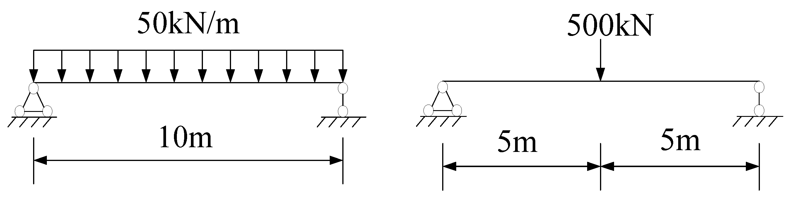
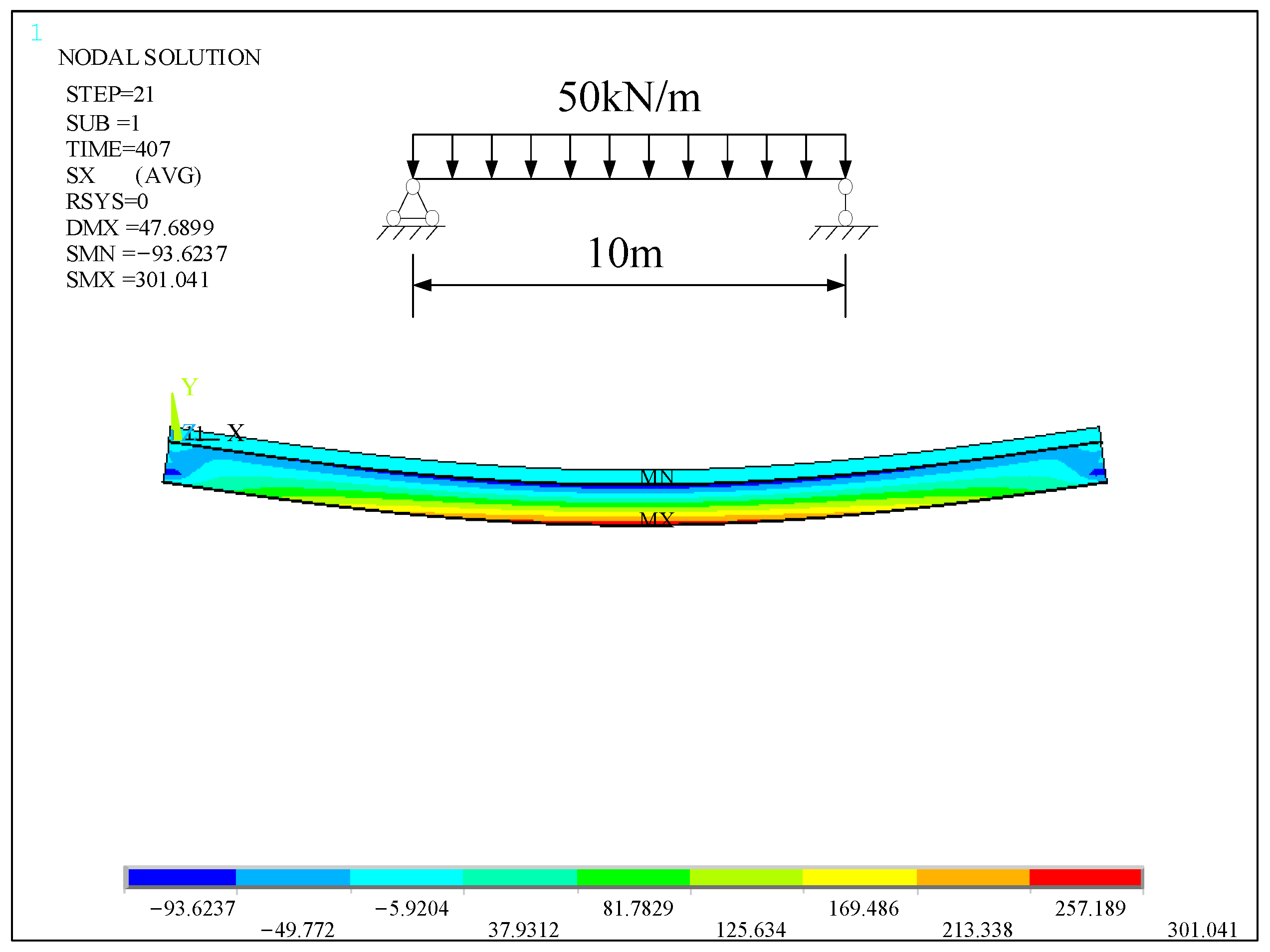
4.1. Example Model

The specific section size and parameters of the composite beam are shown in Figure 6 below. The span of the simply-supported beam is 10 m; the concrete slab is C30 concrete, the elastic modulus Ec = 30 GPa, and Poisson’s ratio μ = 0.2. The steel is HPB300, elastic modulus Es = 210 GPa; the average ambient humidity PH = 30%, concrete loading age t₀ = 7 d, every 20 d to calculate the concrete creep coefficient at dt = 20 d, a total of 407 d. The calculated stiffness of a 19-mm-diameter stud commonly used in engineering is 52,396 N/mm, as calculated by the Chinese Structural Steel Design Code. For ease of calculation, this paper selects the calculated stiffness of stud connectors K = 5 × 10⁴ N/mm, stud spacing e = 100 mm, as shown in Figure 7.

Figure 8 shows a schematic diagram of the composite beam under uniform and concentrated loads. The span of the simply-supported composite beam is 10 m, the uniform load is 50 kN/m, and the concentrated load is 500 kN.

Figure 9 shows the time-varying creep coefficient obtained by using the calculation method of the creep coefficient in China’s Code for Design of Highway Reinforced Concrete and Prestressed Concrete Bridges and Culverts.

Figure 10 is the modeling graph obtained in the ANSYS software. Due to the symmetry of the structural load, a 1/2 structure is adopted to reduce the calculation amount. In the ANSYS output results, the deflection and slip are equivalent to the original structure, and the axial force needs to be multiplied by two times the coefficient.

Figure 11 and Figure 12 are the stress nephograms of the simply-supported composite beam on the 0th day and 407th day under a uniform load, respectively. It can be clearly seen from the diagram that the stress at the mid-span of the simply-supported composite beam is the largest. The maximum stress in the mid-span on the 0th day is 255.551 MPa, and the maximum stress on the 407th day increases to 301.041 MPa, an increase of 17.8%.

Figure 13 and Figure 14 are the stress nephograms of the simply-supported composite beam on the 0th day and 407th day under a concentrated load, respectively. It can be clearly seen from the diagram that the stress at the mid-span of the simply-supported composite beam is the largest. The maximum stress in the mid-span on the 0th day is 510.813 MPa, and the maximum stress on the 407th day increases to 603.365 MPa, an increase of 18.1%.

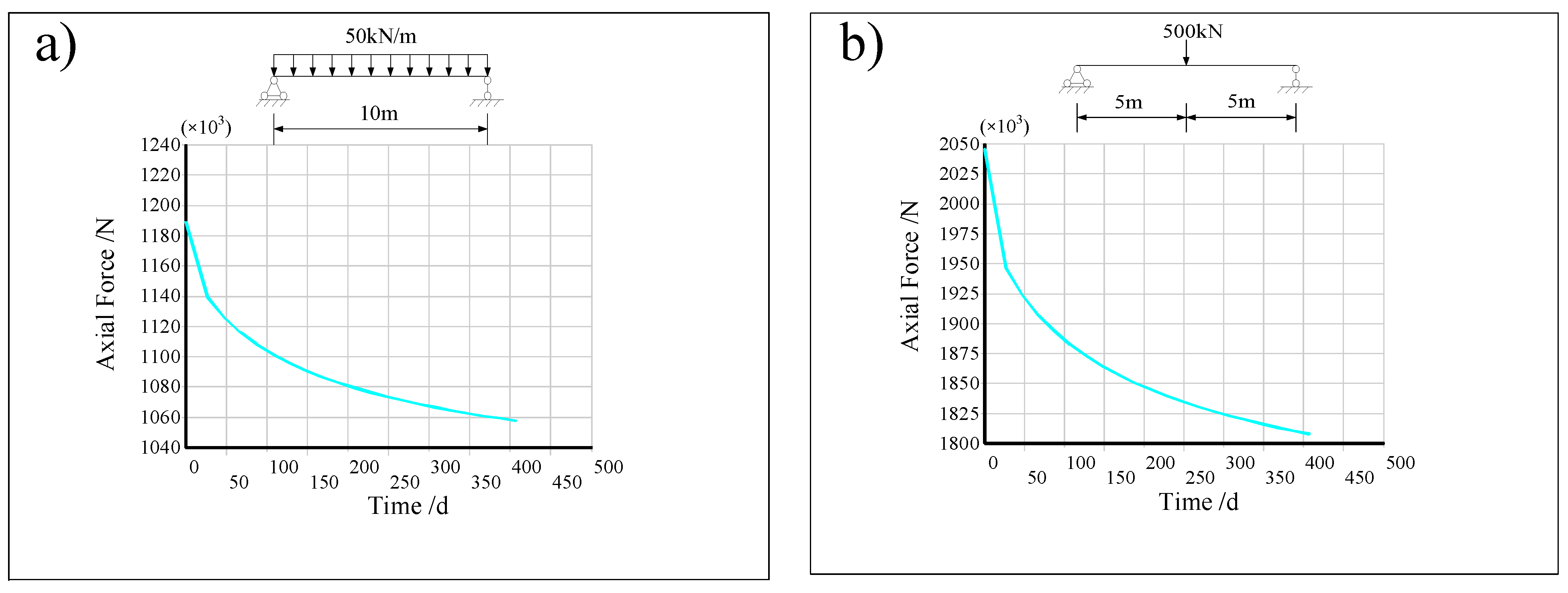
4.2. Comparison of Axial Force under Different Load Situations

The comparative analysis of axial force mainly analyzes the axial force of the concrete slab and steel beam. We take the axial force at the mid-span section for the comparative analysis. Due to the structural balance, it can be seen that the axial forces of the concrete slab and steel beam are equal but opposite.

In

Table 1. Comparison of axial forces under different loads (kN).

Time/d	Simulated Calculation Value		Values Calculated		Error 1	Error 2
	Uniformly Distributed Load	Point Load	Uniformly Distributed Load	Point Load
7	1189.13	2045.54	1189.85	2045.45	0.06%	0.00%
27	1139.33	1953.53	1146.99	1988.02	0.67%	2.09%
47	1126.02	1929.50	1130.03	1960.89	0.35%	1.89%
67	1116.20	1911.73	1118.80	1942.76	0.23%	1.83%
87	1108.33	1897.53	1110.37	1929.11	0.18%	1.82%
107	1101.76	1885.73	1103.64	1918.20	0.17%	1.85%
127	1096.15	1875.69	1098.09	1909.15	0.18%	1.88%
147	1091.27	1866.97	1093.37	1901.47	0.19%	1.92%
167	1086.96	1859.32	1089.30	1894.83	0.21%	1.97%
187	1083.13	1852.68	1085.73	1889.01	0.24%	2.01%
207	1079.69	1846.55	1082.58	1883.85	0.27%	2.05%
227	1076.57	1841.03	1079.75	1879.23	0.29%	2.10%
247	1073.74	1836.01	1077.21	1875.06	0.32%	2.14%
267	1071.15	1831.42	1074.90	1871.29	0.35%	2.17%
287	1068.77	1827.22	1072.80	1867.84	0.38%	2.21%
307	1066.57	1823.34	1070.87	1864.68	0.40%	2.25%
327	1064.53	1819.75	1069.09	1861.77	0.43%	2.27%
347	1062.72	1816.42	1067.45	1859.08	0.44%	2.31%
367	1060.96	1813.33	1065.93	1856.59	0.47%	2.34%
387	1059.30	1810.43	1064.51	1854.27	0.49%	2.37%
407	1057.76	1807.72	1063.19	1852.10	0.51%	2.40%

Note: Error 1 is under uniform load; Error 2 is under concentrated load.

, the axial forces in the span of the combined beam with time for different load forms and different calculation methods are listed.

From the comparison of the axial forces in Table 1, we can clearly see that with increasing time, the axial force of the concrete slab (steel beam) decreases gradually due to the creep effect under both a uniform load and a concentrated load. Comparing the calculated value of the analysis formula with the ANSYS finite element simulation calculation value, we can see that the error between the two increases with time, but the maximum error is only 2.4%.

Figure 15 shows the variation curves of the axial force in the concrete slab of the mid-span section of the composite beam calculated by the ANSYS finite element software, considering the change in creep with time. It can be seen that when the loading age is 7 d under a uniform load, the axial force in the concrete slab (steel beam) is 1189.13 kN, and the axial force is reduced to 1057.76 kN at 407 d, which is reduced by approximately 11 %. When the loading age is 7 d under a concentrated load, the axial force in the concrete slab (steel beam) is 2045.54 kN, and the axial force is reduced to 1807.72 kN at 407 d, which is reduced by approximately 11.6%.

Figure 16 shows the curves of the axial force in the concrete slab of the composite beam’s mid-span section, considering the change in creep with time, calculated using the formula derived by the MATLAB software. It can be seen that when the loading age is 7 d under a uniform load, the axial force in the concrete slab (steel beam) is 1189.85 kN, and the axial force is reduced to 1063.19 kN at 407 d, which is reduced by approximately 10.6 %. When the loading age is 7 d under a concentrated load, the axial force in the concrete slab (steel beam) is 2045.45 kN, and the axial force is reduced to 1852.10 kN at 407 d, which is reduced by approximately 9.45%.

Figure 17 compares the axial force curves in the concrete slab under the two methods. From the diagram, the trend of the curves calculated by the two methods is the same, and the curves of the two methods coincide in the case of a uniform load. In the case of a concentrated load, the curve’s trend is the same, but there are some minor errors. The error range is within 2.4% from the above table.

It can be seen that the formula for calculating the internal axial force of composite beams considering creep and slip coupling derived in this paper is basically consistent with the results obtained by the ANSYS finite element software simulation, which proves the correctness of the derivation results and finite element simulation.

4.3. Comparison of Deflection under Different Load Situations

Due to the simply-supported beam that we selected, for the comparative deflection analysis, we selected the maximum deflection—that is, the mid-span analysis—and could observe the influence of slip and creep on the deflection.

In

Table 2. Comparison of deflection under different loads (mm).

Time/d	Simulated Calculation Value		Values Calculated		Error 1	Error 2
	Uniformly Distributed Load	Point Load	Uniformly Distributed Load	Point Load
7	31.5	50.86	31.11	50.38	1.24%	0.95%
27	38.62	61.86	37.50	60.62	2.98%	2.05%
47	39.95	63.96	38.55	62.28	3.64%	2.70%
67	40.78	65.27	39.20	63.31	4.04%	3.10%
87	41.38	66.22	39.67	64.06	4.31%	3.37%
107	41.84	66.96	40.04	64.65	4.50%	3.58%
127	42.22	67.56	40.34	65.12	4.66%	3.74%
147	42.54	68.06	40.59	65.52	4.80%	3.87%
167	42.81	68.49	40.81	65.87	4.90%	3.98%
187	43.05	68.86	41.00	66.17	5.01%	4.07%
207	43.26	69.19	41.16	66.43	5.10%	4.16%
227	43.44	69.48	41.31	66.66	5.16%	4.23%
247	43.61	69.75	41.44	66.87	5.24%	4.31%
267	43.76	69.98	41.56	67.06	5.30%	4.36%
287	43.89	70.2	41.67	67.23	5.33%	4.42%
307	44.02	70.39	41.77	67.39	5.40%	4.46%
327	44.13	70.57	41.86	67.53	5.43%	4.50%
347	44.23	70.73	41.94	67.66	5.46%	4.53%
367	44.33	70.89	42.02	67.79	5.50%	4.58%
387	44.42	71.03	42.09	67.90	5.54%	4.61%
407	44.51	71.16	42.16	68.01	5.58%	4.64%

Note: Error 1 is under uniform load; Error 2 is under concentrated load.

, the spanwise deflections of the combined beams with time for different load forms and different calculation methods are listed.

From Table 2, we can see that with increasing time, considering the change in the slip effect with time, the deflection of the mid-span section of the composite beam gradually increases. The difference between the results calculated by the two methods under uniform and concentrated loads is 5.58%.

Figure 18 shows the deflection curves of the mid-span section of the composite beam considering the creep change with time calculated in the ANSYS finite element software. It can be seen that when the loading age is 7 d under a uniform load, the mid-span deflection of the composite beam is 31.5 mm, and the deflection increases to 44.51 mm at 407 d, an increase of approximately 41.3%. When the loading age is 7 d under a concentrated load, the mid-span deflection of the composite beam is 50.86 mm, and the deflection increases to 71.16 mm at 407 d, an increase of approximately 39.91%.

Figure 19 shows the deflection curves of the mid-span section of the composite beam considering the change in creep with time calculated by the formula derived by the MATLAB software. It can be seen that when the loading age is 7 d under a uniform load, the deflection of the composite beam is 31.11 mm, and the deflection increases to 42.16 mm at 407 d, an increase of approximately 35.5 %. When the loading age is 7 d under a concentrated load, the deflection of the composite beam is 50.38 mm, and the deflection increases to 68.01 mm at 407 d, an increase of approximately 34.99 %.

Figure 20 shows the comparison of the deflection curves of the mid-span section of the composite beam under the two methods. It can be clearly seen from the figure that the trends of the curves calculated by the two methods under a uniform load and concentrated load are the same, but there are some minor errors. The error range is within 5.58% from the above table.

It can be seen that the formula for calculating the deflection of composite beams considering creep and slip coupling is also basically consistent with the results obtained by the ANSYS finite element software simulation.

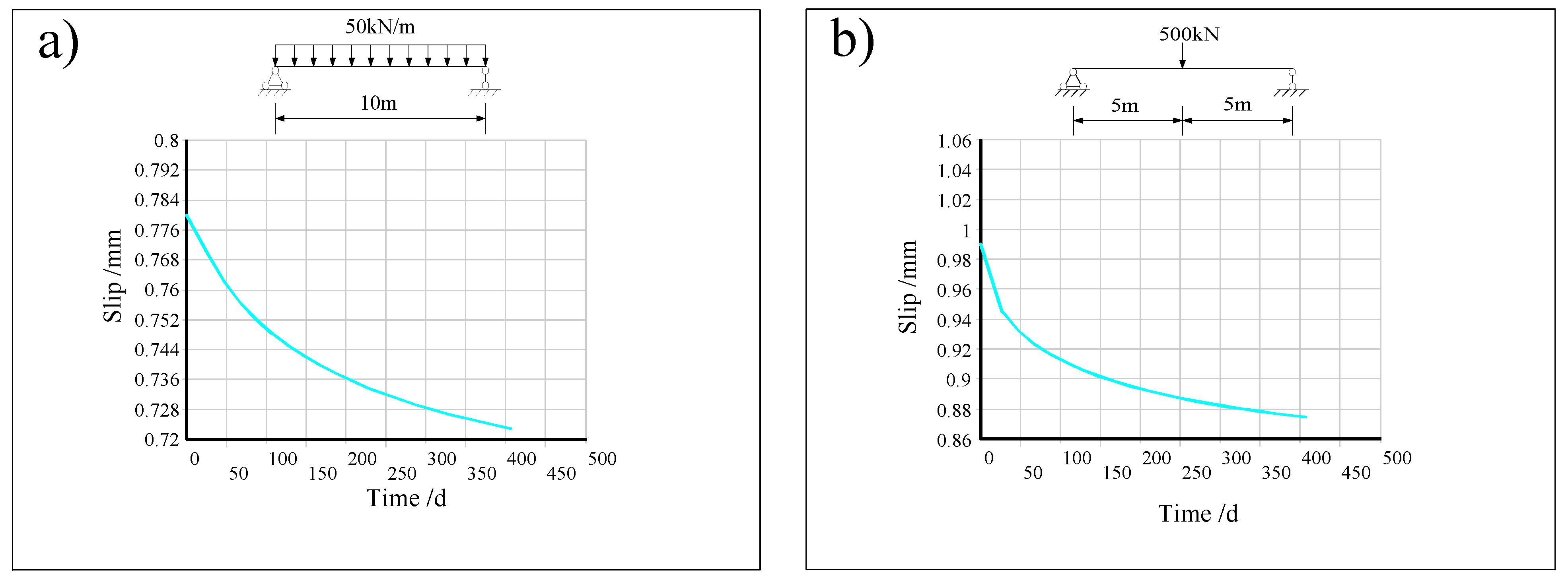
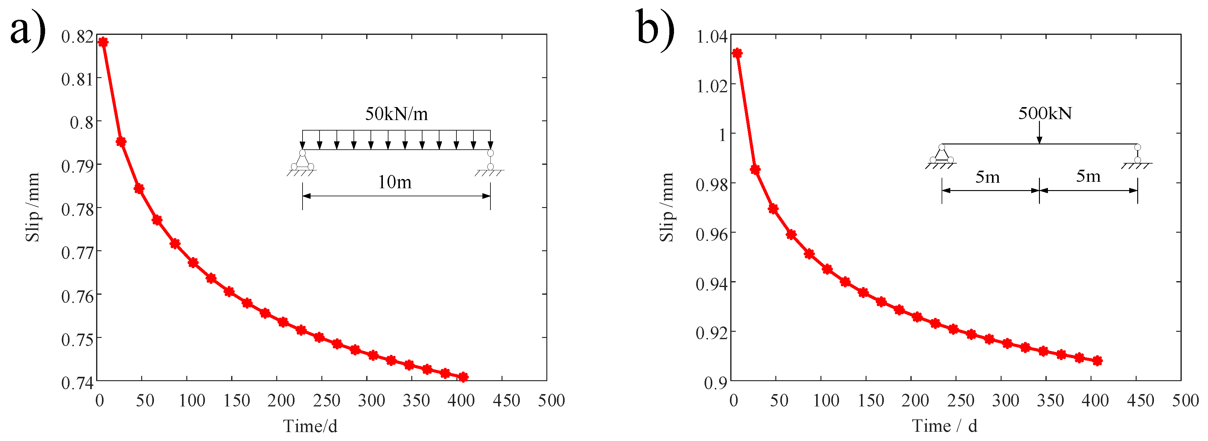
4.4. Comparison of Slip under Different Load Situations

Since the slip at the end of the support is the largest among the simply-supported composite beams, we compare the slip at the end of the composite beam with the time.

In

Table 3. Comparison of slip under different loads (mm).

Time/d	Simulated Calculation Value		Simulated Calculation Value		Error 1	Error 2
	Uniformly Distributed Load	Point Load	Uniformly Distributed Load	Point Load
7	0.7800	0.9901	0.8182	1.0323	4.67%	4.09%
27	0.7696	0.9450	0.7952	0.9853	3.22%	4.09%
47	0.7622	0.9324	0.7844	0.9695	2.82%	3.82%
67	0.7567	0.9236	0.7771	0.9591	2.63%	3.70%
87	0.7522	0.9167	0.7716	0.9513	2.52%	3.63%
107	0.7484	0.9110	0.7673	0.9451	2.46%	3.61%
127	0.7452	0.9062	0.7637	0.9400	2.42%	3.59%
147	0.7424	0.9021	0.7606	0.9356	2.39%	3.58%
167	0.7399	0.8985	0.7579	0.9319	2.38%	3.58%
187	0.7376	0.8953	0.7556	0.9286	2.38%	3.59%
207	0.7356	0.8925	0.7535	0.9258	2.38%	3.59%
227	0.7338	0.8899	0.7517	0.9232	2.38%	3.60%
247	0.7322	0.8876	0.7500	0.9208	2.38%	3.61%
267	0.7307	0.8855	0.7485	0.9187	2.38%	3.62%
287	0.7293	0.8835	0.7471	0.9168	2.39%	3.63%
307	0.7280	0.8817	0.7459	0.9151	2.40%	3.65%
327	0.7269	0.8802	0.7447	0.9134	2.39%	3.64%
347	0.7258	0.8786	0.7436	0.9120	2.40%	3.66%
367	0.7248	0.8772	0.7426	0.9106	2.40%	3.66%
387	0.7238	0.8759	0.7417	0.9093	2.41%	3.67%
407	0.7229	0.8746	0.7408	0.9081	2.42%	3.69%

Note: Error 1 is under uniform load; Error 2 is under concentrated load.

, the beam end slips of the combined beam with time for different load forms and different calculation methods are listed.

Table 3 shows that the slip at the end of the composite beam decreases with time, whether under a uniform or concentrated load. The maximum error between the calculated value of the formula and the simulated value is 4.67%.

Figure 21 shows the curves of the slip size of the composite beam end calculated in the ANSYS finite element software, considering the creep change with time. It can be seen that when the loading age is 7 d under a uniform load, the end slip of the composite beam is 0.7800 mm, and the slip is reduced to 0.7229 mm at 407 d, which is reduced by approximately 7.32%. When the loading age is 7 d under a concentrated load, the end slip of the composite beam is 0.9901 mm, and the slip is reduced to 0.8746 mm at 407 d, which is reduced by approximately 11.67%.

Figure 22 shows the curves of the slip size of the composite beam end considering the change in creep with time calculated by the formula derived by the MATLAB software. It can be seen that when the loading age is 7 d under a uniform load, the slip of the composite beam end is 0.8182 mm, and the slip decreases to 0.7408 mm at 407 d, which is reduced by approximately 9.46%. When the loading age is 7 d under a concentrated load, the slip of the composite beam end is 1.0323 mm, and the slip decreases to 0.9081 mm at 407 d, which is reduced by approximately 12.03%.

Figure 23 shows the comparison of the slip curves of the composite beam end under the two methods. From the diagram, we can clearly see that the trend of the curves calculated by the two methods is the same, whether under a uniform load or concentrated load, but there are some minor errors. The error range is within 4.67% from the above table.

4.5. Comparison of Axial Force, Deflection, and Slip of Composite Beams under Different Stud Stiffness Levels

With the remaining factors of the example model unchanged, the stud stiffness is changed to $K_1=2\times {10}^{4}N/\mathrm{mm}$, $K_2=5\times {10}^{4}N/\mathrm{mm}$ and $K_3=1\times {10}^{5}N/\mathrm{mm}$. The change in stud stiffness causes a change in interface slip between the composite beams. At this time, the changes in the axial force, deflection, and slip of composite beams with different stud stiffness levels under a uniform load are analyzed.

In

Table 4. Comparison of axial force of composite beams with different stud stiffnesses (kN).

Time/d	Simulated Calculation Value			Values Calculated			Error 1	Error 2	Error 3
	${\mathit{K}}_1=2\times {10}^4$ $\mathbf{N}/\mathrm{mm}$	${\mathit{K}}_2=5\times {10}^4$ $\mathbf{N}/\mathrm{mm}$	${\mathit{K}}_3=1\times {10}^5$ $\mathbf{N}/\mathrm{mm}$	${\mathit{K}}_1=2\times {10}^4$ $\mathbf{N}/\mathrm{mm}$	${\mathit{K}}_2=5\times {10}^4$ $\mathbf{N}/\mathrm{mm}$	${\mathit{K}}_3=1\times {10}^5$ $\mathbf{N}/\mathrm{mm}$
7	1023.35	1189.13	1254.24	1024.12	1189.85	1254.84	0.08%	0.06%	0.05%
407	950.79	1057.76	1097.51	949.62	1063.19	1105.25	0.12%	0.51%	0.71%
value	−72.56	−131.37	−156.73	−74.5	−126.66	−149.59

Note: Error 1: between numerical solution and formula solution under stiffness of studs $K_1$; Error 2: between numerical solution and formula solution under stiffness of studs $K_2$; Error 3: between numerical solution and formula solution under stiffness of studs $K_3$.

, the axial forces in the span of the combined beam at day 7 and day 407 of loading are listed for different stud stiffnesses and different calculation methods.

Table 4 shows that regardless of the type of stud stiffness, the maximum error between the calculated value and the numerical simulation value is 0.71%. With the increase in stud stiffness, the axial force decreases more in the same creep time under the formula calculation results, which are 72.56 kN, 131.37 kN, 156.73 kN, respectively. The change rate is 7.09%, 11.05%, and 12.50%.

In

Table 5. Comparison of deflection of composite beams with different stud stiffnesses (mm).

Time/d	Simulated Calculation Value			Values Calculated			Error 1	Error 2	Error 3
	${\mathit{K}}_1=2\times {10}^4$ $\mathbf{N}/\mathrm{mm}$	${\mathit{K}}_2=5\times {10}^4$ $\mathbf{N}/\mathrm{mm}$	${\mathit{K}}_3=1\times {10}^5$ $\mathbf{N}/\mathrm{mm}$	${\mathit{K}}_1=2\times {10}^4$ $\mathbf{N}/\mathrm{mm}$	${\mathit{K}}_2=5\times {10}^4$ $\mathbf{N}/\mathrm{mm}$	${\mathit{K}}_3=1\times {10}^5$ $\mathbf{N}/\mathrm{mm}$
7	37.29	31.50	29.12	36.91	31.11	28.73	1.02%	1.24%	1.34%
407	49.21	44.51	42.69	46.97	42.16	40.28	4.55%	5.28%	5.65%
value	11.92	13.01	13.57	10.06	11.05	11.55

Note: Error 1: between numerical solution and formula solution under stiffness of studs $K_1$; Error 2: between numerical solution and formula solution under stiffness of studs $K_2$; Error 3: between numerical solution and formula solution under stiffness of studs $K_3$.

, the span deflections of the combined beam at day 7 and day 407 of loading are presented for different stud stiffnesses and different calculation methods.

Table 5 shows that regardless of the stud stiffness, the maximum error between the calculated and numerical simulation values is 5.65%. With the increase in stud stiffness, the deflection increases more in the same creep time under the formula calculation results, which are 11.92 mm, 13.01 mm, and 13.57 mm, respectively. The change rate is 31.97%, 41.30%, and 46.60%.

In

Table 6. Comparison of slip of composite beams with different stud stiffnesses (mm).

Time/d	Simulated Calculation Value			Values Calculated			Error 1	Error 2	Error 3
	${\mathit{K}}_1=2\times {10}^4$ $\mathbf{N}/\mathrm{mm}$	${\mathit{K}}_2=5\times {10}^4$ $\mathbf{N}/\mathrm{mm}$	${\mathit{K}}_3=1\times {10}^5$ $\mathbf{N}/\mathrm{mm}$	${\mathit{K}}_1=2\times {10}^4$ $\mathbf{N}/\mathrm{mm}$	${\mathit{K}}_2=5\times {10}^4$ $\mathbf{N}/\mathrm{mm}$	${\mathit{K}}_3=1\times {10}^5$ $\mathbf{N}/\mathrm{mm}$
7	1.6644	0.7800	0.4290	1.7038	0.8182	0.4442	2.37%	4.90%	3.54%
407	1.5836	0.7229	0.3841	1.5959	0.7408	0.3964	0.78%	2.48%	3.20%
value	−0.0808	−0.0571	−0.0249	−0.1079	−0.0774	−0.0478

Note: Error 1: between numerical solution and formula solution under stiffness of studs $K_1$; Error 2: between numerical solution and formula solution under stiffness of studs $K_2$; Error 3: between numerical solution and formula solution under stiffness of studs $K_3$.

, the beam end slips are listed for different stud stiffnesses and different calculation methods at 7 d and 407 d of loading are presented.

As can be seen from Table 6, the maximum error between the calculated and numerically simulated values is 4.90%, regardless of the stud stiffness. With the increase in the stud stiffness, the decrease in the slip of the equation calculated for the same creep time is smaller, at 0.0808 mm, 0.0571 mm, and 0.0249 mm, respectively, and the rate of change is 4.85%, 7.32%, and 10.47%.

In summary, the existence of slip and creep in composite beams significantly affects the axial force, deflection, and slip of composite beams. The formula solution derived in this paper is basically consistent with the finite element simulation value and is suitable for the solution under different creep and slip effects.

5. Conclusions

• When considering the creep effect of the combined beam at the same stud stiffness, the axial force of the concrete slab inside the combined beam was reduced by around 11.0–11.6%, and the slip was reduced by 7.32–11.67% at 407 d. However, the deflection of the combined beam increased by 39.91–41.3%, so the concrete creep effect reduces the flexural stiffness of the combined structure, increases the deformation of the combined beam, and adversely affects the combined structure.
• The stud stiffness is an important factor affecting the long-term performance of steel–concrete composite beams. The stud stiffness was varied from 2000 N/mm to 10,000 N/mm, with other parameters unchanged. The change in axial force in the combined beam due to creep variation increased from 7.09% to 12.50%; the change in deflection increased from 31.97% to 46.60%, and the change in slip increased from 4.85% to 10.47% under long-term loading. The results show that the more strongly the studs constrain the concrete slab, the greater the adverse effect of concrete creep on the combined beam.
• By comparing the theoretically derived formulation with the finite element numerical simulation results, the error was around 5%, which proves the validity of the formulation for the calculation of the axial force, deflection, and slip of simply-supported composite beams considering the coupling of creep and slip based on the principle of the energy variational method. The results show that the theoretically derived formulas are applicable to the solution of the axial force, deflection, and slip of simply-supported composite beams under different types of creep and slip coupling.

References

1. Xiao, L.; Wei, X.; Wen, Z.; Li, G. State-of-the-art review of steel-concrete composite bridges in 2019. J. Civ. Environ. Eng. 2020, 42, 168–182. (In Chinese) [Google Scholar]
2. Newmark, N.M.; Siess, C.P.; Viest, I.M. Tests and analysis of composite beams with incomplete interaction. Proc. Soc. Exp. Stress Anal. 1951, 9, 75–92. [Google Scholar]
3. Adekola, A.O. The dependence of shear lag on partial interaction in composite beams. Int. J. Solids. Struct. 1974, 10, 389–400. [Google Scholar] [CrossRef]
4. Girhammar, U.A.; Pan, D. Dynamic analysis of composite members with interlayer slip. Int. J. Solids. Struct. 1993, 30, 797–823. [Google Scholar] [CrossRef]
5. Oehlers, D.J.; George, S. Composite Beams with Limited-Slip-Capacity Shear Connectors. J. Struct. Eng. 1995, 121, 932–938. [Google Scholar] [CrossRef]
6. Fabbrocino, G.; Manfredi, G.; Cosenza, E. Nonlinear analysis of composite beams under positive bending. Comput. Struct. 1999, 70, 77–89. [Google Scholar] [CrossRef]
7. Tarantino, A.M.; Dezi, L. Creep effects in composite beam s with flexible shear connectors. J. Struct. Eng. ASCE 1992, 118, 2063–2080. [Google Scholar] [CrossRef]
8. Dezi, L.; Tarantino, A.M. Creep in composite continuous beams. I: Theoretical treatment. J. Struct. Eng. 1993, 119, 2095–2111. [Google Scholar] [CrossRef]
9. Dezi, L.; Tarantino, A.M. Creep in composite continuous beams. II: Parametric study. J. Struct. Eng. 1993, 119, 2112–2133. [Google Scholar] [CrossRef]
10. Gilbert, R.I.; Bradford, M.A. Time-dependent behavior of continuous composite beams at service loads. J. Struct. Eng. 1995, 121, 319–327. [Google Scholar] [CrossRef]
11. Dezi, L.; Leoni, G.; Tarantino, A.M. Time-dependent analysis of prestressed composite beams. J. Struct. Eng. 1995, 121, 621–633. [Google Scholar] [CrossRef]
12. Dezi, L.; Leoni, G.; Tarantino, A.M. Algebraic method for creep analysis of continuous composite beams. J. Struct. Eng. 1996, 122, 423–430. [Google Scholar] [CrossRef]
13. Amadio, C.; Fragiacomo, M. Simplified approach to evaluate creep and shrinkage effects in steel-concrete composite beams. J. Struct. Eng. 1997, 123, 1153–1162. [Google Scholar] [CrossRef]
14. Nie, J. Calculation and analysis of long-term deformation of steel-concrete composite beams. Build. Struct. 1997, 1, 42–45. (In Chinese) [Google Scholar] [CrossRef]
15. Dezi, L. Time-dependent analysis of shear-lag effect in composite beams. J. Eng. Mech. 2001, 127, 71–79. [Google Scholar] [CrossRef]
16. Zhou, L. The stress redistribution in steel-concrete composite girders due to shrinkage and creep of concrete. Bridge Constr. 2001, 2, 1–4. (In Chinese) [Google Scholar]
17. Sheng, X.; Yang, J. Redistribution of creep stress in prestressed concrete build-up beam. Bridge Constr. 2003, 4, 11–14. (In Chinese) [Google Scholar]
18. Nie, J.; Cai, C. Steel–concrete composite beams considering shear slip effects. J. Struct. Eng. 2003, 129, 495–506. (In Chinese) [Google Scholar] [CrossRef] [Green Version]
19. Jiang, L.; Yu, Z.; Li, J. Theoretical analysis of slip and deformation of steel-concrete composite beam under uniform distributed loads. Eng. Mech. 2003, 2, 133–137. (In Chinese) [Google Scholar]
20. Wang, J.; Long, P.; Liu, Z. Analysis of creep in composite beams. Highw. Traffic Sci. Technol. 2004, 8, 38–41. (In Chinese) [Google Scholar]
21. Qiu, W.; Jiang, M.; Zhang, Z. Finite element analysis for creep and shrinkage of steel-concrete composite beams. Eng. Mech. 2004, 4, 162–166. (In Chinese) [Google Scholar]
22. Fan, J.; Nie, J.; Wang, H. Long-term behavior of composite beams with shrinkage, creep and cracking (I)–Experiment and calculation. China. Civ. Eng. J. 2009, 42, 8–15. (In Chinese) [Google Scholar]
23. Fan, J.; Nie, X.; Li, Q. Long-term behavior of composite beams with shrinkage, creep and cracking (II)–theoretical analysis. China. Civ. Eng. J. 2009, 42, 16–22. (In Chinese) [Google Scholar]
24. Nguyen, Q.H.; Mohammed, H.; Brian, U. Time-dependent analysis of composite beams with continuous shear connection based on a space-exact stiffness matrix. Eng. Struct. 2010, 32, 2902–2911. [Google Scholar] [CrossRef]
25. Nguyen, Q.H.; Mohammed, H. Nonlinear time-dependent behavior of composite steel-concrete beams. J. Struct. Eng. 2016, 142, 04015175. [Google Scholar] [CrossRef]
26. Miao, L.; Chen, D. Closed-form solution of composite beam considering interfacial slip effects. J. Tongji Univ. Nat.Sci. 2011, 39, 1113–1119. (In Chinese) [Google Scholar]
27. Ji, W.; Sun, B.; Deng, L.; Zhao, Y.; Lin, P. Calculation and analysis on deflection of steel-concrete continuous composite girder considering effect of multi-factors. J. Hunan Univ. Nat.Sci. 2019, 46, 30–38. (In Chinese) [Google Scholar]
28. Oven, V.A.; Burgess, I.W.; Plank, R.J. An analytical model for the analysis of composite beams with partial interaction. Comput. Struct. 1997, 62, 493–504. [Google Scholar] [CrossRef]
29. Salari, M.R.; Spacone, E.; Shing, P.B. Nonlinear analysis of composite beams with deformable shear connectors. J. Struct. Eng. 1998, 124, 1148–1158. [Google Scholar] [CrossRef]
30. Gattesco, N. Analytical modeling of nonlinear behavior of composite beams with deformable connection. J. Constr. Steel. Res. 1999, 52, 195–218. [Google Scholar] [CrossRef]
31. Ayoub, A.; Filippou, F.C. Mixed formulation of nonlinear steel-concrete composite beam element. J. Struct. Eng. 2000, 126, 371–381. [Google Scholar] [CrossRef]
32. Qiu, W.; Zhang, Z.; Huang, C. Finite-element method of double-layer beam model for analysis of composite steel-concrete beams. J. Dalian Univ. Technol. 2003, 1, 101–103. (In Chinese) [Google Scholar]
33. Fang, K.; Chen, S. Finite element analysis of steel-concrete composite beams with influence of the shear connector stiffness. Ind. Buils. 2003, 9, 75–77. (In Chinese) [Google Scholar]
34. Wei, F.; Lv, Z.; Sun, W. Nonlinear finite element analysis of composite steel-concrete beams with partial shear connection. Ind. Build. 2003, 9, 78–79 + 88. (In Chinese) [Google Scholar]
35. Miranda, M.P.; Tamayo, J.L.P.; Morsch, I.B. Reassessment of viscoelastic response in steel-concrete composite beams. Struct. Eng. Mech. 2022, 81, 617–631. [Google Scholar] [CrossRef]
36. Sarfarazi, V.; Haeri, H.; Shemirani, A.B.; Zhu, Z.; Marji, M.F. Experimental and numerical simulating of the crack separation on the tensile strength of concrete. Struct. Eng. Mech. Int. J. 2018, 66, 569–582. [Google Scholar] [CrossRef]
37. Wang, Q.; Yang, J.; Zhang, Y. Analysis and design of long-term responses of simply-supported steel–concrete composite slabs. J. Build. Eng. 2022, 53, 104496. [Google Scholar] [CrossRef]
38. Huang, Q.; Li, W.; Wang, B. Analytical method of steel-concrete composite beam based on interface slip and shear deformation. J. Nanjing Univ. Aeronaut. Astronaut. 2018, 50, 131–137. (In Chinese) [Google Scholar]
39. JTG 3362-2018; Code for design of highway reinforced concrete and prestressed concrete bridges and culverts. People’s Transportation Publishing House: Beijing, China, 2018. (In Chinese)
40. Liu, Y.; Liu, X. Long-term deflection of steel-concrete composite box-beam due to creep. J. Railw. Sci. Eng. 2015, 12, 317–322. (In Chinese) [Google Scholar]
Figure 1. Composite beam transverse section diagram.
Applsci 13 00193 g001
Figure 2. Longitudinal section diagram of composite beam.
Applsci 13 00193 g002
Figure 3. Shear connection diagram.
Applsci 13 00193 g003
Figure 4. Simply-supported beam under uniform load.
Applsci 13 00193 g004
Figure 5. Simply-supported beam under concentrated load.
Applsci 13 00193 g005
Figure 6. ANSYS finite element model.
Applsci 13 00193 g006
Figure 7. Section size and parameters of composite beam.
Applsci 13 00193 g007
Figure 8. Uniform and concentrated load diagram of composite beam.
Applsci 13 00193 g008
Figure 9. Creep coefficient varying with time.
Applsci 13 00193 g009
Figure 10. ANSYS software modeling diagram.
Applsci 13 00193 g010
Figure 11. The stress cloud diagram of ANSYS under uniform load on day 0.
Applsci 13 00193 g011
Figure 12. The stress cloud diagram of ANSYS under uniform load on day 407.
Applsci 13 00193 g012
Figure 13. The stress cloud diagram of ANSYS under concentrated load on day 0.
Applsci 13 00193 g013
Figure 14. The stress cloud diagram of ANSYS under concentrated load on day 407.
Applsci 13 00193 g014
Figure 15. (a) Mid-span axial force diagram under uniform loads in ANSYS. (b) Mid-span axial force diagram under point loads in ANSYS.
Applsci 13 00193 g015
Figure 16. (a) Mid-span axial diagram under uniform loads in MATLAB. (b) Mid-span axial diagram under point loads in MATLAB.
Applsci 13 00193 g016
Figure 17. (a) Comparison diagram of mid-span axial force under uniform loads. (b) Comparison diagram of mid-span axial force under point loads.
Applsci 13 00193 g017
Figure 18. (a) Mid-span deflection under uniform loads in ANSYS. (b) Mid-span deflection under point loads in ANSYS.
Applsci 13 00193 g018
Figure 19. (a) Mid-span deflection under uniform loads in MATLAB. (b) Mid-span deflection under point loads in MATLAB.
Applsci 13 00193 g019
Figure 20. (a) Comparison diagram of mid-span deflection under uniform loads. (b) Comparison diagram of mid-span deflection under point loads.
Applsci 13 00193 g020
Figure 21. (a) Beam end slip under uniform loads in ANSYS. (b) Beam end slip under different loads in ANSYS.
Applsci 13 00193 g021
Figure 22. (a) Beam end slip under uniform loads in MATLAB. (b) Beam end slip under point loads in MATLAB.
Applsci 13 00193 g022
Figure 23. (a) Comparison of beam end slip under uniform loads. (b) Comparison of beam end slip under point loads.
Applsci 13 00193 g023