1. Introduction
The Roadmap to the Realization of Fusion Energy of the European scientific program [
1,
2] includes driving experiments that aim to support the accomplishment of ITER and prepare the route for the future demonstration fusion power plant DEMO. Both ITER and DEMO are tokamak type reactors. A tokamak device exploits the superimposition of controlled magnetic fields to drive the plasma current to the operative limit and to contain the drift of the confined particles. The plasma is harnessed on torus-helical field lines generated by eighteen (in the case of ITER) or sixteen (for DEMO) Toroidal Field (TF) D-shaped magnets, arranged around the machine central axis; six Poloidal Field (PF) annular coils, which surround the TF coils, and a central transformer named Central Solenoid (CS), placed inside the machine bore. A Tokamak reactor operates under extremely demanding loading conditions, leading the components near to their mechanical limits. Due to the pulsing electromagnetic loads, all structures must be assessed under the static as well as fatigue behavior. This paper focuses on the main studies and calculations completed at the end of the pre-concept design phase of the DEMO system [
3,
4]. As detailed in the following, the assessment has been performed implementing the Finite Element method by defining a parametrical electromagnetic model and a related structural model of the machine, which consist of the three main magnetic systems (TF, PF and CS), the structures, the auxiliary components and the bolted joint connections.
2. DEMO: The Design and the Rationale Behind
The functioning of DEMO, or more in general of a tokamak (“тopoидaльнaя кaмepa в мaгнитныx кaтyшкax”) machine, is based on the interaction of huge magnetic fields. The attainment of the necessary conditions to initiate the fusion reactions is constrained by three parameters: the density of the plasma particles n, the plasma temperature T and the energy confinement time τE. These parameters are intertwined and different relations, as e.g., Lawson’s law, describe the theoretical processes to obtain the fusion reactions, stabilize them and draw energy.
The challenge of the magnetic confinement machines consists in increasing τE by trapping a suspended plasma at a very high temperature (108 K) inside a closed configuration. The elemental closed magnetic configuration is given by a toric solenoid, with poloidally wound coils that generate a toroidal field. The force lines exerted are coaxial and centered on the torus axis, with the toroidal magnetic field decreasing linearly along the radial direction. Each particle linked to the magnetic flux lines is subjected to an orthogonal force, which produces a drift centrifugal acceleration. Unfortunately, this leads to a charge separation within the plasma, which creates an electric field and generates an electromotive force that contributes to the drift of the particles. Therefore, the pure toroidal configuration is not sufficient for the plasma confinement.
In order counteract the drift acceleration, a poloidal field is superimposed to the toroidal one. This additional field has a lower intensity than the toroidal one, but a greater radial gradient so that the resulting magnetic field has toro-helicoidal force lines where the pitch of each helix is greater than the torus radius, leading the flux lines to close on themselves after some turns around the torus axis.
In a tokamak, the poloidal field is generated by an ideal wire defined by the plasma itself. The plasma is the secondary of a transformer, while the primary circuit is a solenoid placed on the machine central axis. Considering Lentz’s law, the electromagnetic induction is obtained by varying the current on the central circuit. It is important to mention that, since the reverse of the plasma current cannot occur, it is necessary that the magnetic flux and therefore the current vary with a monotonous increasing function, but an infinite current is obviously impossible to achieve. It is therefore necessary to operate the machine in a pulsed regime.
Once this configuration is obtained, the plasma particles, however, tend to expand radially under the action of hydrodynamic forces generated by the current that flows through the plasma itself. Indeed, the particles tend to concatenate the minimum magnetic flux available. This trend is contrasted by introducing a vertical magnetic field interacting with the plasma current by means of external annular coils that surround the toroidal magnets. By properly directing the current in these coils, it is ensured that the resulting action of the hydrodynamic force is directed towards the torus axis.
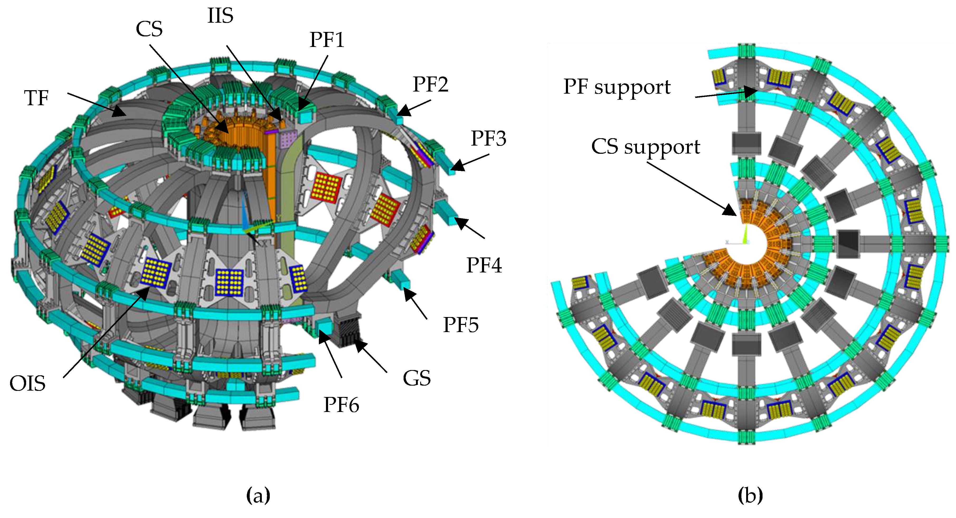
In DEMO, shown in
Figure 1, the toroidal field configuration is obtained with sixteen D-shaped magnets (TF) [
5], the vertical field by six poloidal annular coils (PF) [
6,
7] and the primary transformer circuit by one central solenoid (CS), formed by a stack of five independent modules [
8]. Each magnet system in DEMO includes superconductive coils made of Cable-In-Circuit Conductors (CICC) [
9].
The final function of the poloidal system (CS and PF) consists in driving the plasma current to the operative limits and keeping it stable inside the vessel. One “plasma scenario” has, usually, an early stage first, when the currents of the CS modules vary rapidly to induce the plasma current. Then, in the following time points, a quadrupolar field component counteracts the radial and the vertical expansion of the plasma and produces an ovality of its shape. The subsequent superimposition of a sexto-polar component provides the triangular shape required by the plasma stability.
3. The Electro-Magneto-Mechanical Framework
As mentioned, each plasma pulse is described by the current evolution of each coil over time. The reference scenario scheduled for DEMO [
10] is currently discretized into three time points: (i) premagnetisation (PREMAG); (ii) start of Flattop (SOF) and (iii) end of Flattop (EOF).
Figure 2 and
Figure 3 show the current vs. time in the CS modules and PF coils, respectively, taken from [
10].
Each instant describes a magnet system in equilibrium, where the Lorentz force field is globally balanced in all directions. Considering a cylindrical reference system centered on the machine axis on the equatorial plane, each poloidal coil is subjected to a radial force, which is self-balanced along 360-degrees, and to a positive or negative vertical force, depending on whether the magnets tend to attract or repel each other. The total vertical action given by the poloidal magnets is zero.
From the structural viewpoint, in a tokamak all coils are inter-linked by suitable mechanical systems and fixed to the ground by specific support structures. Two types of systems connect the TF coils one-another: the outer inter-coil structures (OISs) and the inner inter-coil structures (IISs). OISs are located above and below the equatorial ports of the vacuum vessel and form two rings that close the TF assembly and contrast the coils out of plane loads. IISs are located at the top and the bottom of the TF inner straight leg to prevent the de-wedge effect due to eventual outward (i.e., toward the plasma) radial displacements. In normal operation, the overall vertical forces are given by the dead loads only so that the TF connections to the ground are defined “gravity supports” (GSs) [
11]. They are designed to withstand the vertical loads and to exhibit a rather low radial stiffness to follow the shrinking of the machine from room temperature (293 K) to the superconductive coil operating temperature (4.2 K).
Even if the toroidal field is supported by a stationary current in the D-magnets, the mutual interaction with the poloidal system leads the TF system to withstand cyclical loads too. In particular, 20,000 cycles are scheduled for DEMO [
2].
To assess the TF coils and their structures under the fatigue phenomena, for each plasma pulse it necessary to analyse the load conditions causing a stress field in the magnets. To this aim, a total of six representative time points have been considered:
Initial situation with dead weight and pretension of the bolted joint connections.
Cooldown from the room temperature (293 K) to the operating temperature of the superconducting magnets (4.2 K).
Energization of the TF coils (TF ENRG) to the operative current (66 kA) [
5].
Premagnetization (PREMAG).
Start of Flattop (SOF).
End of Flattop (EOF).
The framework of the presented approach consists of two sequentially coupled parts: the electromagnetic section (EMS) and the structural section (SS). In all cases, the governing equations are solved computationally, by means of the finite element method.
EMS is further split two sequentially coupled steps. In the first one, a simple electrostatic study is developed, where voltages are the nodal degree of freedom; the available currents are input as nodal values; proper symmetry conditions are imposed, and the current density distribution is finally calculated. In the second EMS step, a magnetostatic analysis is performed, where the components of the potential are the nodal degree of freedom and the current density distribution previously obtained are exploited as the input data set; symmetry conditions are imposed, and the magnetic field is obtained. The Lorentz force field is finally calculated to feed the structural section.
SS consists of two parts, aimed at the structural assessment and fatigue assessment, respectively. First, a thermomechanical study is carried out. The three components of the displacements and the temperature are the nodal degrees of freedom; proper symmetry and boundary conditions are imposed; the Lorentz forces previously calculated are applied, and the displacement, strain and stress fields are obtained. Given the material heterogeneity, a homogenization procedure is employed to model the TF winding pack as an equivalent orthotropic material (details are given in
Section 5). In the second SS part, described in
Section 6, fatigue is addressed, and the life assessment approach is followed. To this aim, for each finite element, the equivalent alternate fatigue stress is calculated starting from the stress tensor obtained from the previous SS thermomechanical analysis.
4. Electromagnetic Calculation Methodology-EMS Section
To proceed with the structural analysis, it is necessary to complete the magnetic assessment at the main time points of the plasma scenario (PREMAG, SOF and EOF). The final purpose consists of obtaining the Lorentz forces on the toroidal and poloidal coils by means of the electromagnetic model and automatically transferring the loads to the structural environment.
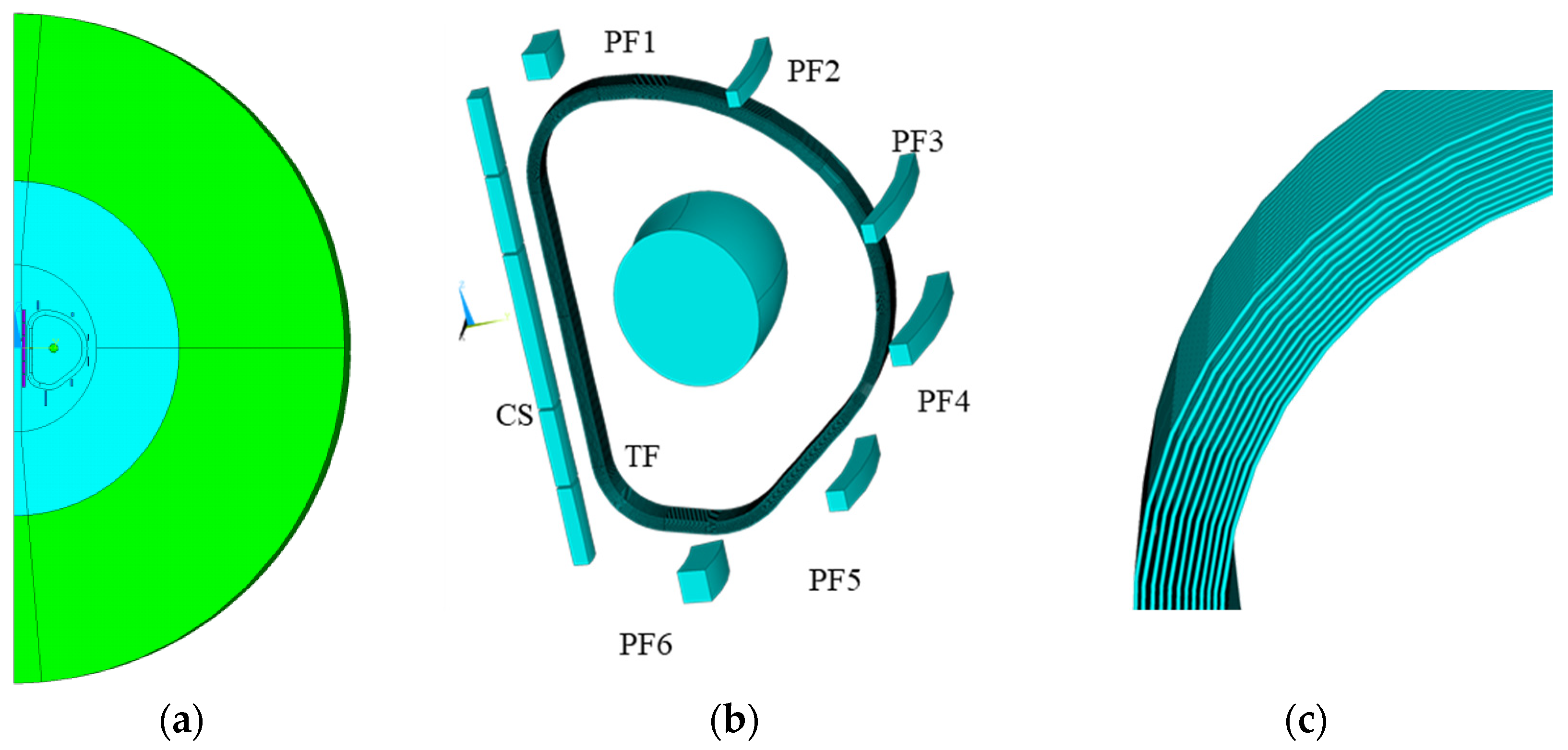
The 3D electromagnetic model is made of the three main DEMO magnet systems and also includes an equivalent coil for an ideal plasma wire, as shown in
Figure 4a,b. The dimensions and positions used to create the magnet domains are taken from [
7,
8]. The geometry is built entirely in the APDL environment of Ansys software, with a parametric script to rapidly deal with changes in the structures and to split the domain into different component sub-domains to be able to produce a mapped mesh. The model is implemented in FORTRAN parametrical language (for a direct usage in Ansys APDL) to have the possibility of defining the coils as an equivalent smeared domain (for the CS and PF coils) as well as a detailed winding system specifying each turn (for the TF coil), as shown in
Figure 4b,c. To this aim, the script starts with a bi-dimensional mesh of the magnet cross-section and then extrudes it along the coil axis. The key idea is to exploit the magnetic discretization for the structural model together with its nodal load information.
For the PF coils and the CS, periodic boundary interfaces are easily identified, as these coils have an axisymmetric geometry. Further, the sixteen TF coils show a 22.5-degree periodicity around the machine axis. Additionally, since one TF coil is completely included inside the repetitive sector considered, a cutting plane is needed to identify the boundary interfaces for this magnet. The TF was therefore trimmed on the equatorial plane, thus obtaining two open circuits with separated but coincident nodes on the cutting plane. By applying mirrored boundary conditions, it is possible to create a continuous current distribution.
As described, the analysis is organized in two steps:
The first step is the electrostatic analysis. The current at the ith time point of the scenario is applied as a nodal value by selecting one of the two periodic boundary faces of each magnet. The correspondent periodic face of each magnet is placed at zero potential. To this aim, eight-node 3D linear solid elements are used, with 1 dof per node (voltage), which can calculate the current density distribution inside the magnet sections. For the magnets modelled as smeared domains (CS and PF), to obtain a constant current density distribution on the coil cross-sections, the resistivity of each element is defined as a material property linearly variable as a function of the radial position. It is important to underline that, if this material property were not properly defined by this linear function, the current density would record an increase from the inner to the outer radius of the coil, thus producing a wrong electromagnetic force field. For the TF coil, modelled detailing its winding pack, each single cable can be assigned a constant resistivity, and no linear function is needed. The cable heterogeneity can be neglected. An example of the current density distribution obtained is shown in
Figure 5.
The second step is the magnetostatic analysis. The input data for the calculation are given by the current density distributions previously obtained. The previous discretization is exploited, made of eight-node 3D linear solid elements. The magnetic vector potential formulation is implemented; therefore, the three components of the potential are the nodal degrees of freedom. For the air domain (
Figure 4a), needed to ensure the correct closure of the flux lines, infinite elements [
12] are used to surround the magnets. The resulting magnetic field is reported in
Figure 6, for the reference time points of the scenario. By means of this model, the Lorentz forces are computed as nodal forces for each magnet.
Focusing on the TF system, it is useful to consider the distribution of the electromagnetic force and moment components along the curvilinear abscissa of the D-shaped magnet, shown
Figure 7 with reference to a cylindrical coordinate system, where
x is the azimuth;
y is the radial distance, and
z is the axial coordinate (height).
Figure 7a shows that the radial component exhibits an intense centripetal action (i.e., toward the machine axis) along the inner leg and the adjacent curved region, while on the outer leg the radial action becomes centrifugal (positive values on the graph). The vertical component of the Lorentz force shows a nearly symmetrical top-down trend; the vertical force rises in the straight part joining the two lower curved sectors (
Figure 7b). These two components are generated and influenced only by the magnetic field produced by the toroidal system. The toroidal (out-of-plane) component is due to the interaction of the TF current with the magnetic field generated by the poloidal system, which varies with the time (
Figure 7c). The same variation is highlighted also on the plots of the moments around the radial and the vertical axes, shown in
Figure 7d,e, respectively. It is worth underlining that, within the TF system, the total moment around the machine vertical axis is zero. Finally,
Figure 7f shows that the most severe action is exercised by the out of plane (OOP) moment, which does not change during the scenario, being composed of the constant components of the force. The effect of the rotation around the OOP axis is balanced by the reactions at the gravity supports and by the contact forces on the inner leg TF cases, where the D-shaped magnets are wedged.
5. Structural Calculation Methodology-Thermomechanical Analysis
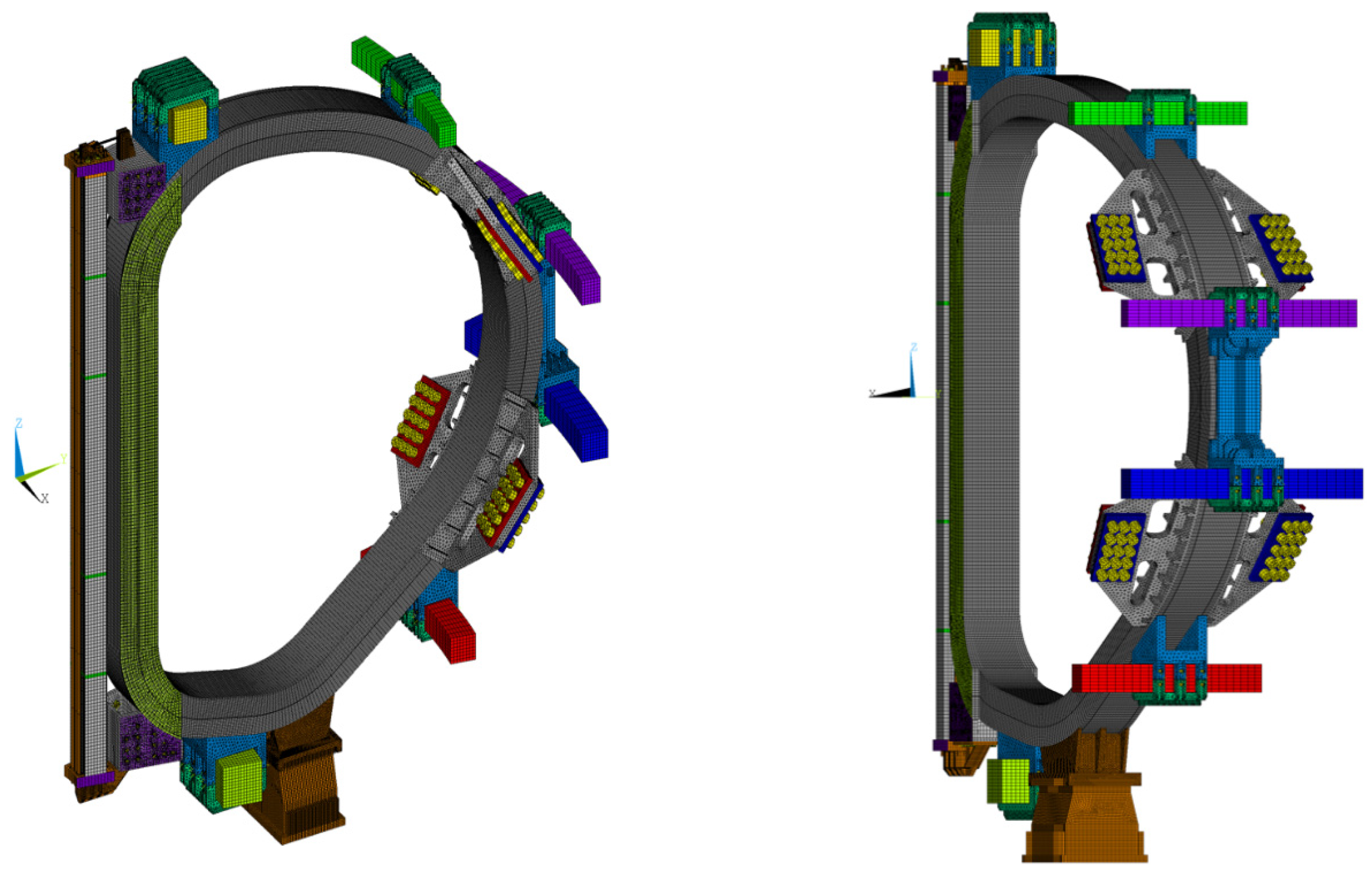
The 3D structural model is shown in
Figure 8. It is made of 3D 8-node (hexahedral) and 4-node (tetrahedral) linear element, with 4 degrees of freedom per node (three translations and the temperature). The structural mesh comprises 1,529,209 elements with 96% of 3D hexahedral elements and only 4% of 3D tetrahedral elements. Actually, as it is easily seen in
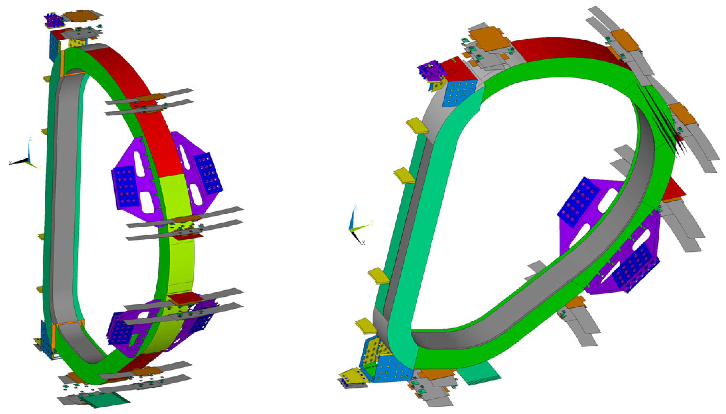
Figure 8, beside the three orders of magnets (inherited from the electromagnetic analysis); the model comprises the main structural elements with several details. As briefly mentioned above, there are two types of inter-coils structures, linking together the TF coils: the outer inter-coil structures (OISs) and the inner inter-coil structures (IISs). The outer inter-coil structures are organized in two orders, located in the curved outer part of the TF case, one above the equatorial plane and the other below. The main function of the OISs is to balance the out-of-plane forces acting on each D-shape coil. They are designed according to the double shear joint scheme and are composed of large-shaped plates rigidly connected to the TF case and bolted to each other on the other side by means of pairs of cover plates. Like ITER, DEMO also relies on the wedging effect to balance the radial forces acting on the inner leg of the TF coils. To prevent the possible detachment and to increase the wedging mechanism, the inner inter-coil structures are located at the ends of the straight leg of each TF coil, one at the top and the other at the bottom. They are of a box-type structure, bolted to each other on both sides in order to provide a very rigid connecting system. Finally, the CS module stack is enclosed inside a preload system capable to withstand the huge repulsion between the modules; the six PF coils are closed inside a dedicated support that counteracts the coil axial movements and allows the radial shrinking; the central solenoid is connected to the bottom end of the inner TF leg by means of a suitable cantilever connection, and the gravity support is modelled in detail.
Each component is connected via mechanical contact elements that can reproduce both bonded connections for welded interfaces and friction interaction, where detachment or sliding conditions can occur. The contact interfaces implemented in the model are shown in
Figure 9. As described, the machine can be divided into 16 sectors with 22.5-degree toroidal periodicity. The cyclic symmetry condition is defined enforcing a set of constraint equations for the corresponding nodes on the periodic boundaries. To avoid rigid body motion, the gravity support system is fully constrained at the bottom, modelling the fixing to the ground.
All steel components, e.g., the TF case, the jacket of the CICC, the PF and CS support and the gravity support system, are made of AISI 316LN. Different classes of AISI 316LN are considered for the assessment, depending upon the mechanical performance required. The yield strength at 4K varies from 700 to 1000 MPa, except for the cable jacket and the TF case, for which a material with better performance (i.e., “AISI 316LN Class 1”) is needed, with a yield limit of 1000 MPa and an ultimate strength of 1470 MPa [
13,
14].
Concerning the insulation components, a local Cartesian system of coordinates is used, where axis 1 is orthogonal to the lamination plane (LP), e.g., it goes through the thickness of the insulation; axis 2 follows the wrapping direction of the turn and lies on the LP, and axis 3 is perpendicular to the previous ones and lies on the LP. According to this system, the considered material characteristics are: E
11 = 20 GPa; E
22 = 20 GPa and E
33 = 12 GPa [
15].
The TF winding pack (WP) is modelled with an equivalent orthotropic material [
16,
17]. The proposed design for the WP has a graded layout: twelve layers of different conductors are placed in order to increase the current density on the magnet cross-section, thus producing a higher magnetic field. Additionally, the jacket of the CICC has a graded thickness to increase the steel amount towards the innermost layer (
Figure 10).
For the homogenization procedure, one representative volume element (RVE) is defined for each layer (
Figure 10a) to obtain twelve different equivalent materials. Each RVE must be a small portion of the whole component large enough to contain the needed information and to reproduce the correct macroscopic material behavior. For periodic materials, as the graded WP, the repetitive unit cell is usually chosen as RVE.
The orthotropic elasticity constants can be computed considering six load cases applied to the RVE: three tensile tests and three shear tests [
12,
18,
19,
20]. For each load case, a suitable arbitrary macroscopic strain field is applied on the boundary of the RVE, and the corresponding reaction forces are used to assemble the stiffness matrix. Once the material stiffness matrix is completed, the engineering constant can be derived.
For an orthotropic behavior, the effective constitutive relation reads
where D
ij are the effective material parameters, and the components of stress σ
ij and strain ε
ij are intended as average values over the RVE volume.
As an example, let us consider the tensile test in the x direction by fixing an arbitrary strain ε
x = 0.0001 and therefore applying the following boundary conditions to the RVE of volume [0, L
x] × [0, L
y] × [0, L
z]:
where u
x, u
y and u
z are the displacement components along x, y and z, respectively.
Rigid body motions are prevented by enforcing ux(0, 0, 0) = uy(0, 0, 0) = uz(0, 0, 0) = 0; uz(Lx, 0, 0) = 0, uz(0, Ly, 0) = 0 and ux(0, Ly, 0) = 0.
The first column of the material stiffness matrix of Equation (1) is obtained as
To compute the macroscopic stresses on the right-hand side of Equation (3), the resultant of the nodal reaction forces on the RVE boundaries are divided by the corresponding surface area.
By repeating these steps for each load case, all elements of the material stiffness matrix of Equation (1) are evaluated. The matrix
D is finally inverted, and the engineering constants E
x, E
y, E
z, G
xy, G
yz, G
xz, ν
xy, ν
yz and ν
xz are easily computed as
The structural model presented is used to assess the static reliability of the system. The six time points detailed in
Section 3 are considered. The first one considers the dead weight and the preload application by means of bolted joints and pretensioners. In fact, in the tokamak, there are several systems that must be preloaded at room temperature, at the end or during the assembly phase, to guarantee the correct functioning and avoid possible detachment between the magnets and the support structures. It is therefore essential to check with a dedicated step the correct working of the bolted interfaces. The second time point includes the thermal load application due to the cooling from room temperature to the coil operating temperature. Once the cooldown to 4.2 K of the machine is completed, the other four characteristic instants of the scenario are analysed, considering the Lorentz forces obtained from the electromagnetic calculations.
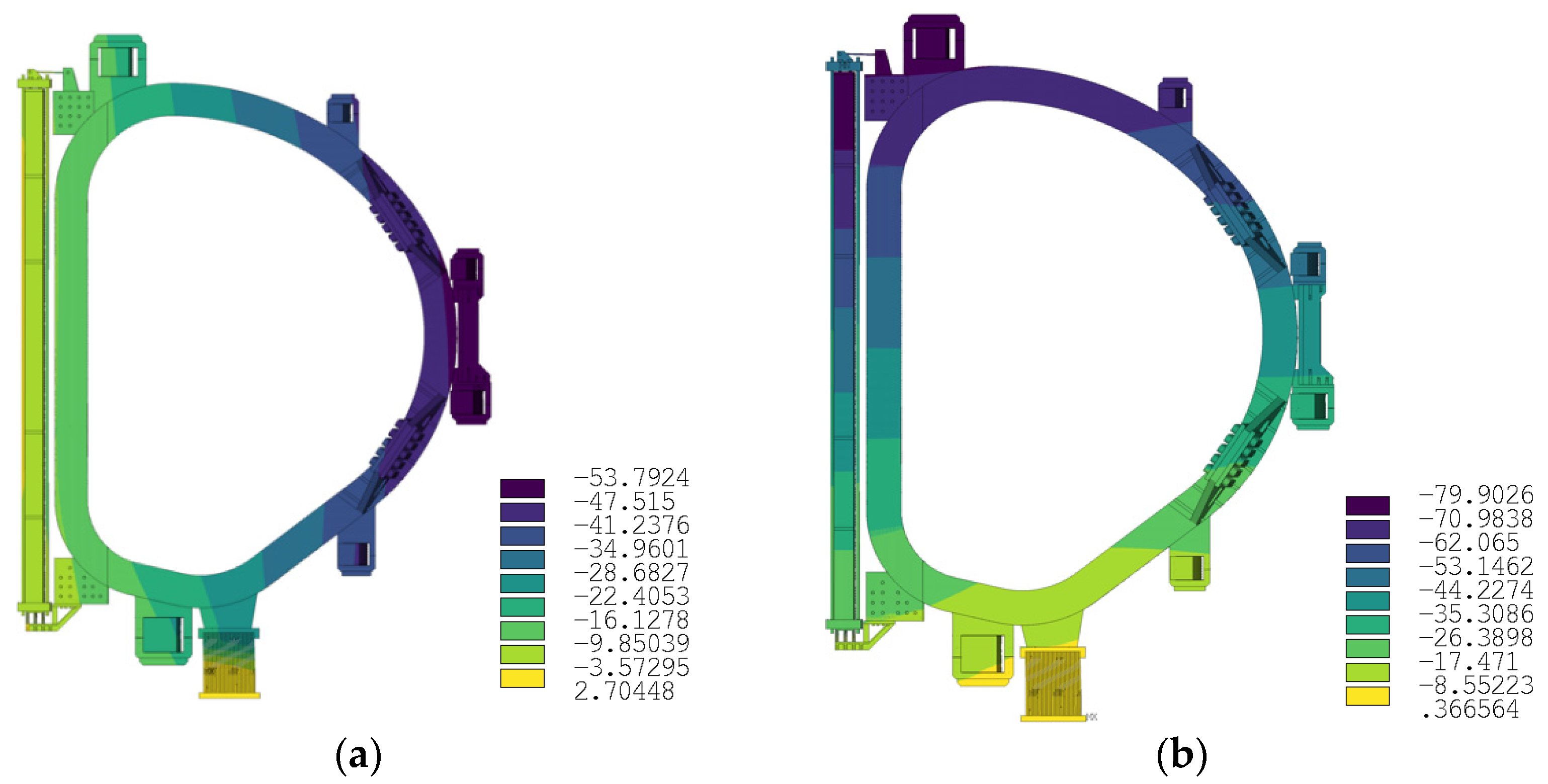
The results of the static analyses in terms of displacement components are reported in
Figure 11 at the end of the cooldown, in
Figure 12 at the TF energization phase and at the end of flattop.
The distributions of the Tresca stress at the end of the cooldown, at the end of the energization phase and at the end of flattop are shown in
Figure 13. As expected, the stress field is low at the end of the cooldown; it is significantly higher at the TF energization and reaches its maximum at the end of flattop due to the presence of the OOP forces. The stress concentrations are located on the case of the TF at the plasma side, where the winding pack detaches almost completely from the case lid (
Figure 14).
6. Fatigue Life Assessment—(S-N) Approach
For the fatigue assessment of the toroidal field coils and support structures (IIS, OIS and GS), the procedure adopted is based on the prescriptions of the ITER design criteria [
21,
22,
23,
24]. Considering the complete set of static analyses performed previously, it is possible to identify two time points corresponding to the minimum and maximum of the function describing the Tresca equivalent stress over time. Only the time interval involving cyclic loads must be considered, i.e., from the TF energization to the end of flattop. The radial and the vertical forces remain constant over time, while the OOP actions work as a superimposed cyclic load. The minimum is recorded at the energization phase (
Figure 15), which is the early stage of the plasma scenario. The maximum is reached at the end of flattop (
Figure 16) where the combination of in-plane and out-of-plane loads produces the highest stress peaks. As mentioned, to obtain a conservative estimate of the fatigue damage on the structure, it is assumed to have 20,000 constant cycles.
The procedure for the extraction of the equivalent alternate fatigue stress is made of the following steps:
- (a)
The six components (σ
x, σ
y, σ
z, τ
xy, τ
yz, τ
xz) of the stress tensor for each finite element are stored in two matrices, collecting the extremes of the stress cycle (
Figure 15 and
Figure 16). To this aim, a proper local coordinate system is defined for the elements considered. The x and z components are oriented, respectively, radially and toroidally along the TF curvilinear abscissa, while the y component is tangent to the curvilinear abscissa.
- (b)
The stress range matrix (σRx, σRy, σRz, τRxy, τRyz, τRxz) is computed by subtracting the minimum stress matrix from the maximum stress one.
- (c)
The three principal stresses (σR1, σR2, σR3) of the range matrix and the three principal direction cosines ((l,m,m)1, (l,m,n)2, (l,m,n)3) are computed.
- (d)
The “equivalent alternating stress” (S
alt) is defined as half the largest principal stress range difference: S
alt = 0.5 max|(σ
R1 − σ
R2), (σ
R2 − σ
R3), (σ
R1 − σ
R3)| (
Figure 17).
- (e)
The mean stress matrix (σmx, σmy, σmz, τmxy, τmyz, τmxz) is calculated from the two stress matrixes calculated in point (a).
- (f)
The three principal mean stresses (σm1, σm2, σm3) and the three principal direction cosines ((l,m,m)I, (l,m,n)II, (l,m,n)III) are calculated.
- (g)
The “equivalent mean stress” (Smean) is equal to the sum of the two principal mean stress components having the same direction cosines as the two principal stress range components determining the Salt value.
- (h)
The equivalent mean stress is finally corrected by adding the residual stress related to the base material, conventionally equal to 50 MPa, or to the weld regions, conventionally equal to 250 MPa (
Figure 18).
The equivalent mean stresses so obtained must be compared with the (S-N) experimental curve available for the 316LN at cryogenic temperature (4.2 K). Fatigue experimental tests on material samples are usually run for “constant amplitude-fully reversing cycles”, i.e., the same stress magnitude is applied in tension and in compression (which corresponds to a load ratio R = σ
min/σ
max = −1). On the contrary, the values of the equivalent alternating stress (S
alt) and the equivalent mean stress (S
mean) computed above represent a generic load cycle where the ratio between the minimum and the maximum stress value is not −1. It is therefore necessary to define a relation to correct the equivalent stresses obtained. Following the ITER criteria, a good compromise is provided by the Goodman relation, which gives the most accurate result for cryogenic applications. The equivalent stress amplitude
Seq is thus obtained as
where
σu is the ultimate strength of the material.
For the (S-N) fatigue life assessment, the allowable values are specified in the ITER design criteria: either a safety factor of 2 on the equivalent stress amplitude
Seq, or a safety factor of 20 on the cycles to failure, must be applied to the best fit of the material fatigue data. For the AISI 316LN (S-N) curve [
14], a safety factor of 2 on the equivalent stress amplitude always gives a more conservative limitation, and it has been chosen in our fatigue assessment. The (S-N) relation (best fit of the experimental data) that we employed reads
For N = 20,000 cycles, the resulting allowable value is
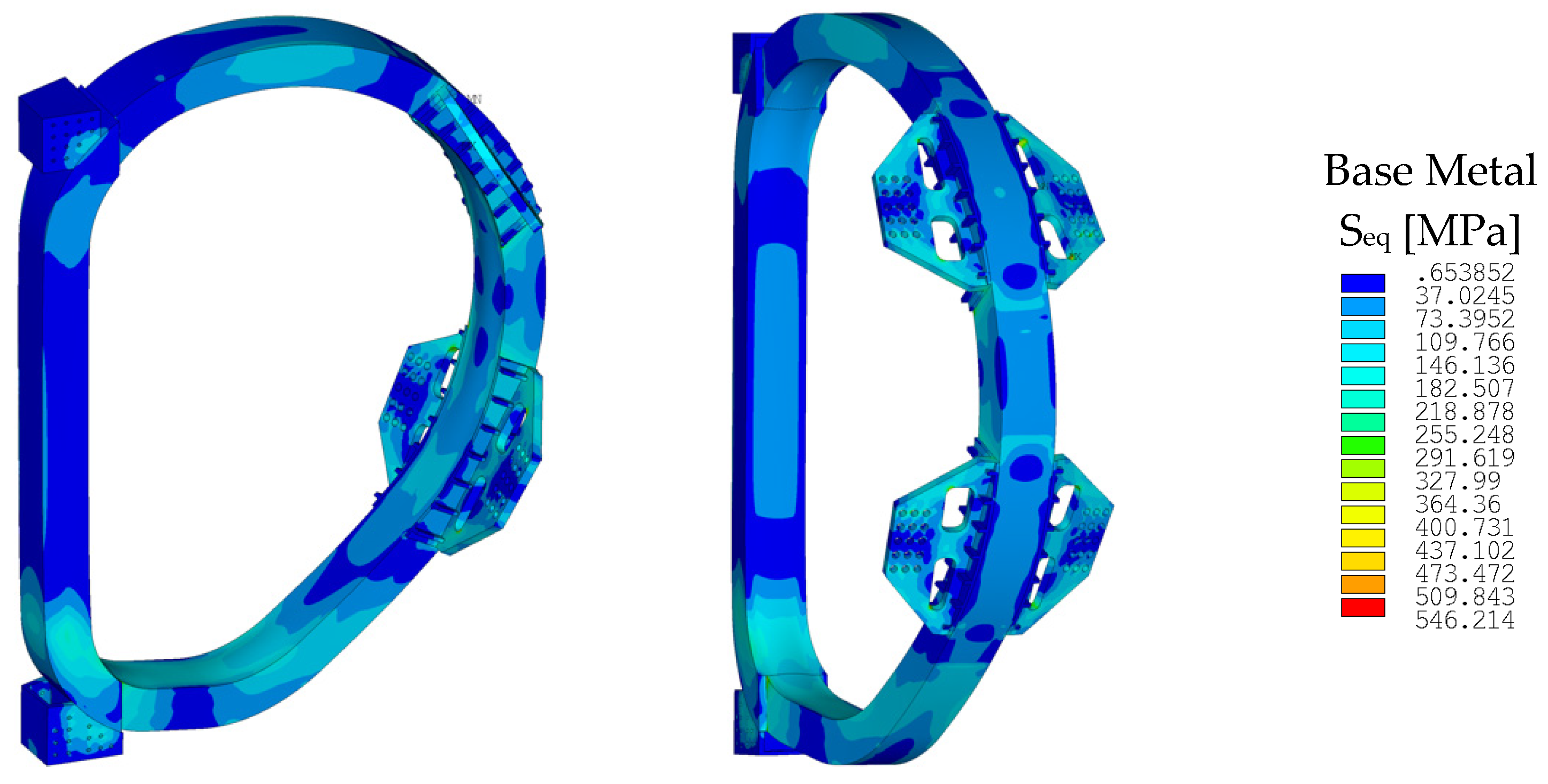
Seq = 462 MPa. As reported in
Figure 19 and
Figure 20, there are a few localized regions where the
Seq reaches the allowable value. In particular, in the analysis performed by considering the residual stress on the base metal (
Figure 19), the criterion is met for 99% of the elements. It means that a little change in the shape of the holes of the OIS shall be sufficient to solve the issue. Considering the residual stress on the weld (
Figure 20), the region where the
Seq values exceeds the limit is a little larger (in grey in
Figure 21b). However, this effect was expected since that zone is subject to stress concentration, being the connection between the TF coil and the upper OIS. In a following refinement of the design, that peak of stresses can be easily smoothed, e.g., by enlarging the connection plate.
7. Conclusions
A methodological approach is presented that explores the analyses performed on the TF coil system and its support structures. Two sequentially coupled parts are identified: the electromagnetic section (EMS) and the structural section (SS). Concerning the electromagnetic field, the full set of loading conditions included in the reference scenario is computed with a dedicated 3D finite element model. To this aim, EMS is further split into two sequentially coupled steps, the first one dealing with an electrostatic study, the second one with a magnetostatic analysis. The magnetic field, the magnetic flux and the Lorentz force exerted by the magnets are accurately investigated to have a better insight into the behavior of the machine. A consistent 3D structural model is then defined, comprising the three main magnetic systems and their support structures. To model the winding packs of the CS, PF and TF coils, a homogenization procedure is implemented, considering a proper representative volume element for each magnet and, for the TF winding pack, a different RVE for each cable of the twelve layers. The periodic boundary conditions applied are also detailed, together with the virtual tests performed to obtain the homogenized materials. Finally, the mechanical evaluation is completed by the fatigue assessment, via the (S-N) approach. To this aim, two time points (the TF energization and the end of flattop of the plasma scenario) are used to define the minimum and the maximum of the stress cycle. By considering the 20,000 plasma pulses scheduled for the machine, the equivalent Goodman stress is compared to the allowable limit for the AISI 316LN at the operating temperature. The final Seq field shows that there are only a few, very narrow areas where the limit is exceeded. The smoothing of those stress peaks can be easily obtained by an improvement of the design.


