Extending Contrastive Learning to Unsupervised Redundancy Identification

Abstract

Modern deep neural network (DNN)-based approaches have delivered great performance for computer vision tasks; however, they require a massive annotation cost due to their data-hungry nature. Hence, given a fixed budget and unlabeled examples, improving the quality of examples to be annotated is a clever step to obtain good generalization of DNN. One of key issues that could hurt the quality of examples is the presence of redundancy, in which the most examples exhibit similar visual context (e.g., same background). Redundant examples barely contribute to the performance but rather require additional annotation cost. Hence, prior to the annotation process, identifying redundancy is a key step to avoid unnecessary cost. In this work, we proved that the coreset score based on cosine similarity (cossim) is effective for identifying redundant examples. This is because the collective magnitude of the gradient over redundant examples exhibits a large value compared to the others. As a result, contrastive learning first attempts to reduce the loss of redundancy. Consequently, cossim for the redundancy set exhibited a high value (low coreset score). We first viewed the redundancy identification as the gradient magnitude. In this way, we effectively removed redundant examples from two datasets (KITTI, BDD10K), resulting in a better performance in terms of detection and semantic segmentation.

1. Introduction

Deep-learning-based approaches have been a key technique in various computer vision tasks, such as image classification [1], object detection [2], and image segmentation [3]. However, achieving an excellent performance usually entails two requirements: (i) a massive cost for annotating examples that usually require human labor and (ii) a good quality of annotated examples, that is, examples belonging to the same class that exhibit diverse appearances [4]. Therefore, to reduce the annotation cost while achieving a great performance, assessing the quality of unlabeled examples could be a key step. One of the issues that hinders the quality of the examples is the presence of redundancy. Clearly, many images with identical visual contents, such as nearly the same background and foreground, seldom contribute to the performance but could lead to a severe over-fitting. In general, a dataset with a large number of redundant examples may introduce bias and harm the generalization of the classifier regardless of the type of machine learning algorithm used. In addition, in terms of the annotation cost, these redundant examples require a higher annotation budget while exhibiting less fruitful features. In this regard, identifying redundant examples in an unlabeled dataset plays a crucial role in dataset refinement. As a result, one can obtain high-quality examples and reduce the annotation cost. It was discovered that redundant examples occupy a relatively large portion of well-known datasets [5]. However, few studies have focused on identifying redundancy, particularly for unlabeled data; thus, this topic remains an issue. The most related topic could be key frame detection, which aims to discover the frame that provides powerful features from a video. Yan et al. [6] recently achieved key frame detection in a self-supervised manner, that is, at zero annotation cost. They verified their method by applying a thorough experiment on an action recognition dataset. However, key frame detection is mostly concentrated on a video in which capturing the correlation between consecutive frames is a key technique; thus, it is an impossible approach for a dataset that consists of still images. Moreover, Ju et al. [7] achieved unsupervised coreset selection using a coreset score established by constrastive learning. Their goal was to identify the subset of unlabelled data, which exhibit high contribution to the performance. Hence, they built a coreset score that measures the level of contribution. Inspired by this work, we conjectured that a low coreset score might be able to capture redundancy. This is because redundant examples would obviously exhibit the low level of contribution, thereby being captured by the coreset score. Hence, we confirmed our conjecture via thorough experiment and theoretical analysis with a simple redundant set, where identical examples are present. Again, the aim of this study is to identify redundant examples from unlabeled datasets based on contrastive learning. Hence, prior to the annotation process, with our approach, redundancy scores are recommended that lead to an avoidance of unnecessary annotations. Our contributions are as follows:

• We extended the work [7] to identify redundant examples.
• We provided a theoretical explanation on the why coreset score established by contrastive learning is effective for capturing redundant examples.
• We built two different subsets from the entire unlabeled dataset; one with identified redundant examples removed, the other with examples randomly removed. Additionally, the quality of each subset was evaluated by training the existing DNN model for detection and segmentation tasks.

The rest of our paper is structured as follows. Section 2 summarizes recent literature on a topic of identifying redundancy and key-frame detection. Section 3 describes theoretical analysis to explain why the coreset score based on contrastive learning can measure the level of redundancy. Section 5 shows the experimental results in object detection and semantic segmentation tasks. Section 6 and Section 7 provide our conclusion and the limitation and future direction, respectively.

2. Related Work

2.1. Identifying Redundancy

Birodkar et al. [5] recently provided concrete proof that there exists significant redundancy in a popular dataset, such as CIFAR10, CIFAR100 [8], and ImageNet [4]. Hence, removing the identified redundant examples from the training set did not lead to a performance degradation. In addition, they claimed that these redundancies account for more than 10% of the training set. They achieved identified redundancy through supervised learning. Namely, they first obtained a semantic space that was established from ResNet [9] based on fully annotated examples. They then grouped examples in the space using the clustering method [10] and assumed that the resulting cluster represents each redundancy group. By doing so, except for representative examples that are closest to the center of each group, they identified the remaining examples as redundancy. However, note that their method is solely applicable to supervised learning, which requires fully annotated examples; hence, it does not reduce the annotation cost. In contrast, our study is mainly focused on identifying redundancy in the absence of an annotation, thus avoiding unnecessary annotations. In addition, there have been a few attempts to assess the priorities of examples and identify redundancy. Vodrahalli et al. [11] relied on the magnitude of the gradient of examples for importance sampling; that is, they regarded examples with the highest gradient as the most important subset of the training set. Carlini et al. [12] viewed the redundancy problem as a prototypical example, which claims to be in agreement with human intuition. However, these methods also demand fully annotated examples, which is the same as that in [5].

2.2. Key Frame Detection

The aim of our study agrees partly with the subject of key-frame detection, which aims to identify the most important frame and plays a key role in a given task. The topic of key-frame detection mostly deals with video; however, our study handles still images. Because the direct comparison between key frame detection and our approach was not fair, we introduces related research in this section. In one recently reported study, Yan et al. [6] provided a new method that required no annotation. Their proposed approach had a self-supervised learning framework that could identify the key frames in a video. The authors verified that their method was effective at detecting key frames for action recognition. In addition, numerous deep-learning-based approaches for key-frame detection ([13,14,15,16,17,18,19,20]) were proposed. They commonly considered the knowledge between consecutive frames to capture the correlation in a video, which is contrary to our approach.

3. Methods

We concentrated on the magnitude of the gradient of contrastive loss. As our underlying assumption, in which a low coreset score might be able to capture redundancy, the collective magnitude of the gradient for redundant examples may be relatively larger compared to that of non-redundant examples. This assumption was derived from a gradient calculation using simple examples, in which the same examples (extreme case of redundancy) were present in the dataset. We captured the gradient for each example through the cosine similarity (cossim), which can be readily obtained from contrastive learning. Furthermore, using the coreset score described in the literature [7], which is established based on cossim, we easily achieved a redundant identification by finding examples with the lowest coreset score. In this section, we provide a detailed theoretical perspective on why cossim exhibits high value for redundant examples, thereby resulting in a low coreset score.

Cossim for Redundant Examples

Consider a contrastive loss for SimCLR [21], which is described through the following equation:

$$l(z_i,z_j)=-log\frac{exp(sim(z_i,z_j)/\tau )}{{\sum }_{k=1}^{2N}{𝟙}_{\left[k\ne i\right]}exp(sim(z_i,z_k)/\tau )},$$

(1)

where $sim(u,v)=u^{T}v/\parallel u\parallel \parallel v\parallel$ denotes cossim, that is, the dot product between two vectors with $l_2$ normalization, and ${𝟙}_{\left[k\ne i\right]}\in \{0,1\}$ is the indicator function that yields a value of 1 if and only if $k\ne i$, and zero otherwise. In addition, $\tau$ is a temperature parameter and N is the number of positive examples. Hereafter, we used different notations for a clear understanding and provided a theoretical analysis of a contrastive loss on redundant examples.

Assume that we are given a neural network $F(·)=g(f(·))$ and a set of examples X. Here, $g(·)$ and $f(·)$ are the projection and feature extraction functions (refer to [21] for more detailed definitions of $g(·)$ and $f(·)$), respectively, and X is defined as follows:

$$\begin{array}{c}X=X_r\cup X_{nr},X_r\cap X_{nr}=\varnothing ,\\ X_r=\left\{x|x=x^{\prime },x\in X_r,x^{\prime }\in X_r\right\},\left|X_r\right|=M\\ X_{nr}=\left\{x|x\ne x^{\prime },x\in X_{nr},x^{\prime }\in X_{nr}\backslash \{x\}\right\},\left|X_{nr}\right|=N\end{array}$$

In other words, $X_r$ denotes a set of M identical examples (a set of redundant examples), i.e., an extreme case of redundancy, and $X_{nr}$ denotes a set of N different examples in which no redundant examples are present (a set of non-redundant examples). We draw two separate data augmentation functions from the same family of augmentations, $t\sim T$ and $t^{\prime }\sim T$, and sequentially apply the drawn augmentation function and $F(·)$ to each example such that $F(t(x))$ and $F(t^{\prime }(x))$. We obtain the following sets:

$$\begin{array}{c}{Z}_r=\left\{z|z=F(t(x)),x\in X_r\right\},\\ Z_r^{\prime }=\left\{z|z=F(t^{\prime }(x)),x\in X_r\right\},\\ Z_{nr}=\left\{z|z=F(t(x)),x\in X_{nr}\right\},\\ Z_{nr}^{\prime }=\left\{z|z=F(t^{\prime }(x)),x\in X_{nr}\right\}\\ {\mathbb{Z}}_r=\{(z,z^{\prime }):z=F(t(x)),z^{\prime }=F(t^{\prime }(x)),x\in X_r\}\\ {\mathbb{Z}}_{nr}=\{(z,z^{\prime }):z=F(t(x)),z^{\prime }=F(t^{\prime }(x)),x\in X_{nr}\}\end{array}$$

Using these notations, we rewrite Equation (1) (for brevity, we assume $\tau =1$) for z and $z^{\prime }$, i.e., $z=F(t(x))$, $z^{\prime }=F(t^{\prime }(x))$, and $x\in X_r$ as follows.

$$l(z,z^{\prime })=-log\frac{exp(sim(z,z^{\prime }))}{{\sum }_{\widehat{z}\in Z_r\backslash \{z\}}exp(sim(z,\widehat{z}))+{\sum }_{\widehat{z}\in Z_r^{\prime }}exp(sim(z,\widehat{z}))+{\sum }_{\widehat{z}\in Z_{nr}}exp(sim(z,\widehat{z}))+{\sum }_{\widehat{z}\in Z_{nr}^{\prime }}exp(sim(z,\widehat{z}))}$$

(2)

Similarly, for z and $z^{\prime }$, i.e., $z=F(t(x))$, $z^{\prime }=F(t^{\prime }(x))$, and $x\in X_{nr}$,

$$l(z,z^{\prime })=-log\frac{exp(sim(z,z^{\prime }))}{{\sum }_{\widehat{z}\in Z_r}exp(sim(z,\widehat{z}))+{\sum }_{\widehat{z}\in Z_r^{\prime }}exp(sim(z,\widehat{z}))+{\sum }_{\widehat{z}\in Z_{nr}\backslash \{z\}}exp(sim(z,\widehat{z}))+{\sum }_{\widehat{z}\in Z_{nr}^{\prime }}exp(sim(z,\widehat{z}))}$$

(3)

If we write the total loss for X, we can obtain the following equations:

$$\begin{array}{cc}\hfill L& =\frac{1}{N+M}\left(L^r+L^{nr}\right)\hfill \\ \hfill L^r& =\sum _{(z,z^{\prime })\in {\mathbb{Z}}_r}l(z,z^{\prime })+l(z^{\prime },z)\hfill \\ \hfill L^{nr}& =\sum _{(z,z^{\prime })\in {\mathbb{Z}}_{nr}}l(z,z^{\prime })+l(z^{\prime },z)\hfill \\ \hfill \end{array}$$

(4)

Note that the total loss is computed by a summation of pair losses ($l(z,z^{\prime })+l(z^{\prime },z)$), as described in [21]. In addition, if we calculate the gradient of the total loss, we can obtain

$$\begin{array}{c}\nabla L=\frac{1}{N+M}\left(\nabla L^r+\nabla L^{nr}\right)\\ \nabla L^r=\sum _{(z,z^{\prime })\in {\mathbb{Z}}_r}\nabla l(z,z^{\prime })+\nabla l(z^{\prime },z)\\ \nabla L^{nr}=\sum _{(z,z^{\prime })\in {\mathbb{Z}}_{nr}}\nabla l(z,z^{\prime })+\nabla l(z^{\prime },z)\end{array}$$

Recall that $X_r=\left\{x|x=x^{\prime },x\in X_r,x^{\prime }\in X_r\right\}$, which obviously results in $(z,z^{\prime })=(\widehat{z},{\widehat{z}}^{\prime })$, $(z,z^{\prime })\in {\mathbb{Z}}_r$, and $(\widehat{z},{\widehat{z}}^{\prime })\in {\mathbb{Z}}_r$. Considering Equation (3) again, the following can be obtained:

$$\nabla L^r=M\nabla l(z,z^{\prime })+M\nabla l(z,z^{\prime }),(z,z^{\prime })\in {\mathbb{Z}}_r.$$

(5)

As can be seen in Equation (5), a gradient of total loss for redundant examples is M-fold of a gradient of a single loss. In other words, the resulting gradient for redundant examples is multiplication of M and an identical gradient. This implies that SimCLR may update its parameters toward the direction of $\nabla L^{nr}$ in loss surface. However, a gradient of total loss for non-redundant examples ($\nabla L^r$) is a summation of individual gradient, which is not identical. Hence, we conclude that SimCLR is likely to reduce the total loss in the direction of the gradient for redundant examples. This will also result in the highest cossim for redundant examples. In contrast, the collective gradient of loss for non-redundant examples points in different directions, exhibiting a lower cossim compared to that of redundant examples. Consequently, we speculated that we were able to identify redundant examples using the cossim value. Therefore, we utilized the coreset scores (see Algorithm 1), as in the work [7], and proved that our assumption was correct based on thorough experiments.

Algorithm 1 building coreset score (Ju et al. [7])

input: unlabelled dataset S initialize metric $score\left[k\right]=0$, $k\in \{1,\dots ,sizeof(S)\}$, while SimCLR learning is not finished do  for all $k\in \{1,\dots ,sizeof(S)\}$ do    $score\left[k\right]=score\left[k\right]-cossim(z(k),z^{\prime }(k))$   # $z(k),z^{\prime }(k)$ are a latent positive pair of the k-th example $X=$ argsort ($score$, ascending order) return X

4. Datasets

4.1. KITTI 2D Object Detection Dataset

The KITTI dataset was established to evaluate the 2D object detection performance. It consists of 7481 training images and 7518 test images [22]. Each image has a resolution of approximately 1240 × 370 pixels. The names of the annotated classes and the numbers of their corresponding objects in the training set were car (40,037), van (2914), truck (1094), pedestrian (4487), person sitting (222), cyclist (1627), tram (511), and miscellaneous (973), totalling 51,865 objects.

4.1.1. Data Preparation

After observing each example in the training set, we noticed that there were hundreds of examples that exhibited similar visual contents (see Figure 1). These examples seemed to be images taken while the camera was still in the same location. The only difference between their visual content was that of a moving pedestrian. In this study, we regarded these examples as redundancies (441 examples). Because the test dataset was not accessible, we randomly divided the remaining training set (7040 examples) that had no redundant examples into a clean dataset (5000 examples) and a test set (2040 examples).

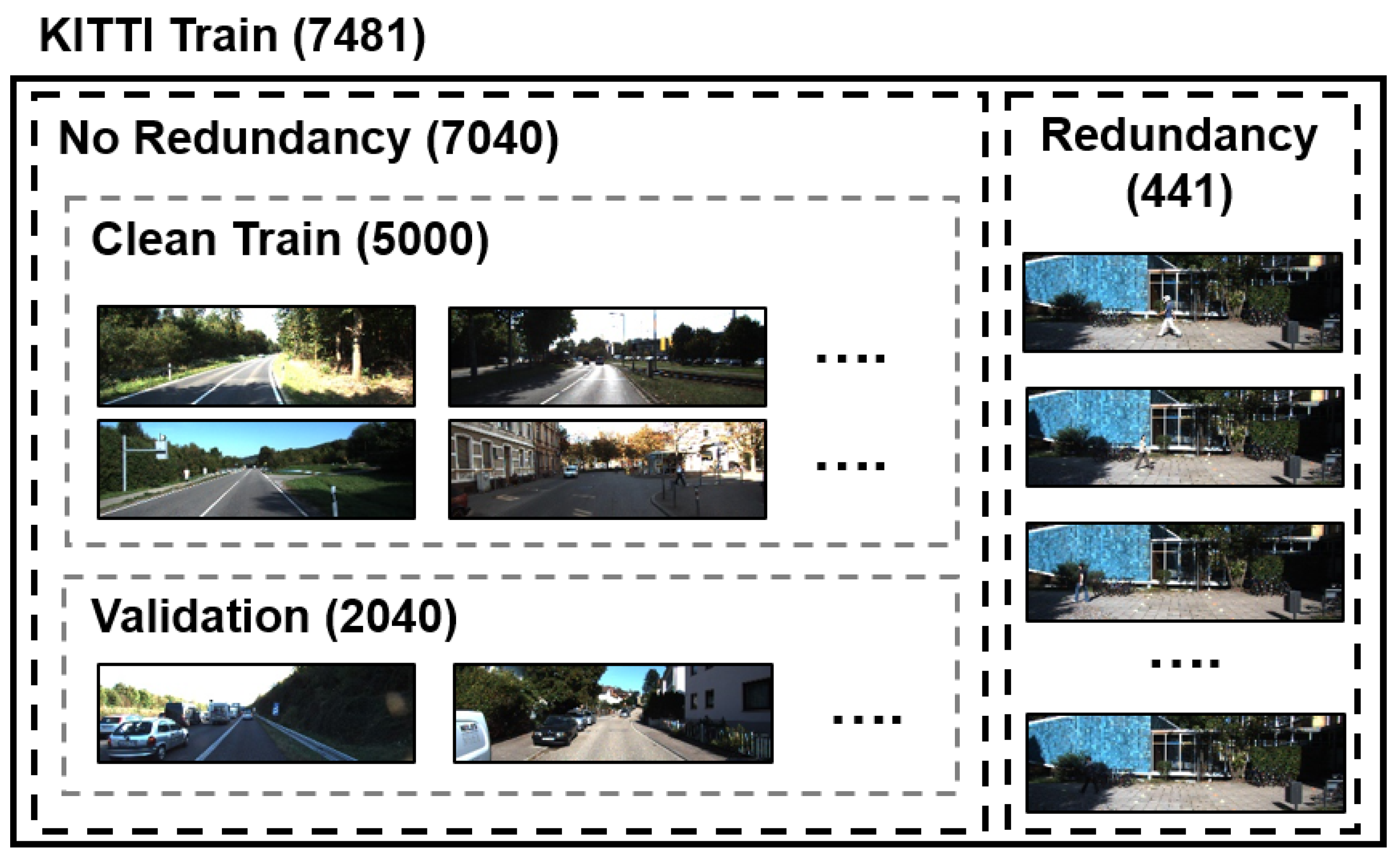
Figure 1. Our KITTI dataset preparation. The original KITTI dataset only provided 7481 examples of the training set. There were 441 examples that appeared to be nearly identical (see the redundancy). We split these redundancies from the original training set and randomly divided the remaining training set into a clean training set (5000) and a test set (2040). Consequently, we prepared the original training set to obtain a clean training set, redundancy set, and test set.

4.1.2. Data Refinement for Object Detection

We first augmented redundancy examples with two augmentation methods, that is, brightness and darkness. Figure 2 shows the results of such augmentations. In this way, we obtained 1323 (441 × 3) redundant examples. To summarize our resulting dataset, we obtained 6323 training examples (clean training examples + augmented redundant examples) and 2040 test examples for the object detection experiment.

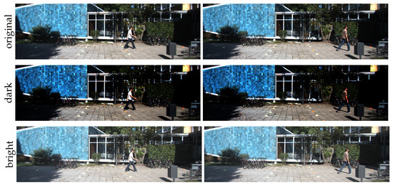
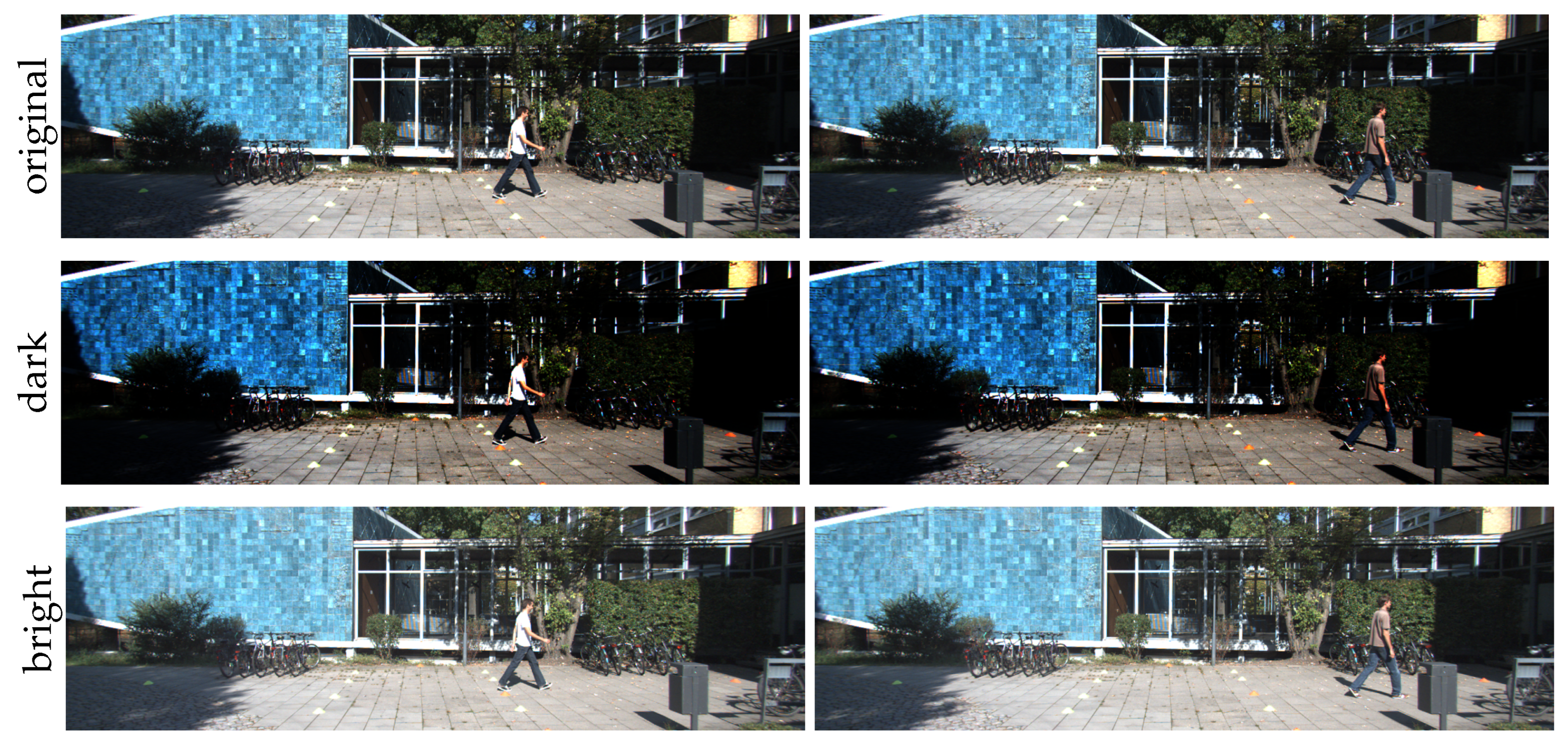
Figure 2. Augmentation results for redundant examples of KITTI. Original examples (top row), darkness (middle row), and brightness (bottom row) augmentation results for the original examples.

4.2. BDD10K

The BDD10K dataset [23] was constructed to evaluate the performance of semantic segmentation, instance segmentation, and panoptic segmentation and consisted of a training set (7000 examples), validation set (1000 examples), and test set (2000 examples). For semantic segmentation, there were 19 classes in total: road, sidewalk, building, wall, fence, pole, light, sign, vegetation, terrain, sky, person, rider, car, truck, bus, train, motorcycle, and bicycle. Each example had a resolution of 1280 × 720. Examples taken during the daytime or at night were mixed in the training and validation sets. In this study, we focused on semantic segmentation tasks and used a validation set as the test set because it is inaccessible to the annotations of the test set.

4.2.1. Data Preparation

Because our study does not focus on the variation in lighting conditions, we first removed 381 examples and 54 examples taken at night from the training and test sets, respectively, as shown in Figure 3. In addition, we defined redundant examples as those where the same visual contents continuously appeared in multiple frames and considered the remaining examples (6429) of the training set as the clean training set. Following this process, we obtained 6619 examples (clean train set + redundant examples) of our training set and 946 examples of the test set.

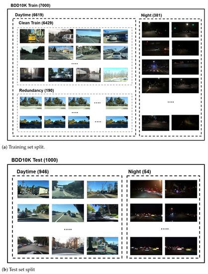
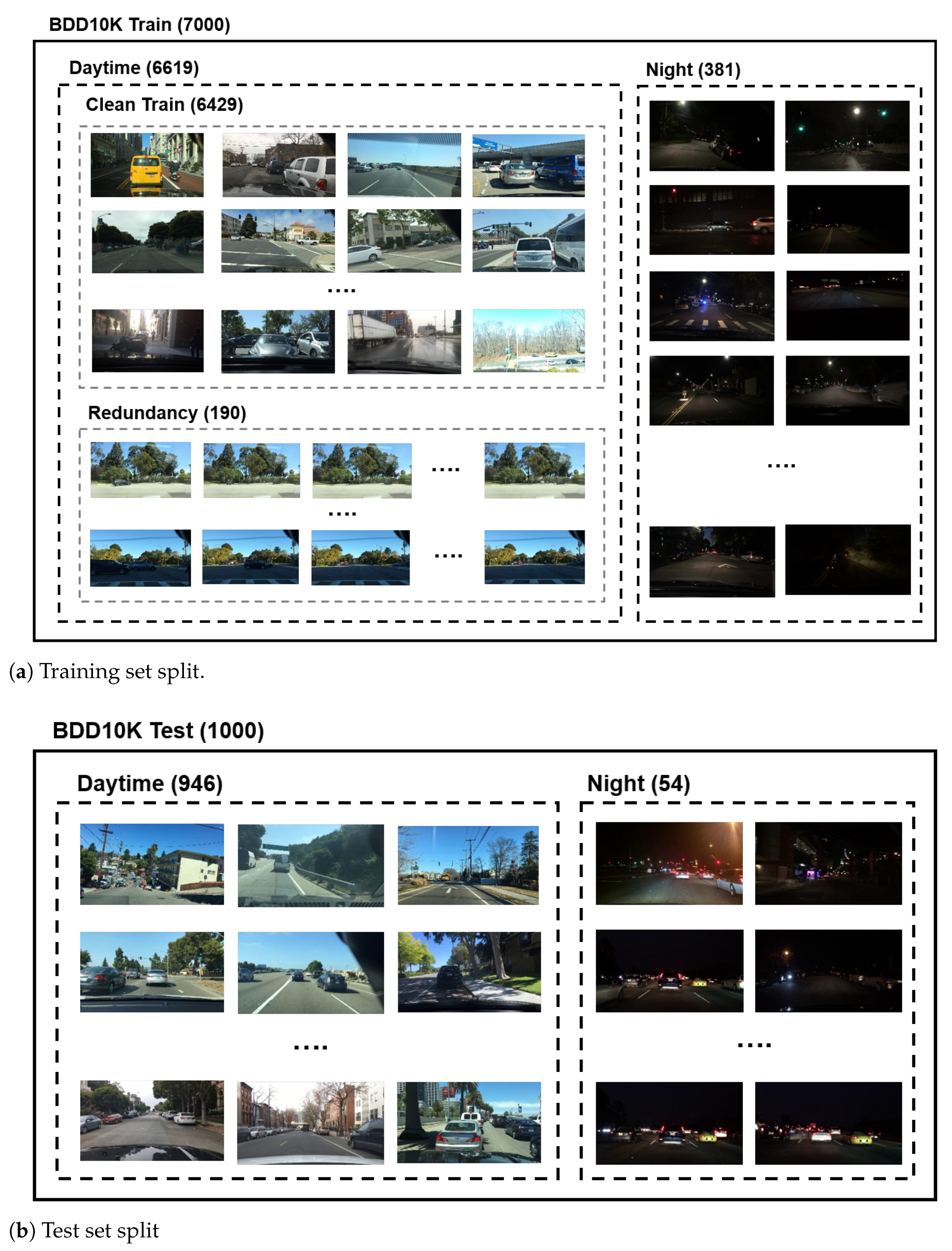
Figure 3. Our BDD10K dataset preparation. (a) The original BDD10K dataset provided 7000 examples of the training set. We first ignored 381 examples taken at night and did not use these examples for our experiment. We defined redundant examples as those that exhibited similar visual contents in multiple frames (at least four frames). In this regard, we identified 190 redundant examples from the original training set (see redundancy). We split these redundancies from the original training set and regarded the remaining examples as a clean training set. Consequently, we prepared the original training set to obtain a clean training set and a redundancy set. (b) Similar to the training set, we removed 54 examples taken at night from the original BDD 10 K test set. Thus, we obtained 946 examples for testing.

4.2.2. Data Refinement for Semantic Segmentation

For dataset refinement (see Figure 4), we applied augmentation on redundant examples using five methods: (i) darkness, (ii) brightness, (iii) flipping, (iv) a combination of flipping and darkness, and (v) a combination of flipping and brightness. In this way, we obtained 1140 (190 × 6) redundant examples. To summarize our resulting dataset, we obtained 7569 training examples (clean train examples + augmented redundant examples) and 946 test examples for the semantic segmentation experiment.

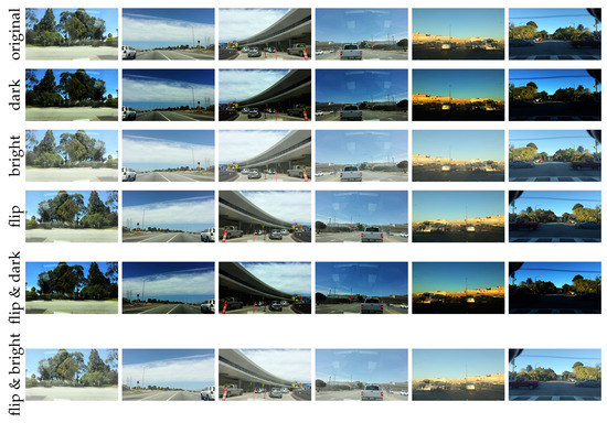
Figure 4. Augmentation results for redundant examples of BDD10K. Original examples (top row), and darkness (second row), brightness (third row), flipping (fourth row), flipping followed by darkness (fifth row), and flipping followed by brightness (bottom row) augmentation results for the original examples.

5. Experiments

5.1. Implementation Details

5.1.1. Contrastive Learning

We deployed ResNet18 [9] to achieve SimCLR across the dataset. Our coreset was constructed based on the code available on the website (https://github.com/Spijkervet/SimCLR (accessed on 1 December 2020)). Prior to starting SimCLR on two datasets (KITTI and BDD10K), to reduce the learning time, we first resized the examples of each dataset to 256 × 128 and 320 × 180 for KITTI and BDD10K, respectively. We set the hyper-parameters (batch size, number of epochs, and dimensions of the projection) to 200, 200, and 1024 for KITTI and 200, 1000, and 256 for BDD10K. We employed the LARS optimizer [24] across the datasets. For the augmentation techniques that were involved in SimCLR, we implemented randomly resized crops, random horizontal flipping, color jittering, and random grayscale.

5.1.2. Identifying Redundancy

Once SimCLR was completed on each dataset, we established the coreset scores based on cossim and sorted them (see Algorithm 1). Based on these sorted scores, we identified redundant examples given the training set. In other words, if one chooses the bottom 10% of the coreset scores for the training set, the chosen examples will be redundant.

5.1.3. Object Detection

For object detection on KITTI, we used YOLO-v5s (https://github.com/ultralytics/yolov5 (accessed on 1 October 2021)), which is an improved version of vanilla YOLO [25]. Once the building coreset score on the KITTI dataset was completed, we chose 1323 examples with the bottom coreset scores as redundant examples. Hence, we used the remaining examples (5000) to train YoLO-v5s. For comparison with the random selection method, we randomly selected 5000 out of 6323 examples (i.e., our refined training set). In this way, we prepared five different training subsets using different seeds to initialize the weights of the selection model (ResNet18). Thus, we proved that the object detection performance increased with our subset (which includes less redundancy) compared with the random subset (which includes more redundancy) with five runs. We set the batch size, learning rate scheduling, and number of epochs to 32, polynomial, and 300, respectively.

5.1.4. Semantic Segmentation

For semantic segmentation on BDD10K, we used DeepLab [26], which has been widely applied in image semantic segmentation. We employed ResNet50 [9] as the backbone model for the encoder part of DeepLab. Once the building coreset score on the BDD10K dataset was completed, we chose 1169 examples with the bottom coreset scores as redundant examples. Hence, we used the remaining examples (6400) to train DeepLab. For comparison with the random selection method, we randomly selected 6400 out of 7569 examples (i.e., our refined training set). In this way, we prepared five different training subsets using different seeds to initialize the weights of the selection model (ResNet18). Thus, we proved that the performance of the semantic segmentation increased with our subset (which includes less redundancy) compared with the random subset (which includes more redundancy) with five runs. We set the batch size, learning rate scheduling, and number of epochs to 24, linear, and 100, respectively.

5.2. Visual Inspection

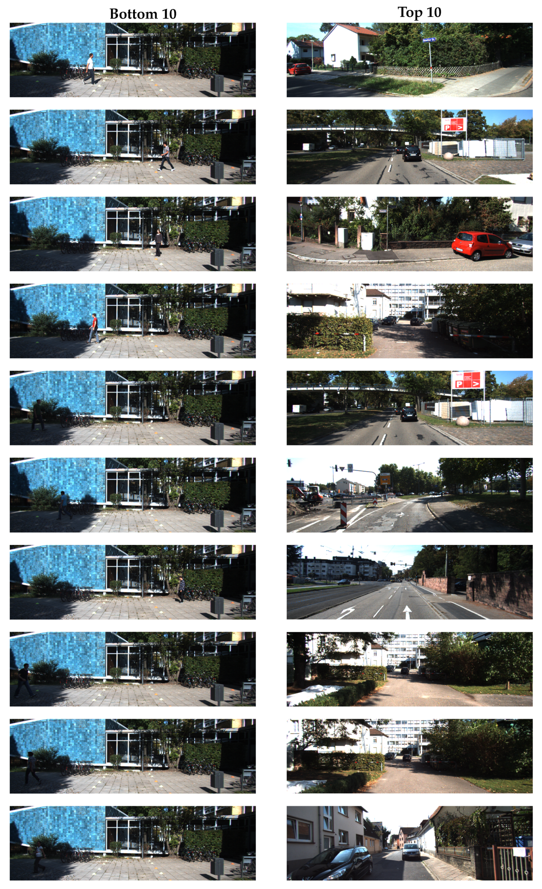
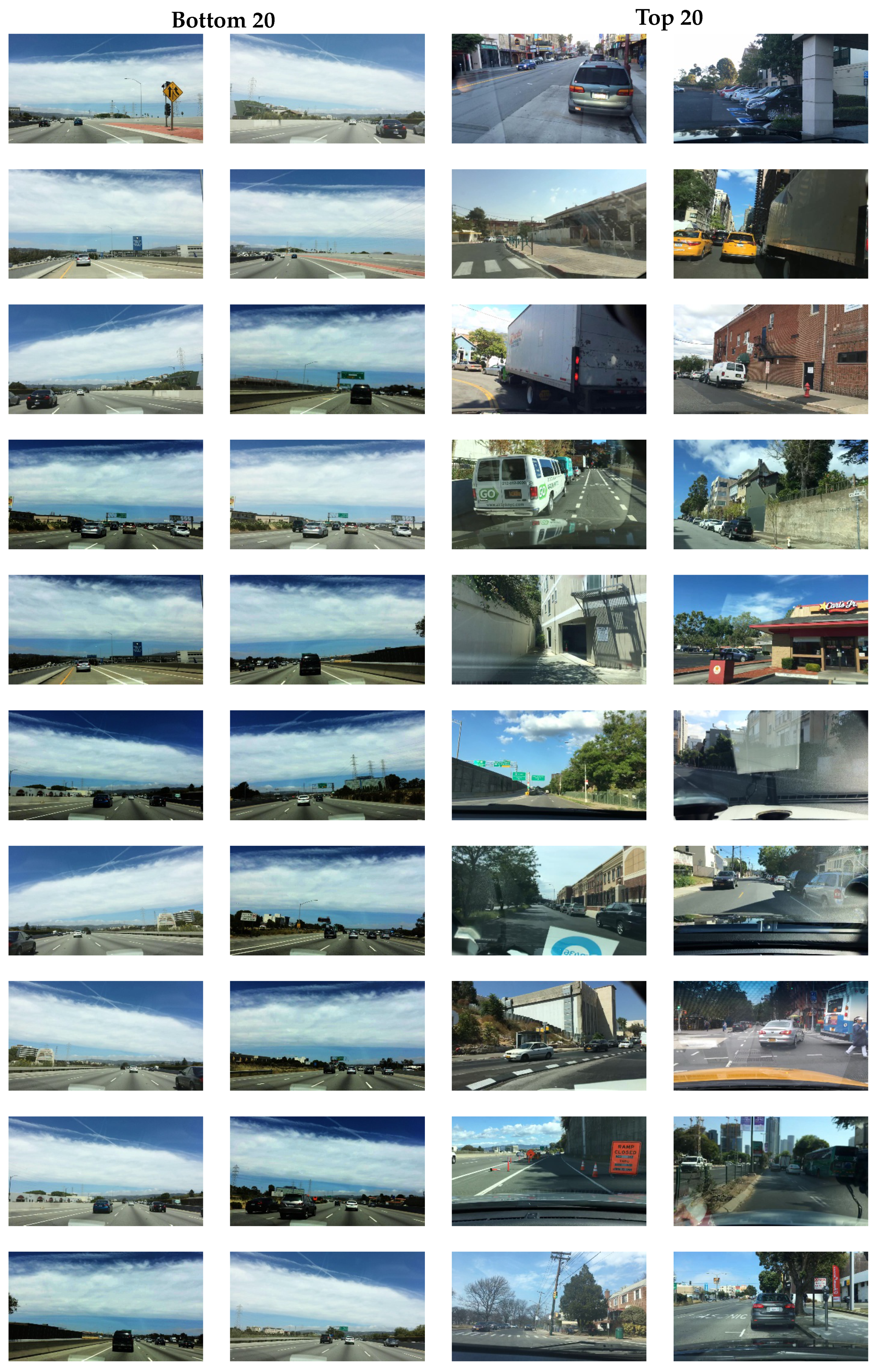
For a visual inspection on the KITTI dataset, we did not use our refined training set (clean train + augmented redundant examples); instead, we used our prepared training set (clean and redundant examples). In contrast, for visual inspection of BDD10K, we used our refined training set (clean and augmented redundant examples). To enable a thorough visual inspection, we identified the top and bottom 10 examples for KITTI and the top and bottom 20 examples for BDD10K using a single coreset score with SimCLR, as shown in Figure 5 and Figure 6. As shown in Figure 5, the top 10 examples exhibited various structures and patterns, i.e., they did not visually resemble one another and instead appeared dissimilar. In contrast, the bottom 10 examples primarily comprised nearly the same structures and backgrounds. The difference between them was the pedestrian, i.e., each image had a different person. Similarly, as shown in Figure 6, the top 20 examples exhibited various structures and patterns. In contrast, the bottom 20 examples primarily comprised nearly the same sky and road environments. The obvious difference between them was the type of car, i.e., each image had a different car. Hence, we conclude that our identification of redundant examples captures the redundancy fairly well.

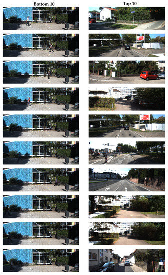
Figure 5. Visual inspection for KITTI. In total, 10 examples with a bottom coreset score (left column) showed a similar appearance. A total of 10 examples with a top coreset score (right column) were dissimilar in appearance to each other.

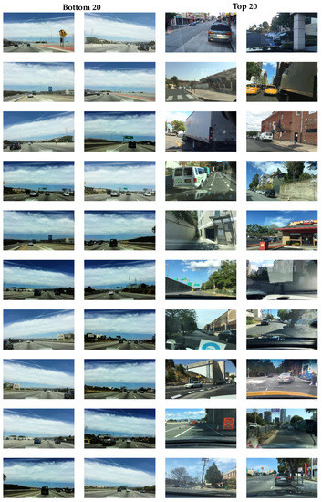
Figure 6. Visual inspection for BDD10K. In total, 20 examples with a bottom coreset score (left column) showed a similar appearance. A total of 20 examples with a top coreset score (right column) were dissimilar in appearance to each other.

5.3. Object Detection Task

Recall that our selection method removed 1323 examples of the identified redundancy from our refined training set (6323 examples) and we used the remaining subset (5000) to train YOLO-v5s. In contrast, the random selection method simply chose 5000 examples out of our refined training set. In this way, there were approximately 701 and 12 examples of true redundancy in the randomly selected subset and our subset, respectively. As listed in Table 1, we displayed the object detection performance with the mAP metric. We achieved an overall performance of 0.9326 in terms of mAP@0.5. Except for the misc class, the pedestrian class exhibited the largest improvement over the other classes. Notably, considering that our identified redundant examples were mostly composed of the same background and pedestrian, we conjectured that the improvement was due to a reduction in the over-fitting. In other words, because a randomly selected subset included more (nearly 60-fold) redundant examples compared to our subset, as a result, YOLO-v5s might suffer from an overfitting.

Table 1. Object detection performance on KITTI. The average ± std value was obtained from five runs. The number of instances represents the number of bounding boxes for each class in the test set. In addition, () denotes our improvement over random selection.

Selection		Instance	Performance Metric
Method	Class	Count	mAP@0.5	mAP@0.5:0.95
Our Selection	all	11,493	0.9326 ± 0.0032 (+0.0060)	0.7214 ± 0.0047 (+0.0176)
	car	8323	0.9810 ± 0.0000 (+0.0028)	0.8592 ± 0.0011 (+0.0116)
	van	805	0.9714 ± 0.0024 (+0.0038)	0.8336 ± 0.0030 (+0.0154)
	truck	313	0.9828 ± 0.0031 (+0.0032)	0.8582 ± 0.0070 (+0.0136)
	pedestrian	1110	0.8708 ± 0.0069 (+0.0136)	0.4970 ± 0.0041 (+0.0158)
	person sitting	73	0.7764 ± 0.0228 (−0.0132)	0.4584 ± 0.0260 (+0.0042)
	cyclist	439	0.9402 ± 0.0043 (+0.0112)	0.7034 ± 0.0050 (+0.0246)
	tram	157	0.9674 ± 0.0078 (+0.0106)	0.7628 ± 0.0106 (+0.0226)
	misc	273	0.9712 ± 0.0036 (+0.0172)	0.7712 ± 0.0024 (+0.0332)
Random Selection	all	11,493	0.9266 ± 0.0043	0.7038 ± 0.0024
	car	8323	0.9782 ± 0.0011	0.8476 ± 0.0023
	van	805	0.9676 ± 0.0024	0.8182 ± 0.0011
	truck	313	0.9796 ± 0.0029	0.8446 ± 0.0047
	pedestrian	1110	0.8572 ± 0.0068	0.4812 ± 0.0040
	person sitting	73	0.7896 ± 0.0377	0.4812 ± 0.0135
	cyclist	439	0.9290 ± 0.0033	0.6788 ± 0.0082
	tram	157	0.9568 ± 0.0040	0.7402 ± 0.0073
	misc	273	0.9540 ± 0.0080	0.7380 ± 0.0098

5.4. Semantic Segmentation Task

Recall that our selection method removed 1219 examples of the identified redundancy from our refined training set and we used the remaining subset (6400) to train DeepLab. In contrast, the random selection method simply chose 6400 examples out of our refined training set. In this way, there were approximately 641 and 87 examples of true redundancy in the randomly selected subset and our subset, respectively. As listed in Table 2, we displayed a semantic segmentation performance in terms of the IoU for each class and the overall performance in terms of the mIoU. We achieved a 0.5614 mIoU and an improvement of +0.0381 compared with random selection. First, we consider both the number of pixels and the IoU performance. We counted the number of pixels in the test set in terms of percentage. It was obvious that there was a strong correlation between the number of pixels and the IoU performance. Namely, as the number of pixels increased, the IoU also exhibited a higher value for both our method and random selection. Hence, because the pixels belonging to the road class occupied the highest percentage of total pixels, the corresponding IoU showed the highest values. In contrast, the class with the least number of pixels, that is, the train class, achieved a performance of nearly zero. Apart from the wall, terrain, and rider classes, our selection methods outperformed the random methods. Particularly for the motorcycle class, we observed the highest improvement (+0.2831). We conjecture that the redundant training examples removed for random selection may include more motorcycles than that of our selection.

Table 2. Semantic segmentation performance on BDD10K dataset. The average ± std was obtained for the three runs. We measured the performance for each class using the IoU for all classes with the mIoU. In addition, we counted the pixels for each class in the test set in terms of percentage (second column). Notably, because pixels belonging to the training class exhibited a performance of nearly zero (0.01), both selection methods failed to capture the train.

	Pixel	Our	Random
Class	Count (%)	Selection	Selection
all	100	0.5614 ± 0.0017 (+0.0381)	0.5233 ± 0.0018
road	24.76	0.9367 ± 0.0002 (+0.0013)	0.9654 ± 0.0010
sidewalk	2.41	0.5963 ± 0.0014 (+0.0028)	0.5935 ± 0.0050
building	17.13	0.8384 ± 0.0003 (+0.0002)	0.8382 ± 0.0010
wall	0.40	0.2550 ± 0.0177 (−0.0217)	0.2767 ± 0.0339
fence	0.97	0.4955 ± 0.0007 (+0.0106)	0.4849 ± 0.0116
pole	1.18	0.4566 ± 0.0026 (+0.0098)	0.4468 ± 0.0060
light	0.16	0.5111 ± 0.0017 (+0.0096)	0.5015 ± 0.0026
sign	0.27	0.4700 ± 0.0067 (+0.0007)	0.4693 ± 0.0079
vegetation	18.21	0.8571 ± 0.0004 (+0.0009)	0.8562 ± 0.0003
terrain	1.07	0.4795 ± 0.0020 (−0.0024)	0.4819 ± 0.0049
sky	20.62	0.9588 ± 0.0005 (+0.0026)	0.9562 ± 0.0004
person	0.29	0.6557 ± 0.0047 (+0.0048)	0.6510 ± 0.0051
rider	24.75	0.0000 ± 0.0000 (−0.0024)	0.0024 ± 0.0042
car	10.54	0.8900 ± 0.0005 (+0.0006)	0.8895 ± 0.0007
truck	1.19	0.5169 ± 0.0069 (+0.0101)	0.5068 ± 0.0059
bus	0.73	0.7822 ± 0.0004 (+0.0062)	0.7760 ± 0.0029
train	0.01	0.0000 ± 0.0000 (+0.0000)	0.0000 ± 0.0000
motorcycle	0.03	0.4289 ± 0.0133 (+0.2831)	0.1458 ± 0.2525
bicycle	0.02	0.5390 ± 0.0297 (+0.1795)	0.3596 ± 0.1779

6. Conclusions

In this paper, we prove that the coreset score establised by contrastvie learning is effective for identifying redundant examples. Considering coreset selection task [7], the main assumption was that a low cossim represents coreset examples; however, for the redundant identification problem, we focused on cossim in a reverse manner. Namely, a high cossim has the power to represent a redundant example. This is because the collective magnitude of the gradient over redundant examples exhibits a large value compared to the others. As a result, contrastive learning first attempts to reduce the loss of redundancy. Consequently, cossim for the redundancy set exhibited a high value (low coreset score). We first viewed the redundancy identification as the gradient magnitude. In this way, we effectively removed redundant examples from the dataset, resulting in a better performance in terms of detection and semantic segmentation.

7. Discussion

As can be seen in the KITTI dataset, there could be a high probability of taking redundant examples in real world scenarios. Those examples carry similar visual context but exhibit a low level of contribution to performance. Given a fixed budget, avoiding redundant examples annotation is essential before the annotation process starts. Hence, our work can play the role of identifying redundant examples with the absence of annotations. However, there are limitations to our study, which can be directions for future research.

• Although we proved that cossim is appropriate for identifying a redundancy, the problem of defining a new metric better tailored to identifying redundancy should be addressed. The other future direction could be defining a new loss function, such that the DNN explicitly captures redundant examples. Our current work did not define the loss function but utilized a contrastive loss function.
• For simplicity, we depended on the heuristic method through a human visual inspection to define redundant examples. However, the precise definition of redundancy could help derive a clear objective function.

Finally, we hope that our study provides insight for future research on advanced methods for reducing redundant examples.

References

- Pak, M.; Kim, S. A review of deep learning in image recognition. In Proceedings of the 2017 4th International Conference on Computer Applications and Information Processing Technology (CAIPT), Kuta Bali, Indonesia, 8–10 August 2017; pp. 1–3. [Google Scholar]
- Masita, K.L.; Hasan, A.N.; Shongwe, T. Deep learning in object detection: A review. In Proceedings of the 2020 International Conference on Artificial Intelligence, Big Data, Computing and Data Communication Systems (icABCD), Durban, South Africa, 6–7 August 2020; pp. 1–11. [Google Scholar]
- Minaee, S.; Boykov, Y.Y.; Porikli, F.; Plaza, A.J.; Kehtarnavaz, N.; Terzopoulos, D. Image segmentation using deep learning: A survey. IEEE Trans. Pattern Anal. Mach. Intell. 2021. [Google Scholar] [CrossRef] [PubMed]
- Deng, J.; Dong, W.; Socher, R.; Li, L.J.; Li, K.; Fei-Fei, L. Imagenet: A large-scale hierarchical image database. In Proceedings of the 2009 IEEE Conference on Computer Vision and Pattern Recognition, Miami, FL, USA, 20–25 June 2009; pp. 248–255. [Google Scholar]
- Birodkar, V.; Mobahi, H.; Bengio, S. Semantic Redundancies in Image-Classification Datasets: The 10% You Don’t Need. arXiv 2019, arXiv:1901.11409. [Google Scholar]
- Yan, X.; Gilani, S.Z.; Feng, M.; Zhang, L.; Qin, H.; Mian, A. Self-supervised learning to detect key frames in videos. Sensors 2020, 20, 6941. [Google Scholar] [CrossRef] [PubMed]
- Ju, J.; Jung, H.; Oh, Y.; Kim, J. Extending Contrastive Learning to Unsupervised Coreset Selection. IEEE Access 2022, 10, 7704–7715. [Google Scholar] [CrossRef]
- Krizhevsky, A.; Hinton, G. Learning Multiple Layers of Features from Tiny Images. 2009. Available online: https://www.cs.toronto.edu/~kriz/cifar.html (accessed on 1 December 2020).
- He, K.; Zhang, X.; Ren, S.; Sun, J. Deep residual learning for image recognition. In Proceedings of the IEEE conference on computer vision and pattern recognition, Las Vegas, NV, USA, 27–30 June 2016; pp. 770–778. [Google Scholar]
- Defays, D. An efficient algorithm for a complete link method. Comput. J. 1977, 20, 364–366. [Google Scholar] [CrossRef] [Green Version]
- Vodrahalli, K.; Li, K.; Malik, J. Are all training examples created equal? an empirical study. arXiv 2018, arXiv:1811.12569. [Google Scholar]
- Carlini, N.; Erlingsson, U.; Papernot, N. Prototypical Examples in Deep Learning: Metrics, Characteristics, and Utility. 2018. Available online: https://openreview.net/forum?id=r1xyx3R9tQ (accessed on 1 December 2020).
- Li, X.; Zhao, B.; Lu, X. Key frame extraction in the summary space. IEEE Trans. Cybern. 2017, 48, 1923–1934. [Google Scholar] [CrossRef] [PubMed]
- Mahasseni, B.; Lam, M.; Todorovic, S. Unsupervised video summarization with adversarial lstm networks. In Proceedings of the IEEE conference on Computer Vision and Pattern Recognition, Honolulu, HI, USA, 21–26 July 2017; pp. 202–211. [Google Scholar]
- Huang, C.; Wang, H. A novel key-frames selection framework for comprehensive video summarization. IEEE Trans. Circuits Syst. Video Technol. 2019, 30, 577–589. [Google Scholar] [CrossRef]
- Sheng, L.; Xu, D.; Ouyang, W.; Wang, X. Unsupervised collaborative learning of keyframe detection and visual odometry towards monocular deep slam. In Proceedings of the IEEE/CVF International Conference on Computer Vision, Seoul, Korea, 27–28 October 2019; pp. 4302–4311. [Google Scholar]
- Wen, S.; Liu, W.; Yang, Y.; Huang, T.; Zeng, Z. Generating realistic videos from keyframes with concatenated GANs. IEEE Trans. Circuits Syst. Video Technol. 2018, 29, 2337–2348. [Google Scholar] [CrossRef]
- Kar, A.; Rai, N.; Sikka, K.; Sharma, G. Adascan: Adaptive scan pooling in deep convolutional neural networks for human action recognition in videos. In Proceedings of the IEEE Conference on Computer Vision and Pattern Recognition, Honolulu, HI, USA, 21–26 July 2017; pp. 3376–3385. [Google Scholar]
- Jian, M.; Zhang, S.; Wu, L.; Zhang, S.; Wang, X.; He, Y. Deep key frame extraction for sport training. Neurocomputing 2019, 328, 147–156. [Google Scholar] [CrossRef]
- Gharahbagh, A.A.; Hajihashemi, V.; Ferreira, M.C.; Machado, J.J.M.; Tavares, J.M.R.S. Best Frame Selection to Enhance Training Step Efficiency in Video-Based Human Action Recognition. Appl. Sci. 2022, 12, 1830. [Google Scholar] [CrossRef]
- Chen, T.; Kornblith, S.; Norouzi, M.; Hinton, G. A simple framework for contrastive learning of visual representations. In Proceedings of the International Conference on Machine Learning, Virtual Location, 12–18 July 2020; pp. 1597–1607. [Google Scholar]
- Geiger, A.; Lenz, P.; Urtasun, R. Are we ready for Autonomous Driving? The KITTI Vision Benchmark Suite. In Proceedings of the Conference on Computer Vision and Pattern Recognition (CVPR), Providence, Rhode Island, 16–21 June 2012; pp. 3354–3361. [Google Scholar]
- Yu, F.; Chen, H.; Wang, X.; Xian, W.; Chen, Y.; Liu, F.; Madhavan, V.; Darrell, T. Bdd100k: A diverse driving dataset for heterogeneous multitask learning. In Proceedings of the IEEE/CVF Conference on Computer Vision and Pattern Recognition, Seattle, WA, USA, 13–19 June 2020; pp. 2636–2645. [Google Scholar]
- You, Y.; Gitman, I.; Ginsburg, B. Large batch training of convolutional networks. arXiv 2017, arXiv:1708.03888. [Google Scholar]
- Redmon, J.; Divvala, S.; Girshick, R.; Farhadi, A. You only look once: Unified, real-time object detection. In Proceedings of the IEEE Conference on Computer Vision and Pattern Recognition, Honolulu, HI, USA, 21–26 July 2016; pp. 779–788. [Google Scholar]
- Chen, L.C.; Papandreou, G.; Kokkinos, I.; Murphy, K.; Yuille, A.L. Deeplab: Semantic image segmentation with deep convolutional nets, atrous convolution, and fully connected crfs. IEEE Trans. Pattern Anal. Mach. Intell. 2017, 40, 834–848. [Google Scholar] [CrossRef] [PubMed] [Green Version]
Publisher’s Note: MDPI stays neutral with regard to jurisdictional claims in published maps and institutional affiliations. |
© 2022 by the authors. Licensee MDPI, Basel, Switzerland. This article is an open access article distributed under the terms and conditions of the Creative Commons Attribution (CC BY) license (https://creativecommons.org/licenses/by/4.0/).