Abstract
Particulate volume scattering function (VSF), especially at angles larger than 170°, is of particular importance for interpreting ocean optical remote sensing signals and underwater imagery. In this study, a laboratory-based VSF instrument (VSFlab) adopting the periscopic optical system was developed to obtain VSF measurements from 1°–178.5°. In the VSFlab, a new prism design that simply combines a single prism and a neutral density filter was proposed to more efficiently reduce the stray light in the backward direction, while a detailed calibration procedure was given. A full validation based on standard beads of various sizes and a comparison with the results from LISST-VSF and POLVSM indicated that the VSFlab can provide reliable results from 1° to 178.5°. VSFlab measurements in the East China Sea (ECS) exhibited a moderate increase (not more than 5 times) in VSF from 170° to 178.5° rather than a sharp increase of more than one order of magnitude presented in other instrument results measured in other coastal regions. The estimates of the particulate backscattering coefficient using single angle scattering measurements near 120° or 140° and suitable χp were justified. Two types of the VSFs with different size distribution and shape parameters in the ECS can be distinguished based on the variability of χp after 155°. The measured VSF could provide a basis for the parameterization of VSF in the radiative transfer model and the variability of χp in the backward direction had the potential to be used to characterize the particles in the coastal region of the ECS.
1. Introduction
The volume scattering function (VSF), which describes the angular distribution of the scattered light resulting from an incident beam interacting with an infinitesimally small volume of water, is a fundamental inherent optical property (IOP) of the ocean [1,2,3,4]. It is generally defined as the radiant intensity I scattered from a volume element at scattering angle θ per unit of incident irradiance E and per unit of scattering volume V:
Based on Equation (1), the scattering coefficient, b, can be directly related to the VSF through Equation (2):
The VSF is often normalized by b to yield the phase function,
which provides information about the relative angular distribution of the scattering. The knowledge of the VSFs is of central importance for understanding the full radiative flux balance of the ocean [5,6,7,8]. The VSF in the backward direction is critical to interpreting ocean color remote sensing as the bidirectional distribution of the upwelling radiance has been shown to be largely governed by the shape of the VSF in the backward direction [9].
The VSF’s measurements can be traced back to the 1950s–1980s [10,11,12,13,14,15,16]. Measurement of the scattered light is made between 10° and 170° as the projector containing the light source rotates around the sample volume in Petzold’s instrument [13]. Such a design in which either a light source or another component (i.e., a single detector) rotates around the sample volume was commonly applied for wide-angle VSF detection and generally has advantages of high angular resolution and convenient calibration procedure [17,18,19,20,21,22,23]. Lotsberg et al. proposed a novel optical design that the photomultiplier (PMT) rotates around the scattering sample to measure the VSF from 3° to 171° with an angular resolution of 1° [18]. Similarly, Zugger et al. [19] and Svensen et al. [20] installed the rotatable detector in their instruments to measure the VSF from 1° to 170° (angular resolution of 1°) and full Muller matrix measurements from 16° to 160° (angular resolution of 2°), respectively. Measuring the signal at high backscattering angles (>170°) is hard for the above instruments. That is because the detector is performed in the same plane as the plane which contains the light source, the shadow of the light source masks the detector when this latter is positioned to the high backscattering angles. To distinguish between the plane of the light source from the plane of the detector, Lee and Lewis [21] proposed a periscopic optical system to change the propagation direction of scattered light and thus the detector and the light source are not in the same plane. For measurement at general angles, the periscopic prism rotates around the photodetector assembly axis that extends through the center of the scattering volume. For measurement at angles near 0°, the periscope prism was designed with a parallel shift such that the beam edge slides along the prism boundary and no direct light is received. MVSM utilized two strategies to measure VSF between 0.5° and 179°. The rotatable periscopic prism increases more instability of the optical path compared with the structure of the fixed prism and rotatable detector.
Recently, Chami et al. [23] proposed a new instrument called Polarized Volume Scattering Meter (POLVSM). Only one strategy based on the rotating-detector principle realized the VSF measurement between 1° and 179°. Two customized prisms called “P1” and “P2” were used to form a double periscopic optical system. The prism P1 is designed to guide the incident beam into the basin filled with water samples, while the role of the prism P2 is to guide the direct light outside the basin. Without P2, the specular reflection of the direct light onto the boundaries of the basin could induce a sharp increase in the VSF at a backward angle (i.e., typically from 150°). To avoid the direct light reflected back to the basin, an air gap was constructed inside the P2. However, during our practice, the manufacture of the P2 is not easy because it is easily broken when creating the air gap. Additionally, polishing the surface of the air gap is another challenge as limited space. The roughness of the air gap surface can cause undesirable diffuse stray light back to the basin and thus overestimation of VSFs in backward direction near 180°.
At present, measurements of total attenuation coefficient, absorption and scattering coefficient of suspended particles, and absorption coefficient of CDOM had been carried out in the East China Sea (ESC), but the VSF had not been measured and studied yet. The main reason was the lack of suitable instruments. The angle range and angle resolution of the rentable instrument are limited. The instrument developed by Li et al. [24] has only seven measurement angles, covering the angles from 20°–160°. Liao et al. [25] developed a laboratory prototype suitable for measuring the scattered light of submicron particles (0.1–0.8 μm), but the accuracy for larger beads (such as 11 μm) was limited and forward (near 0°) and backward VSF (near 180°) measurement accuracy were unclear. Wang et al. [26] manufactured the three-dimensional VSF instrument covering the angles from 18°–160°. The commercial instrument LISST-VSF could only reach 150° at backward direction [27].
The aim of the study is to establish a benchtop VSF instrument called VSFLab and study natural features of VSF from 1° to 178.5° in the coastal region of the ECS. The VSFlab instrument is established based on the principle of the double periscopic optical system and rotating detector. A simple design prism combing a single prism and a neutral density (ND) filter, which is easier to be fabricated with considerable efficiency in the stray light reduction, was designed and used. For confirming measurement accuracy, a detailed calibration procedure accounting for the rigorous validation works and comparison with LISST-VSF and POLVSM were carried out through the measurements in DUKE standard beads samples. The features of VSF in the ESC were analyzed by comparison with VSFs in other coastal regions. The χp factor derived from VSF was used to study the relationship between the shape of the particulate VSF in the backward direction and particle characteristics (i.e., diameter and so on).
2. Materials and Methods
2.1. Instrument Specification
The VSFlab instrument is established based on the principle of the double periscopic optical system and rotating detector, which is similar to that of Chami et al. [23]. In addition, the module of the attenuation coefficient (c) measurement is set up so that the samples’ attenuation coefficients and VSFs can be measured simultaneously. The overall schematic is illustrated in Figure 1a. The laser source’s wavelength is 532 nm (as an alternative, the 520 nm CW laser module of MatchBoxTM is available), and the divergence is about 0.06° at a half angle. The typical power is 60 mW. The laser source, together with a 1 mm pinhole, is fixed in an adjustor that allows one axial translation and two axial rotations. A beam splitter (R:T = 10:90) divides the laser into two beams. To monitor the fluctuation of the laser, we record the reflected beam with a photodetector, which also serves as the reference for c measurements. Through prism 1, the transmitted beam enters the sample inside the basin. Some of the transmitted beam is scattered at different angles, some is absorbed by the water, and some is reflected from the water onto the glass surface of the new prism and absorbed by the bottom of the basin whose absorptivity is 99.99% after the process of oxidative blackening. The remaining beam leaves the sample via the new prism and is then detected by another photodetector, whose minimum detectable power is about 2.4 × 10⁻¹⁴ , to determine the sample’s attenuation coefficient. The periscopic optical system, which contains a mirror, prism 1, and the new prism, separates the plane containing the scattered light from the plane containing the light source. The system ensures that the laser source won’t mask the photomultiplier tube (PMT) at near backward angles and then broadens the angle range. To broaden the angle range further, we adjust the transmitted beam such that it is as close to the edge of the prism as possible.
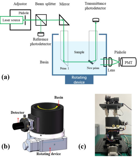
Figure 1.
(a) Schematic of the measurement principle of the VSF instrument. The wavelength of the laser source is 532 nm (as an alternative, the 520 nm CW laser module of MatchBoxTM is available). The pinhole is used to block the divergent stray light of the laser source. The adjustor is set for the adjustment of the laser source’s tilt angle. The beam splitter separates the laser into two beams: reflected beam and transmitted beam. The reflected beam is detected by the reference photodetector. The transmitted beam enters the sample via the mirror and prism 1, leaves the sample via the new prism, and is detected by the transmittance photodetector. Scattered light is detected by the photomultiplier tube (PMT) that spins along with the rotating device and basin. (b) Schematic of the rotatable component. The basin is used to store the sample where scattering occurs. The detector is rotated following the direction of the yellow arrow together with the basin driven by the rotating device. (c) Exhibition of VSFlab.
The basin is fixed on the rotating device, and the detector is installed at the wall of the basin. The scattering signal is collected by the detecting module, which includes the lens, pinhole, and PMT. A high-performance PMT (HAMAMATSU H10721-20) whose minimum detectable power is about 1.25 × 10⁻⁹ mW is used to meet the required dynamic range of nearly five orders of magnitude. The schematic of the rotatable component is shown in Figure 1b. The basin is used to store the sample where scattering occurs. The detector, together with the basin, spins under the drive of the rotating device. A complete measurement is not time consuming and typically lasts 8 s. The basin is oxidized and turned black to protect it from erosion and reduce the amount of stray light reflected from its wall. The assembled VSFlab is shown in Figure 1c.
2.2. Description of New Prism Design
The prism P2 used in POLVSM (Figure 2a) is a specially customized prism that creates an air gap to prevent reflected light from entering the basin. As the backward scattered light near 180° is weak and easily overestimated, creating an air gap is an important and necessary way to reduce stray light. However, in our practice, this structure is relatively expensive and tends to easily break during manufacturing. More importantly, making the top surface of this air gap smooth and flat enough in practice is a challenge because the polishing process is implemented via a small customized mold in a limited space where the checking process is difficult to carry out. Therefore, flaws likely occur, and light usually diffuses and brings undesired stray light.
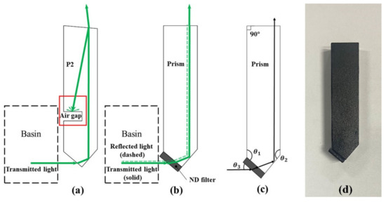
Figure 2.
Schematic of different prisms and angle design of new prism. (a) P2. An air gap, as shown in the red box, is created inside the prism to prevent the light reflected onto the top surface of the prism from going back to the basin. However, diffused light, represented by the short green arrows, easily occurs in practice at the surface of the air gap when the surface is not smooth. (b) Designed prism structure. The solid green line and dashed green line represent the transmitted light and reflected light, respectively. (c) Angle design of new prism. These angles (θ1, θ2, and θ3) make the transmitted light vertical to the surface of the prism. (d) The manufactured new prism.
For convenient manufacturing, we propose a relatively simple prism design, as shown in Figure 2b. The new prism sticks a single prism and an ND filter together instead of creating an air gap. The surfaces around the prism, except for the top surface, are coated with black paint, which has an absorption greater than 99.75%. The ND filter in this prism has a low transmittance of 1% and a surface roughness of 1/4 λ. Theoretically, the forward light intensity experiences a loss of at least 99% when the light propagates through the filter for the first time. Then, more than 98% of the transmitted forward light escapes from the top surface of the prism for c measurements, and only nearly 2% of the transmitted forward light is reflected back to the prism. This reflected light undergoes another loss of at least 99% when propagating the ND filter back to the basin. As the transmittance of the light passing through the ND filter is even lower than 1% because the filter is put aslant, the amount of reflected light back to the basin is much less than 10−6 of the forward light. To ensure that the interface between the ND filter and the prism is thin enough to guarantee good transmittance and negligible refraction, we use an interferometer in checking whether the surfaces of the ND filter and prism are polished such that their roughness reaches 1/4 λ. Benefiting from mature manufacturing and efficient optical glue, our ND filter and prism could be seamlessly integrated.
As this prism is designed to ensure that the transmitted light is vertical to the top surface of the prism for the correct measurement of c, the determination of each angle, including θ1, θ2, and θ3 marked in Figure 2c, follows Equation (4).
where represents the refractive index of the prism and represents the refractive index of the sample. An optical simulation is implemented in the TracePro simulation platform to verify the rationality of the prism design. The input light intensity is set to 1. For prism (b), the light reflected to the basin is almost 10−6. The transmitted light accepted by the photodetector is 0.0099. The simulation results show that the intensity of the stray light can be reduced to less than 10−6 of the forward beam. In this way, the reflected light exerts minimal influence on the backward scattered light. The manufactured new prism is shown in Figure 2d.
2.3. Data Correction and Calibration
To accurately obtain particulate VSF and evaluate the performance of the VSFlab, a series of work including correction and calibration were carried out. These processes were implemented in the laboratory based on samples of nearly monodisperse standard polystyrene spherical beads (Duke STANDARDSTM) from Thermo Fisher Scientific Inc., Waltham, MA, USA. As the standard particles are nearly perfectly spherical and their size distribution and refractive index have been correctly characterized by the manufacturers, their VSFs can be predicted with high accuracy by using Mie theory and thus provide a means to calibrate the functioning of the instrument. Mie theory considers: (1) wavelength of light; (2) particle size (mean size and size distribution); (3) size parameter, defined as x = 2πr/λ, where r and λ are the sphere radius and wavelength of light (in the medium surrounding the particle); (4) the complex index of refraction of the spheres (np = nr + ni) relative to the surrounding medium (nw), n = np/nw. The polystyrene beads used in this study are listed in Table 1. The real index of refraction for polystyrene was calculated based on the results of Ma et al. and we used a value of 0.00035 ± 0.00015 for the imaginary part of the refractive index [28]. The index of refraction of pure water at room temperature is 1.3368 at 520 nm and 1.3363 at 532 nm.

Table 1.
The specification of polystyrene beads used in this study. Beads of a nominal diameter μND are assumed to be normally distributed with an actual mean diameter of μD and a standard deviation of σD. σD represents the uncertainty in determining μD at 95% confidence level. The complex refractive index (n) at 532 nm and 520 nm are also listed.
2.3.1. Scattering Volume Correction and Angular Calibration
Scattering volume is defined as the volume illuminated by the incident beam, and it must be constant over all scattering angles for VSF measurements. However, it varies steadily with the scattering angle in a complex way. Scattering volume correction should thus be implemented. Scattering volume correction is performed following the method proposed by Chami et al. [23], who reported that the variation of scattering volume relative to the scattering volume at 90° (about 0.02 cm3 in this work) can be expressed as the inverse of a sine function.
Specifically, the consistency of the angular measurements was checked. When the rotating device is activated, acceleration occurs. To ensure a uniform rotation in the scattering angle range of 0°–180° and a uniformly spaced angle interval, we set the instrument so that it starts sampling before the scattering angle reaches 0°. Thus, the aim of angular calibration is to find the first and last sampling points and calibrate the angular discrepancy. Angular calibration was realized through VSF measurement on standard beads with a mean diameter of 2.0 µm suspended in water. The results for 2.0 µm beads showed a distinct pattern with several scattering maxima and minima due to the constructive and destructive interferences of the scattered light from a nearly monodisperse population of beads that are large relative to the light wavelength. Angular calibration can be achieved by assigning the detected VSF maxima or minima using a second-order polynomial curve fitting. Furthermore, 3, 5, and 11 µm beads are used for angular validation.
2.3.2. Baseline Measurement
In obtaining the VSFs of hydrosols, the methodology consists of performing measurements for a sample containing pure water only; such measurement is hereinafter referred to as “baseline measurement.” Performing this measurement is essential because the contribution for pure water (or pure sea water) βw(θ) to the total VSF β(θ) should be removed to allow the determination of particle contribution βp(θ).
When measuring VSF of standard beads, pure water was prepared by the Milli-Q advantage A10 water purification system (Millipore Inc., Burlington, MA, USA) and then filtered through a polycarbonate cartridge filter of pore size 0.2 μm (PN 12991, Pall Co. Ltd., Port Washington, NY, USA) to further remove residual particle contaminations. During offshore observations, the filtered seawater was prepared for baseline measurement. Additionally, a Liqui-Cel Membrane Contactor with a vacuum pump was used to remove the bubbles inside the pure water samples so as to obtain correct baseline measurements. Finally, these baseline measurements were subtracted from the subsequent measurements taken on particle suspensions.
2.3.3. Amplitude Calibration
The output voltage signal was calibrated by measuring the absolute magnitude of the VSF in m−1sr−1 of a standard bead solution, for which the scattering magnitude is known. The 0.203 µm beads were smaller than the wavelength of light, thus leading to the featureless shape of the VSF. By contrast, the large beads exhibited ripples in the angular scattering that made the calibration result highly sensitive to the angular acceptance of the detector. Following the suggestion of Hu et al. [29], we used small-sized beads with a nominal diameter of 0.203 µm for calibration and other large-sized beads for validation. Its attenuation coefficient c is equal to the scattering coefficient b and thus:
where is the scattering phase function obtained from Mie theory. The impact of the uncertainties (measured as the coefficient of variation) of 0.203 µm beads at 532 nm in the mean diameter varying within μD ± δD on is 3.4%. The imaginary part of the refractive index of 0.203 µm beads is small in the visible wavelengths and its effects on scattering could be neglected [21]. The calibration coefficient k(θ) is derived as the slope between the output signal after scattering volume correction Voltage (θ) and the βMie (θ) by applying the linear regression model.
The calibration coefficient k at each scattering angle was determined from the solutions with various concentrations of 0.203 µm beads. A 100 mL master solution of 0.203 µm beads with c of 7.5 m−1 was prepared and was agitated on a vortex mixer to homogenize the suspension and break down possible aggregation of particles. Subsequently, a certain amount (totally from 20 mL to 70 mL) of the master solution was added into the pure water (about 400 mL) in the basin, producing a series of solutions with c from 0.36 to 1.12 m−1. After each addition, the stirring rod was used to homogenize the beads in the basin before taking 30 measurements of the VSFs. The VSF measurements should be implemented within the single scattering regime to ensure the negligible effects of multiple scattering over the path length used by a given instrument. The criterion for a single scattering regime is defined in terms of small optical thickness, which is generally less than 0.1 [30]. The path length of VSFlab is 0.065 m; thus, c of the experimental samples used in our calibration procedure was kept under 1.54 m−1.
2.3.4. Validation of the Attenuation Measurement
The module of c measurement is set up so that the samples’ c and VSF can be measured simultaneously. The accuracy of c needs to be validated since (1) c is an indispensable parameter to determine the calibration coefficient k during amplitude calibration; (2) it is used for the correction of the attenuation of the primary beam and the scattered light.
A Perkin–Elmer (PE) Lambda 35 spectrophotometer was used to collect independent c measurements of the polystyrene beads suspended in water to validate the beam attenuation data from VSFLab. The c of the master solution was verified through this instrument. c was measured by placing a 1 cm sample quartz cuvette close to the output window of the sample beam and an additional custom cuvette with an aperture of 0.8 mm in front of the detector to reduce the acceptance angle of the detector to less than 0.23° [31,32]. A series of samples with different concentrations (c = 0.13 m−1, 0.55 m−1, 0.79 m−1, 1.33 m−1) of suspended 2.0 µm standard polystyrene beads were prepared. More than 30 measurements were taken on each sample to compare the measurements from VSFlab with those from PE Lambda 35. Comparison results that the R2 value and RMSE were 96.84% and 0.047 m−1, respectively indicated that the new prism yields good performance in the c measurements.
Then, the c measurements for each sample were applied to the correction of light attenuation along the pathway inside the scattering volume following the procedure proposed by Chami et al. [23]. As scattering measurements were acquired in a single scattering regime, the attenuation correction exerted a minor influence on the VSF measurements.
2.3.5. Calibration of LISST-VSF
LISST-VSF was used to validate the performance of VSFlab and its implementation of the automatic calibration was as follows. We cleaned the inner endcaps and the windows, drained the test chamber, wiped, and dried the windows. Then, baseline measurement was implemented to subtract the pure water from total scattering to determine the calibration coefficients. LISST-VSF was installed on the laboratory table according to the instructions as shown in Figure 3. The pre-filtered water was poured into the sample volume. The polycarbonate cartridge filter of pore size 0.2 μm (PN 12991, Pall Co. Ltd., New York, NY, USA), the diaphragm pump (Millipore Inc., Burlington, MA, USA), and the Liqui-Cel Membrane Contactor (Minnesota Mining and Manufacturing Co. Ltd., Decatur, AL, USA) were connected through silica gel tube to form a circulating system. Filtration and bubbles removal lasted for one hour. The degassed and particle-free water was prepared. The LISST-VSF ring data is sensitive to ambient light, so the sample volume was covered with an opaque rag during measurement.
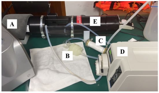
Figure 3.
Installation of LISST-VSF in lab. (A) represents the opaque rag. (B) represents the polycarbonate cartridge filter of pore size 0.2 μm. (C) represents the Liqui-Cel Membrane Contactor. (D) represents the diaphragm pump. (E) represents LISST-VSF. The polycarbonate cartridge filter of pore size 0.2 μm, the diaphragm pump, and the Liqui-Cel Membrane Contactor were connected through silica gel tube to form a filtration, degassing, and circulating system.
2.4. Field Observation
Two field observations including 21 stations were carried out in the East China Sea (ESC) in May 2021 and August 2021 (see Figure 4). The farthest station was about 90 km offshore. The filtered seawater was prepared for baseline measurement. To avoid the influence of ship shaking on the VSFlab, the angle and amplitude calibration of VSFlab were implemented every day. According to the c of samples, we diluted the samples to meet the requirements of single scattering. The samples were fully mixed in a magnetic stirrer before measurement. Since a complete measurement requires 8 s, it could be considered that the particles were evenly distributed in the solution during the measurement. Noting the influence of bubbles on the measurement results [33], we took extra care in the process of water collection, liquid transfer, and dilution to avoid bubbles as far as possible.
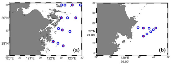
Figure 4.
All 21 Stations (blue circles) at the East China Sea (ESC) including 9 stations for microscopic imaging (red plus). (a) The observation in May 2021. (b) The observation in August 2021.The gray part represents the land and the white part represents the sea.
A particle sizer (BT-3000) manufactured by Dandong Bettersize Instruments Ltd. (Dandong, China) was utilized to analyze particle size and morphology. It is equipped with a microscope to carry out microscopic imaging of particles in the water ample. The circulation system ensures the full dispersion of the sample. Then, according to the image, it calculates the circle equivalent diameter to describe the particle size [34] and circularity, which considers the relationship between the shape area and the shape perimeter, to describe the degree of irregularity of particle shape [35]. Note that recording microscopic images of particles is time consuming, so we only took images of particles at nine stations which are marked as red plus symbols in Figure 3.
3. Results and Discussions
3.1. Calibration of VSFlab
To achieve the absolute magnitude of VSF in m−1 sr−1, in addition to baseline correction and angular calibration, we implemented amplitude calibration by utilizing solutions with various concentrations of 0.203 µm standard beads for the VSFlab at 532 nm. In this way, the calibration coefficient k at each scattering angle was determined. Figure 5a shows the correlation between the raw signal voltage and the theoretical VSF for the new prism at four scattering angles of 6°, 90°, 177°, and 178.5°. The high coefficients of determination R2 indicated that the calibration procedure was reliable. The estimated calibration coefficient k for each scattering angle is shown in Figure 5b. The angular distribution of k for both prisms was relatively smooth between 3° and 177°, with the average k being 65.1 ± 4.68 m−1 sr−1/V. Such characteristic was determined by the fact that the single detector used herein ensured the constant photoelectric conversion efficiency. Sharp increases were observed at scattering angles close to 0° and 180° (typically from <3° and >165°) because of the prism’s shadowing effect. As shown in Figure 5d, the scattering light at small angles close to 0° and 180° was shadowed by the prism, which limited the minimum and maximum detectable angles [23]. We applied the estimated calibration coefficient k to the measurements of 3.0 µm standard beads. It was found that such loss of light intensity due to the shadow effect could be compensated through amplitude calibration (Figure 5c). At scattering angles from 1° to 3° and from 177° to 178.5°, the significant underestimation of measured VSF was observed before the amplitude calibration based on the comparison with the theoretical one calculated from Mie theory. After the calibration, the VSF was more consistent with the theoretical curve in the two angle ranges. It indicated that our calibration procedure for the VSFlab was reasonable.
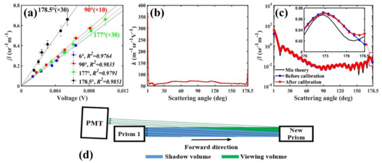
Figure 5.
(a) Scatterplot between raw signal voltage measured by VSFlab and calculated VSF for 0.203 μm bead solutions with various concentrations at four scattering angles of 6° (blue dots), 90° (red dots), 177° (green dots) and 178.5° (dark dots). The values (voltage and β) at 90°, 177°, and 178.5° are multiplied by 10, 30, and 30 for an unambiguous presentation. The four lines are the results of applying a robust linear regression model. R2 for the four angles are 0.9764, 0.9835, 0.9791, and 0.9851 respectively. Horizontal and vertical error bars represent standard deviations estimated, respectively, from the 30 measurements of Voltage (θ) at each concentration and calculated by accounting for uncertainties in the mean diameter of the beads and measured c. (b) Calibration coefficients k for each angle at 532 nm. (c) Comparison of VSFs for 3 μm beads before amplitude calibration and after amplitude calibration. In order to facilitate comparison with the calibrated scattering signal, the scattering signal before calibration was multiplied by the average k between 3° and 177°. (d) A schematic of the shadow effect. The blue region represents the scattering volume from which the scattering light is shadowed by prism 1. The green region represents the scattering volume from which the scattering light is received by the PMT.
3.2. Validation of the VSFlab and Comparison with LISST-VSF
To further validate our improvement on measurement of backward scattering, experiments on various sizes of polystyrene beads at 532 nm and 520 nm were carried out. Calibration for the VSFlab at 520 nm had been done using the same method mentioned in Section 2.3.
The phase function for 3 μm polystyrene beads at 532 nm was obtained according to Equation (3) for the comparison with POLVSM measurement which was redrawn from Chami’s work [23] and Mie theory calculated result (see Figure 6). Both results of VSFlab and POLVSM showed good agreement with Mie theory in 1° to 170°. Notable differences were observed in the backward scattering range between 170° and 178.5° (see Figure 6b), that the VSFlab result was closer to the theoretical result while the POLVSM result showed overestimations. The mean relative errors between 170° and 178.5° were 56.76% and 16.53% for POLVSM and VSFlab results, respectively. VSF results for 2, 5, and 11 μm polystyrene beads at 520 nm also revealed good agreement with theoretical results from 170° to 178.5° (see Figure 7d–f). The mean relative errors from 170° to 178.5° for 2, 5, and 11 μm beads were 21.5%, 45.3%, and 34.07%, respectively. It indicated that the customized new prism could reduce the stray light returning to the basin efficiently and such design could avoid manufacturing flaws.
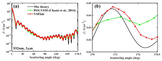
Figure 6.
(a) Comparison of phase functions for 3 μm beads at 532 nm obtained from the VSFlab (red line), redrawn from Chami’s work (green line) and calculated by Mie theory (black line). (b) Same as (a) but for angles between 170° and 178.5°.
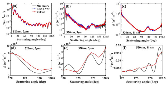
Figure 7.
(a–c) VSFs for 2, 5, and 11 μm beads at 520 nm. The blue line denotes the results measured by LISST-VSF, and the red line denotes the results measured by VSFlab. The black line corresponds to the theoretical curves calculated from Mie theory. (d–f) Same as (a–c) but for angles between 170° and 178.5°.
At the scattering angles between 1° and 150°, VSFlab was proved to be workable by comparison with LISST-VSF (see Figure 7a–c). The mean relative percentage difference of 2 μm polystyrene beads between VSF measured by LISST-VSF and theoretical values was 11.4% from 1° to 150° and that between VSF measured by VSFlab and theoretical values was 9.8% from 1° to 178.5°. For 5 and 11 μm polystyrene beads, the magnitude of the minima or maxima from VSFlab differed by a few tens of percent from the Mie scattering values. These deviations were due to the large angular acceptance of the detector in VSFlab relative to that in LISST-VSF. However, the angular acceptance of VSFlab was acceptable since the VSFs of the natural samples usually show smoother angular distributions, which could be confirmed in experimental results on natural samples. All these validations fully proved the reliability of our VSFlab in measuring the VSFs in the backward direction of 1° to 178.5°.
3.3. Observation Results in the ECS
3.3.1. VSF between 1° and 178.5°
The VSFlab instrument was used in several cruises to carry out the VSF measurements in the ECS. The VSFs in the ESC are shown in Figure 8a. The derived from measured VSF was 1.25–2.83%. The c of all measured samples ranged from 0.62 m−1 to 5.79 m−1. The chlorophyll concentration ranged from 0.27 to 53.06 mg/m3. For samples with c greater than 1.5 m−1, the water samples were diluted in advance to meet the requirement of single scattering.
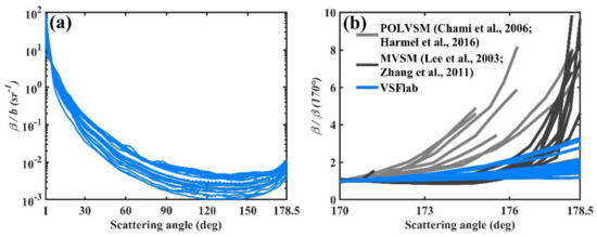
Figure 8.
(a) Phase functions at 532 nm between 1° and 178.5° in the ECS. (b) Comparison of VSFs at 532 nm measured by VSFlab, POLVSM and MVSM between 170° and 178.5°. All these VSFs were normalized at 170°.
The VSFs showed strong forward scattering. Forward and backward scattering differed by nearly five orders of magnitude. Past and recent studies about VSFs measurements that were performed in natural waters [13,36,37], showed a significant increase in the VSF in the backward direction at angles greater than 150°. However, only a few instruments, such as POLVSM and MVSM, yielded the VSF measurements at the angles greater than 170° [21,23,38,39], and there was large variability of VSF in this angle range. More than one order of magnitude increase in VSF from 170° to near 180° was sometimes observed. Hence, the comparison of the VSFs in the ECS with the results measured by POLVSM and MVSM at angles greater than 170° was made, which is shown in Figure 8b.
POLVSM has been used to measure various types of VSFs including dust and algae. The measured VSFs increased by an average of five times at angles larger than 170° [23,39]. The VSFs observed from MVSM in surface waters off the New Jersey coast showed even more increase by an average of 6.5 times, and the maximum growth exceeded 9.8 times [21,38]. A field experiment in the northern Adriatic Sea indicated that the VSF measurements by the MVSM at angles > 175 are unreliable due to stray light contamination and/or difficulty in precisely calculating the scattering volume [40]. Therefore, it can be further found that the VSFs from VSFlab and MVSM were in good agreement with the range of 170° to 175°, while a significant deviation was observed at an angle greater than 175°. Different from other VSFs, the VSFs in the ESC increased relatively slowly from 170° to 178.5°, about 1.24–3.97 times with an average of 2.19 times. In general, a moderate increase in VSFs at angles larger than 170° in the ECS was observed for the first time.
3.3.2. Variation of the χp Factor
The χp factor, defined as χp = bbp/(2πβp(θ)), is an important factor relating bbp with the particulate VSF measured at a single scattering angle and describing the shape of the particulate VSF in the backward direction [41,42,43]. Figure 9a shows the angular variation of the χp factor using VSFlab data from all sites of the ECS. Similar to results measured in other coastal and oceanic areas, χp of the ECS exhibited an increase from 90° to 120°, a relatively flat shape at angles of 120° to 150° and an obvious decrease at angles greater than 150°. The average and standard deviations (σ) of χp from all sites are shown in Figure 9b. The variability in χp was found to be less than 6% for most scattering angles within 90°–155°. The average of χp at 120° from the results in the ECS was 1.13 ± 3.81%. Other mean χp near 120° reported by Oishi et al. [42], Boss et al. [43], Zhang et al. [44], Sullivan et al. [36] and Berthon et al. [40] were 1.14 ± 10%, 1.12 ± 4.2%, 1.1 ± 1.45%, 1.097 ± 2.92%, and 1.1 ± 3.64%, respectively. Our result was very consistent with them. Another average of χp at 140° in the ECS was 1.21 ± 4.63%. Compared with other studies (χp(140°) = 1.18 ± 3.5%, 1.167 ± 4.2%, and 1.15 ± 3.48%) [36,40,43], our χp(140°) was only slightly higher. The conclusion proposed by Sullivan et al. that the estimates of the particulate backscattering coefficient using single angle scattering measurements near 120° or 140° and suitable conversion factors [36], was justified in the ECS.
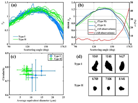
Figure 9.
(a) χp of two types of water from 90° to 178.5°. (b) Average χp (black line) and relative standard deviation for all observations (red line) from 90° to 178.5°. The blue and green lines represent mean χp of type I and II, respectively. (c) Scatter plot between degree of circularity and mean equivalent diameter. (d) Microscopic images of typical particles taken by BT-3000. The unit is micron.
Large variability in χp factors could be observed at angles greater than 155°, particularly greater than 170° (near 25%). Such large variability at 170° was also pointed out by Whitmire et al. [45], according to χp of thirteen different algae, but few studies have given the variability of χp after 170°. Our results showed that the variability increased with the angle after 155° and reached the maximum value of 42.3% at 178.5°. Based on the different backscattering shapes at angles greater than 155°, the VSFs measured in the ECS can be roughly classified into two types (type I and type II, see Figure 9). χp of type I and type II was close between 90° and 155°, but χp of type I was smaller than that of type II after 155°. The mean χp for the two types and all observations are presented in Figure 9b, indicating that the most difference between these two types occurred at angles after 170°. Such obvious deviation was closely associated with the particle size distribution, shape, and the real bulk index of refraction of the particles [46,47,48]. With the assistance of the BT-3000 micro imaging function, it could be found that the particles in type I and type II water had significant differences in particle size and morphology (see Figure 9c,d and Table 2). In terms of particle size, the average equivalent diameter of particles in type I samples (>10 μm) was obviously greater than that of type II (near 8 μm), and additionally, according to the σ calculation, type I samples had wider size distributions indicating that particles in these samples were more polydispersed. Another significant difference between the two types was found in the circularity of particles, that type I samples contained more irregular shapes particles while particles in type II samples were closer to spherical. These results confirmed that the high variability of χp in the near-backward direction was the result of high variability for various particles characteristics, not a reflection from inside the chamber of the instrument. Therefore, the variability of χp had a large potential to characterize the particles in the ECS.
Table 2.
Average, standard deviation (σ), and percent variability (σ as %) of equivalent diameter and circularity from the microscopic imaging analysis data of particles in water samples.
4. Conclusions
A VSF meter (VSFlab) was established and achieved good backward volume scattering function between 1° and 178.5° with the novel prism that prevents the stray light induced by the specular reflection of the incident beam from re-entering the scattering volume. A rigorous calibration method and validation for the VSFlab instrument converted the output raw signal into geophysical units (i.e., m−1 sr−1) and corrected the underestimation caused by the shadow effect of the prism. By comparison with Chami’s POLVSM measurement, which was redrawn from his work and Mie theory calculated results, the new prism was proved to be workable in reducing stray light. Furthermore, the VSF results for 2, 5, and 11 μm polystyrene beads at 520 nm were also in good agreement with the theoretical results. All these validations fully proved the reliability of VSFlab in measuring the VSFs.
Field observations in the East China Sea exhibited a moderate increase in VSFs from 170° to 178.5°, not more than five times, while the VSF results in other regions showed a relatively sharp increase. The measured VSF could provide a basis for the parameterization of VSF in the radiative transfer model. The variability of χp factors increased with an angle larger than 155° and reached the maximum value of 42.3% at 178.5°. Based on the different VSF shapes at angles greater than 155°, two types of VSFs were found in the ECS. With the assistance of BT-3000, it could be found that these two types differed in particle size distribution and shape parameters. The variability of χp in the backward direction has the potential to be used to characterize the particles in the ECS.
Author Contributions
Conceptualization, C.W. and B.T.; methodology, C.W. and B.T.; software, C.W. and B.T.; validation, C.W. and B.T.; formal analysis, C.W. and B.T.; investigation, C.W. and B.T.; resources, H.H., D.P. and Z.M.; data curation, Y.G. and H.S.; writing—original draft preparation, C.W. and B.T.; writing—review and editing, C.W. and B.T.; visualization, Y.G.; supervision, H.H., D.P. and Z.M.; project administration, H.H., D.P. and Z.M.; funding acquisition, B.T., D.P. and Z.M. All authors have read and agreed to the published version of the manuscript.
Funding
This research was funded by “The Key Special Project for Introduced Talents Team of Southern Marine Science and Engineering Guangdong Laboratory (Guangzhou), grant number GML2019ZD0602”; “the Scientific Research Fund of the Second Institute of Oceanography, SOA, grant number QNYC201602”; “the National Natural Science Foundation of China, grant number 41876033 and 61991454”.
Institutional Review Board Statement
Not applicable.
Informed Consent Statement
Informed consent was obtained from all subjects involved in the study. Written informed consent has been obtained from the patient(s) to publish this paper.
Data Availability Statement
Not applicable.
Acknowledgments
We thank Yaorui Pan, Changpeng Li and Youzhi Li from the second institution of oceanography for help carrying out experiments for this work.
Conflicts of Interest
The authors declare no conflict of interest.
References
- Mobley, C.D.; Sundman, L.K.; Boss, E. Phase function effects on oceanic light fields. Appl. Opt. 2002, 41, 1035–1050. [Google Scholar] [CrossRef] [Green Version]
- Duntley, S.Q. Light in the Sea*. J. Opt. Soc. Am. 1963, 53, 214–233. [Google Scholar] [CrossRef]
- Sokolov, A.; Chami, M.; Dmitriev, E.; Khomenko, G. Parameterization of volume scattering function of coastal waters based on the statistical approach. Opt. Express 2010, 18, 4615–4636. [Google Scholar] [CrossRef] [PubMed]
- Slade, W.H.; Boss, E.S. Calibrated near-forward volume scattering function obtained from the LISST particle sizer. Opt. Express 2006, 14, 3602–3615. [Google Scholar] [CrossRef] [PubMed]
- Chami, M.; McKee, D.; Leymarie, E.; Khomenko, G. Influence of the angular shape of the volume-scattering function and multiple scattering on remote sensing reflectance. Appl. Opt. 2006, 45, 9210–9220. [Google Scholar] [CrossRef]
- McLeroy-Etheridge, S.L.; Roesler, C.S. Are the inherent optical properties of phytoplankton responsible for the distinct ocean colors observed during harmful algal blooms? Ocean Opt. 1998, 14, 109–116. [Google Scholar]
- Dall’Olmo, G.; Westberry, T.; Behrenfeld, M.; Boss, E.; Slade, W. Significant contribution of large particles to optical backscattering. Biogeosciences 2009, 6, 947–967. [Google Scholar] [CrossRef] [Green Version]
- Hubert, L.; Lubac, B.; Dessailly, D.; Duforet-Gaurier, L.; Vantrepotte, V. Effect of inherent optical properties variability on the chlorophyll retrieval from ocean color remote sensing: An in situ approach. Opt. Express 2010, 18, 20949–20959. [Google Scholar] [CrossRef]
- Gordon, H.R.; Brown, O.B.; Jacobs, M.M. Computed Relationships Between the Inherent and Apparent Optical Properties of a Flat Homogeneous Ocean. Appl. Opt. 1975, 14, 417–427. [Google Scholar] [CrossRef]
- Tyler, J.E.; Richardson, W.H. Nephelometer for the Measurement of Volume Scattering Function in Situ. J. Opt. Soc. Am. 1958, 48, 354–357. [Google Scholar] [CrossRef]
- Tyler, J.E. Scattering Properties of Distilled and Natural Waters. Limnol. Oceanogr. 1961, 6, 451–456. [Google Scholar] [CrossRef]
- Kullenberg, G. Scattering of Light by Sargasso Sea Water. Deep. Sea Res. Oceanogr. Abstr. 1968, 15, 423–432. [Google Scholar] [CrossRef]
- Petzold, T.J. Volume Scattering Functions for Selected Ocean Waters; Scripps Institution of Oceanography: San Diego, CA, USA, 1972. [Google Scholar]
- Reuter, R. Characterization of marine particles suspensions by light scattering (II). Experimental results. Oceanol. Acta 1980, 3, 325–332. [Google Scholar]
- Kullenberg, G. Observations of light scattering functions in two oceanic areas. Deep Sea Res. Part A Oceanogr. Res. Pap. 1984, 31, 295–316. [Google Scholar] [CrossRef]
- Jonasz, M. Volume Scattering Function Measurement Error Effect of Angular Resolution of the Nephelometer. Appl. Opt. 1990, 29, 64–70. [Google Scholar] [CrossRef]
- Volten, H.; Haan, J.F.; Hovenier, J.W.; Schreurs, R.; Vassen, W.; Dekker, A.G.; Hoogenboom, H.J.; Charlton, F.; Wouts, R. Laboratory measurements of angular distributions of light scattered by phytoplankton and silt. Limnol. Oceanogr. 1998, 43, 1180–1197. [Google Scholar] [CrossRef]
- Lotsberg, J.K.; Marken, E.; Stamnes, J.J.; Erga, S.R.; Aursland, K.; Olseng, C. Laboratory measurements of light scattering from marine particles. Limnol. Oceanogr. Methods 2007, 5, 34–40. [Google Scholar] [CrossRef]
- Zugger, M.E.; Messmer, A.; Kane, T.J.; Prentice, J.; Concannon, B.; Laux, A.; Mullen, L. Optical scattering properties of phytoplankton: Measurements and comparison of various species at scattering angles between 1° and 170°. Limnol. Oceanogr. 2008, 53, 381–386. [Google Scholar] [CrossRef] [Green Version]
- Svensen, O.; Stamnes, J.J.; Kildemo, M.; Aas, L.M.; Erga, S.R.; Frette, O. Mueller matrix measurements of algae with different shape and size distributions. Appl. Opt. 2011, 50, 5149–5157. [Google Scholar] [CrossRef]
- Lee, M.E.; Lewis, M.R. A new method for the measurement of the optical volume scattering function in the upper ocean. J. Atmos. Ocean. Technol. 2003, 20, 563–571. [Google Scholar] [CrossRef]
- Shao, B.; Jaffe, J.S.; Chachisvilis, M.; Esener, S.C. Angular resolved light scattering for discriminating among marine picoplankton-modeling and experimental measurements. Opt. Express 2006, 14, 12473–12484. [Google Scholar] [CrossRef] [PubMed]
- Chami, M.; Thirouard, A.; Harmel, T. POLVSM (Polarized Volume Scattering Meter) instrument: An innovative device to measure the directional and polarized scattering properties of hydrosols. Opt. Express 2014, 22, 26403–26428. [Google Scholar] [CrossRef] [PubMed]
- Li, C.; Wenxi, C.; Yu, J.; Ke, T.; Lu, G.; Yang, Y.; Guo, C. An Instrument for In Situ Measuring the Volume Scattering Function of Water Design Calibration and Primary Experiments. Sensors 2012, 12, 4514–4533. [Google Scholar] [CrossRef] [PubMed]
- Liao, R.; Roberts, P.L.; Jaffe, J.S. Sizing submicron particles from optical scattering data collected with oblique incidence illumination. Appl. Opt. 2016, 55, 9440–9449. [Google Scholar] [CrossRef] [PubMed]
- Wanyan, W.; Kecheng, Y.; Man, L.; Wenping, G.; Min, X.; Wei, L. Measurement of Three-Dimensional Volume Scattering Function of Suspended Particles in Water. Acta Opt. Sin. 2018, 38, 11. [Google Scholar]
- Slade, W.H.; Agrawal, Y.C.; Mikkelsen, O.A. Comparison of Measured and Theoretical Scattering and Polarization Properties of Narrow Size Range Irregular Sediment Particles. In Proceedings of the Oceans-IEEE, San Diego, CA, USA, 23–27 September 2013. [Google Scholar]
- Ma, X.; Lu, J.Q.; Brock, R.S.; Jacobs, K.M.; Yang, P.; Hu, X.H. Determination of complex refractive index of polystyrene microspheres from 370 to 1610 nm. Phys. Med. Biol. 2003, 48, 4165–4172. [Google Scholar] [CrossRef]
- Hu, L.; Zhang, X.; Xiong, Y.; He, M.X. Calibration of the LISST-VSF to derive the volume scattering functions in clear waters. Opt. Express 2019, 27, A1188–A1206. [Google Scholar] [CrossRef] [Green Version]
- Hulst, H.C.; van de Hulst, H.C. Light Scattering by Small Particles; Dove Publications Inc.: New York, NY, USA, 1957. [Google Scholar]
- Morel, A.; Bricaud, A. Inherent optical properties of algal cells including picoplankton: Theoretical and experimental results. Can. Bull. Fish. Aquat. Sci. 1986, 214, 521–559. [Google Scholar]
- Stramski, D.; Babin, M.; Wozniak, S.B. Variations in the optical properties of terrigenous mineral-rich particulate matter suspended in seawater. Limnol. Oceanogr. 2007, 52, 2418–2433. [Google Scholar] [CrossRef] [Green Version]
- Zhang, X.D.; Lewis, M.; Johnson, B. Influence of bubbles on scattering of light in the ocean. Appl. Opt. 1998, 37, 6525–6536. [Google Scholar] [CrossRef]
- Coutinho, Y.A.; Rooney, S.C.K. and Payton, E.J. Analysis of EBSD Grain Size Measurements Using Microstructure Simulations and a Customizable Pattern Matching Library for Grain Perimeter Estimation. Metall. Mater. Trans. A 2017, 48, 2375–2395. [Google Scholar] [CrossRef]
- Xiao, B.; Wang, G. Shape circularity measure method based on radial moments. J. Electron. Imaging 2013, 22, 033022. [Google Scholar] [CrossRef]
- Sullivan, J.M.; Twardowski, M.S. Angular shape of the oceanic particulate volume scattering function in the backward direction. Appl. Opt. 2009, 48, 6811–6819. [Google Scholar] [CrossRef]
- Tan, H.; Doerffer, R.; Oishi, T.; Tanaka, A. A new approach to measure the volume scattering function. Opt. Express 2013, 21, 18697–18711. [Google Scholar] [CrossRef]
- Zhang, X.; Twardowski, M.; Lewis, M. Retrieving composition and sizes of oceanic particle subpopulations from the volume scattering function. Appl. Opt. 2011, 50, 1240–1259. [Google Scholar] [CrossRef]
- Harmel, T.; Hieronymi, M.; Slade, W.; Rottgers, R.; Roullier, F.; Chami, M. Laboratory experiments for inter-comparison of three volume scattering meters to measure angular scattering properties of hydrosols. Opt. Express 2016, 24, A234–A256. [Google Scholar] [CrossRef] [Green Version]
- Berthon, J.F.; Shybanov, E.; Lee, M.E.; Zibordi, G. Measurements and modeling of the volume scattering function in the coastal northern Adriatic Sea. Appl. Opt. 2007, 46, 5189–5203. [Google Scholar] [CrossRef]
- Maffione, R.A.; Dana, D.R. Instruments and methods for measuring the backward-scattering coefficient of ocean waters. Appl. Opt. 1997, 36, 6057–6067. [Google Scholar] [CrossRef]
- Oishi, T. Significant Relationship Between the Backward Scattering Coefficient of Sea-Water and the Scatterance at 120-Degrees. Appl. Opt. 1990, 29, 4658–4665. [Google Scholar] [CrossRef]
- Boss, E.; Pegau, W.S. Relationship of light scattering at an angle in the backward direction to the backscattering coefficient. Appl. Opt. 2001, 40, 5503–5507. [Google Scholar] [CrossRef]
- Zhang, X.D.; Boss, E.; Gray, D.J. Significance of scattering by oceanic particles at angles around 120 degree. Opt. Express 2014, 22, 31329–31336. [Google Scholar] [CrossRef]
- Whitmire, A.L.; Pegau, W.S.; Karp-Boss, L.; Boss, E.; Cowles, T.J. Spectral backscattering properties of marine phytoplankton cultures. Opt. Express 2010, 18, 15073–15093. [Google Scholar] [CrossRef] [Green Version]
- Meyer, R.A. Light-Scattering from Biological Cells—Dependence of Backscatter Radiation on Membrane Thickness and Refractive-Index. Appl. Opt. 1979, 18, 585–588. [Google Scholar] [CrossRef]
- Bohren, C.F.; Singham, S.B. Backscattering by Nonspherical Particles—A Review of Methods and Suggested New Approaches. J. Geophys. Res.-Atmos. 1991, 96, 5269–5277. [Google Scholar] [CrossRef]
- Stramski, D.; Boss, E.; Bogucki, D.; Voss, K.J. The role of seawater constituents in light backscattering in the ocean. Prog. Oceanogr. 2004, 61, 27–56. [Google Scholar] [CrossRef]
Publisher’s Note: MDPI stays neutral with regard to jurisdictional claims in published maps and institutional affiliations. |
© 2022 by the authors. Licensee MDPI, Basel, Switzerland. This article is an open access article distributed under the terms and conditions of the Creative Commons Attribution (CC BY) license (https://creativecommons.org/licenses/by/4.0/).