Fresher Experience Plays a More Important Role in Prioritized Experience Replay

Abstract

Prioritized experience replay (PER) is an important technique in deep reinforcement learning (DRL). It improves the sampling efficiency of data in various DRL algorithms and achieves great performance. PER uses temporal difference error (TD-error) to measure the value of experiences and adjusts the sampling probability of experiences. Although PER can sample valuable experiences according to the TD-error, freshness is also an important character of experiences. It implicitly reflects the potential value of experiences. Fresh experiences are produced by virtue of the current networks and they are more valuable for updating the current network parameters than the past. The sampling of fresh experiences to train the neural networks can increase the learning speed of the agent, but few algorithms can perform this job efficiently. To solve this issue, a novel experience replay method is proposed in this paper. We first define that the experience freshness is negatively correlated with the number of replays. A new hyper-parameter, the freshness discounted factor $\mu$, is introduced in PER to measure the experience freshness. Further, a novel experience replacement strategy in the replay buffer is proposed to increase the experience replacement efficiency. In our method, the sampling probability of fresh experiences is increased by raising its priority properly. So the algorithm is more likely to choose fresh experiences to train the neural networks during the learning process. We evaluated this method in both discrete control tasks and continuous control tasks via OpenAI Gym. The experimental results show that our method achieves better performance in both modes of operation.

1. Introduction

Deep reinforcement learning (DRL) enables resolution of the complicated decision-making tasks due to the combination of reinforcement learning (RL) and deep learning (DL). The idea of DRL is derived from behavioural psychology, which is mainly opted for most appropriate behavior in a given environment. For instance, Sutton defines RL as finding the best matches between the states and actions by trial-and-error in order to obtain the maximum of long-term cumulative rewards [1]. So far, DRL has already acquired remarkable achievements in AlphaGo [2], Atari games [3], Robotics [4,5,6], etc., because of the powerful self-learning capability. With the advent of artificial intelligent, DRL also has been applied in many different fields: finance [7,8,9], healthcare [10,11] and smart grid [12,13,14].

In standard RL algorithms [15,16], the experiences for updating the internal beliefs are discarded immediately, which in turn reduces both data usage and computation efficiency. In this case, experience replay (ER) [17] stores the experiences in a memory buffer of certain size to address this problem precisely; the agent interacts with the environment, and the experiences can be retrieved into the buffer. After the buffer is full, the latest experience takes the place of the oldest one. At each step, a random batch of experiences is sampled from the buffer to update the parameters of the agent. The application of ER can break the temporal correlations of data, thereby the data usage efficiency increases. On account of the great benefit of ER, it is widely used in all kinds of DRL algorithms [18].

Typical model-free DRL algorithms, such as deep Q-learning [18,19,20,21], policy gradient [22,23,24], deterministic policy gradient [25,26], distributional RL [27,28], etc., have been drawing attention. Of these, deep Q-networks (DQN) [18] utilizes the neural networks to approximate action-value function $Q(s,a)$. It has the advantage of learning control policies from high-dimensional input and can obtain human comparable performance in Atari games. Following the success, many variants of DQN have been invented to the appeared problems in DQN. For instance, double DQN [19], which is devoid of additional networks or parameters, can effectively address the problem e.g., the action-value function $Q(s,a)$ is highly overestimated in Q-learning. Dueling DQN [20] decouples value and advantage in DQN through dueling architecture, which eases the ability to learn state-value function $V\left(s\right)$ more efficiently. The aforementioned algorithms can only be applied in discrete control tasks, however, most physical control tasks have continuous action spaces. Recently, many algorithms have been proposed to deal with this issue. Deep Deterministic Policy Gradient (DDPG) [25], which uses deep function approximators, can learn policies in continuous action spaces. Twin Delayed Deep Deterministic policy gradient (TD3) [26] builds on double Q-learning. It takes the minimum value between a pair of critics to limit overestimation and propose delaying policy updates to reduce per-update error. TD3 greatly improves both the learning speed and performance of DDPG.

Moreover, the application scenarios of DRL have been becoming more complex; the traditional ER algorithm is not efficient due to uniform sampling. The experiences sampled from the replay buffer are of great significance to improve the efficiency of DRL algorithms, as the action-value function $Q(s,a)$ is directly learned from the samples. The experiences are feedback of the environment to the agent, which inform the agent whether the current action is good or not. So, it is crucial to find an efficient way to sample the experiences. Prioritized Experience Replay (PER) [29] is proposed to assign the experiences priority according to the absolute value of temporal difference error (TD-error), where a larger absolute TD-error denotes higher priority. Hence, the agent is more likely to replay important experiences instead of uniformly choosing experiences from the replay buffer. In addition, Combined Experience Replay (CER) [30] is a modification of PER. It considers the freshness of experiences and always puts the latest experience into the mini-batch to train the neural network. Of note, fresh experiences are produced by virtue of the current networks i.e., they are more valuable for updating current network parameters than the past. In other words, the learning speed of the agent can increase as long as the sampled experiences are fresh enough. Unfortunately, this fact has been neglected by the community for a long time.

In light of the above-mentioned issues, this paper focuses on the freshness of all experiences in the replay buffer instead of the latest one. Our objective is to figure out how the experience freshness affects the learning process of DRL. To be more concrete, a freshness discounted factor $\mu$ is introduced for the process of calculating the experience priority. This method can decrease the priority of past experiences by recording the replay times of experiences. Therefore, the sampling probability of fresh experiences can enhance indirectly. The major contributions of this paper are summarized as follows:

• Evaluation of Freshness. A freshness discounted factor $\mu$ is introduced evaluate the freshness of each experience during the calculation of the priority of each experience. The constraint of $\mu$ increases sampling probability of the fresher experience. We refer to this method as freshness prioritized experience replay (FPER) in the rest of this paper.
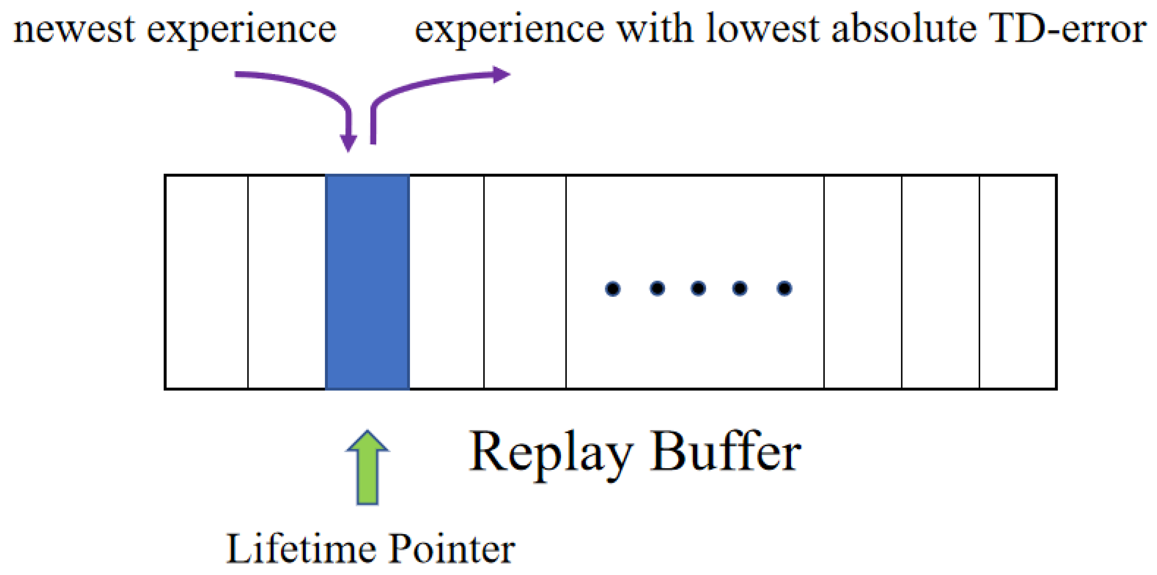
• Lifetime Pointer. In order to make the learning process more stable and to accelerate the convergence process, a lifetime pointer scheme is proposed. The pointer always points to the position of the experience with the lowest absolute TD-error. When the latest experience enters the buffer, it overwrites on the position pointed by the lifetime pointer. It prolongs the lifetime of valuable experiences, reduces the lifetime of worthless experiences, and further breaks the data correlation.

The mentioned FPER is not a complete DRL algorithm; it should be combined with other algorithms to form a complete learning system. In the experiments, we consider the combination of FPER with Dueling DQN and DDPG separately to validate its superiority in both discrete control tasks(e.g., CartPole-v1, LunarLander-v2) and continuous control tasks(e.g., HalfCheetah-v1, Ant-v1).

2. Related Work

PER is an important technique in DRL algorithms. In this section, we summarize some excellent papers about PER, which can distinguish improvements to PER from different perspectives. Results show that the reported contributions are very meaningful.

Based on the theoretical study on the influence of the size of the replay buffer by Liu et al. [31], Zhang and Sutton [30] propose CER to remedy the negative influence of a large replay buffer. As mentioned above, CER always puts the latest experience to the mini-batch and can learn the latest information and converge faster in case of large replay buffer. In other words, fresh information is more valuable. CER makes full use of this information to speed up the learning process. However, the improvement of one experience is limited while the complexity of the environment and the volume of mini-batch increase. On the other hand, CER’s performance restricts further if the replay buffer size is set properly [30]. This is clarified in Section 5.

Hou et al. [32] extend the application of PER from discrete control tasks to continuous control tasks. They combine DDPG with PER and point out that this practice can significantly reduce the training time of the network, improve the stability of the learning process, and strengthen the robustness of the model.

Based on this extension, Shen et al. [33] propose a classification mechanism (CLA) as an addition to PER. CLA contains a segmentation mechanism and a classification-swap mechanism. These mechanisms can swap the positions of two experiences in the same segment to preserve the experience with high absolute TD-error and can change the lifetimes of experiences in the buffer. However, CLA contains noticeable shortcomings. Although the swap procedure only costs $O\left(1\right)$ computations, the sorting procedure in the segmentation mechanism still costs $O\left(n^2\right)$ or $O\left(nlogn\right)$ computations. These additional computations could decrease the convergence rate. Moreover, the experiences in the same segment are similar due to their similar TD-errors, resulting in inefficient swap procedure. Intuitively, an experience with a low absolute TD-error should be replaced by an experience with high absolute TD-error.

3. Methodology

3.1. Dueling DQN and DDPG

In RL, the interaction process between the agent and environment is usually formulated as a Markov Decision Process (MDP). MDP is defined as a four-element tuple$(S,A,R,P)$, where S—state space, A—action space, R—reward function, and P—transition probability. The goal of RL is to learn the optimal policy ${\pi }^{*}$ which defines the agent’s behaviour and to maximize the discounted accumulative reward. The discounted accumulative reward function $G_t$ is given as:

$$G_t=R_t+\gamma R_{t+1}+{\gamma }^2{R}_{t+2}+\dots =\sum _{k=0}^{\infty }{\gamma }^k{R}_{t+k},$$

(1)

where $\gamma$ is the discounted factor determining the priority of short-term reward, and t is the time step.

The action-value function $Q^{\pi }(s,a)$ represents the expected reward after taking an action a in state s and following policy $\pi$:

$$Q^{\pi }(s,a)={\mathbb{E}}_{\pi }\left[G_t\mid S_t=s,A_t=a\right]={\mathbb{E}}_{\pi }\left[\sum _{k=0}^{\infty }{\gamma }^k{R}_{t+k}\mid S_t=s,A_t=a\right].$$

(2)

According to the Bellman Equation [34], $Q^{\pi }(s,a)$ can be expressed as an recursive formulation:

$$Q^{\pi }\left(s,a\right)={\mathbb{E}}_{\pi }\left[R_t+\gamma Q^{\pi }\left(S_{t+1},A_{t+1}\right)\mid S_t=s,A_t=a\right].$$

(3)

The action-value function in Dueling DQN [20] is calculated by two parts: value function $V\left(s\right)$ and advantage function $A(s,a)$. Let $\varphi$ denote the parameters of the convolutional layers, ${\varphi }_1$ and ${\varphi }_2$ are the parameters of two streams of fully-connected layers, respectively. To address the identifiability problem that V and A can not be inferred from Q, we have

$$Q(s,a;\varphi ,{\varphi }_1,{\varphi }_2)=V(s;\varphi ,{\varphi }_2)+\left(A(s,a;\varphi ,{\varphi }_1)-\frac{1}{\left|\mathcal{A}\right|}\sum _{a^{\prime }}A(s,a^{\prime };\varphi ,{\varphi }_1)\right).$$

(4)

Herein, the action space is discrete, Dueling DQN can indirectly achieve the optimal policy ${\pi }^{*}$ by searching all the action-value functions, which can be expressed as:

$${\pi }^{*}=arg\underset{\pi }{max}{Q}^{\pi }(s,a;\varphi ,{\varphi }_1,{\varphi }_2).$$

(5)

DDPG [25] cannot fit to the above approach due to the infinity of action space. It directly learns the optimal policy ${\pi }^{*}$. It contains two deep neural networks: the action-value network $Q(s,a,w)$ and the actor network $\pi (s,v)$. This two networks are used to approximate the action-value function $Q(s,a)$, as well as the actor function $\pi \left(s\right)$, respectively where w and v are the network parameters. The action-value network is to minimize the loss function $L\left(w\right)$, which is expressed as:

$$L\left(w\right)={\left(R_t+\gamma Q^{\prime }\left(S_{t+1},A_{t+1},w^{\prime }\right)-Q\left(S_t,A_t,w\right)\right)}^2,$$

(6)

Note: $Q^{\prime }(s,a,w^{\prime })$ is defined as the target network of $Q(s,a,w)$, and the actor network is updated by following the chain rule from the start distribution J.

$${\nabla }_{v}J\approx \mathbb{E}\left[{\nabla }_{v}Q(s,a,w){{|}_{S_t=s_j,A_t=\pi (s_j,v)}{\nabla }_v\pi (s,v)|}_{S_t=s_j}\right].$$

(7)

3.2. PER

The predominant idea of PER [29] is to replay more valuable experiences, particularly, very successful attempts or extremely terrible behaviours. In general, TD-error is used to evaluate the value of experiences. The TD-error of experience i is defined as:

$${\delta }_i=R_i+\gamma Q\left(S_{i+1},arg\underset{A_{i+1}}{max}Q\left(S_{i+1},A_{i+1}\right)\right)-Q\left(S_i,A_i\right).$$

(8)

Experiences with large positive TD-error are more likely to be associated with very successful attempts, whereas experiences with large negative TD-error represent the awful trials. Both of them are considered as valuable experiences. Hence, they are given high priorities in PER. In the proportional version of PER, the priority of experience i is given as:

$$p_i=\left|{\delta }_i\right|+ϵ,$$

(9)

where $ϵ$ is a small positive constant.

The probability of sampling experience i can be evaluated as:

$$P\left(i\right)=\frac{p_i^{\alpha }}{{\sum }_k{p}_k^{\alpha }},$$

(10)

where the exponent $\alpha$ determines the degree of priority.

In fact, PER introduces bias by changing probability distribution. In order to address this issue, importance-sampling (IS) weight is used for compensation:

$$w_i={\left(\frac{1}{N}·\frac{1}{P\left(i\right)}\right)}^{\beta },$$

(11)

where N is the buffer size, the parameter $\beta$ corresponds to the degree of correction. Normally, the weight is further normalized by $1/\left({max}_i{w}_i\right)$ for stability reasons.

3.3. Evaluation of Freshness

As long as experiences are stored in the replay buffer, they are possible to be sampled in the mini-batch. After replaying the experiences, PER updates TD-errors of experiences, which is a priority adjustment process. According to the mechanism of PER, each experience can be replayed many times. The process of replaying is equivalent to the process of extracting information from experiences. For two experiences with roughly the same updated TD-errors, experience with fewer repetitions has more potential to squeeze out valuable information, especially if the experience is not replayed. To this end, we introduce a hyper-parameter $\mu$ in PER to improve its performance, i.e., FPER. We define that the freshness of experiences is negatively correlated with the number of replays. Freshness decreases with the increase of replay times. FPER gives fresh experiences higher priority, so fresh experiences can be sampled with higher probability. The priority of experience i in FPER is expressed as:

$$p_i={\mu }^{C\left(i\right)}\left|{\delta }_i\right|+ϵ,$$

(12)

where $C\left(i\right)$ is the number of times that experience i is replayed, $\mu$ is the freshness discounted factor, which is less than 1 but close to 1.

It is important to note that FPER can locally adjust the priorities of experiences with approximately the same TD-errors. Meanwhile, it still focuses on valuable experiences with large absolute TD-errors.

3.4. Lifetime Pointer

Experiences stored in the replay buffer of length N will be replaced after N steps in PER, indicating that experiences have identical lifetimes due to the cyclic replacement strategy. It is a rare event when valuable experiences are replaced by new experiences before learning adequately. It may slow down the convergence rate or make it collapse.

In order to prevent such scenarios, we propose a scheme, which prolongs the lifetime of valuable experiences by reducing the lifetime of worthless experiences.

As can be seen in Figure 1, a lifetime pointer is introduced for improving the replacement efficiency. It always points to the position where the experience with the lowest absolute TD-error lies. When the latest experience enters the replay buffer, it will directly replace the worthless experience. Hence, worthless experiences will be discarded and valuable experiences will be stored.

Figure 1. Replay buffer with lifetime pointer.

It should be clear that the lifetime pointer is not a necessity for FPER if all the parameters are set properly and learning process is good enough.

4. Algorithm

In this work, we respectively embed FPER in Dueling DQN and DDPG to evaluate its performance. Both algorithms follow the corresponding paradigm, which are shown in Algorithms 1 and 2.

Algorithm 1 Dueling DQN with FPER

1: Input: mini-batch k, learning rate $\eta$, replay buffer size N, exponent $\alpha$, episode M, freshness discounted factor $\mu$  2: Initialize action-value network $Q(s,a,\varphi )$, target network $Q^{\prime }(s,a,{\varphi }^{\prime })$  3: Initialize replay memory $\mathcal{H}=\varnothing$, count array C, lifetime pointer L, $\Delta =0$  4: for episode = 1, M do  5:    Observe initial state $s_1$  6:    for t = 1, T do  7:      Choose $a_t\sim {\pi }_{\varphi }\left(s_t\right)$, obtain reward $r_t$ and new state $s_{t+1}$  8:      Store experience $(s_t,a_t,r_t,s_{t+1})$ in position L with maximal priority $p_t={max}_{i<t}{p}_i$  9:      Reset $C\left(L\right)=0$ 10:      if t > N then 11:         L points to the position with lowest absolute TD-error 12:         for j = 1, k do 13:           Sample experience $j\sim P\left(j\right)=p_j^{\alpha }/{\sum }_j{p}_j^{\alpha }$ 14:           Update count array $C\left(j\right)\leftarrow C\left(j\right)+1$ 15:           Compute importance-sampling weight $w_j$ and TD-error ${\delta }_j$ 16:           Update experience priority $p_j\leftarrow {\mu }^{C\left(j\right)}\left|{\delta }_j\right|+ϵ$ 17:           Accumulate weight-change $\Delta \leftarrow \Delta +w_j·{\delta }_j·{\nabla }_{\varphi }Q\left(s,a,\varphi \right)$ 18:         end for 19:         Update parameters $\varphi \leftarrow \varphi +\eta ·\Delta$, reset $\Delta =0$ 20:         From time to time update target network parameters ${\varphi }^{\prime }\leftarrow \varphi$ 21:      end if 22:    end for 23: end for

Algorithm 2 DDPG with FPER

1: Input: mini-batch k, learning rates ${\eta }_1$ and ${\eta }_2$, replay buffer size N, exponent $\alpha$, episode M, freshness discounted factor $\mu$, updating rate of the target network $\lambda$  2: Initialize action-value network $Q(s,a,w)$, actor network $\pi (s,v)$, target network $Q^{\prime }(s,a,w^{\prime })$ and ${\pi }^{\prime }(s,v^{\prime })$  3: Initialize replay memory $\mathcal{H}=\varnothing$, count array C, lifetime pointer L, $\Delta =0$  4: for episode = 1, M do  5:    Initialize a random noise process $\mathrm{\Phi }$  6:    Observe initial state $s_1$  7:    for t = 1, T do  8:       Add noise ${\mathrm{\Phi }}_t$ in the exploration policy and select action $a_t$ according to the new policy  9:       Obtain reward $r_t$ and new state $s_{t+1}$ 10:      Store experience $(s_t,a_t,r_t,s_{t+1})$ in position L with maximal priority $p_t={max}_{i<t}{p}_i$ 11:      Reset $C\left(L\right)=0$ 12:      if t > N then 13:         L points to the position with lowest TD-error 14:         for j = 1, k do 15:           Sample experience $j\sim P\left(j\right)=p_j^{\alpha }/{\sum }_j{p}_j^{\alpha }$ 16:           Update count array $C\left(j\right)\leftarrow C\left(j\right)+1$ 17:           Compute importance-sampling weight $w_j$ and TD-error ${\delta }_j$ 18:           Update experience priority $p_j\leftarrow {\mu }^{C\left(j\right)}\left|{\delta }_j\right|+ϵ$ 19:         end for 20:         Minimize the loss function to update action-value network: $L=\frac{1}{K}{\sum }_j{w}_j{\delta }_j^2$ 21:         Compute policy gradient to update the actor network:          ${\nabla }_{v}J\approx \frac{1}{K}{\sum }_j{\nabla }_{v}Q(s,a,w){{|}_{S_t=s_j,A_t=\pi (s_j,v)}{\nabla }_v\pi (s,v)|}_{S_t=s_j}$ 22:         From time to time adjust parameters of target network $Q^{\prime }(s,a,w^{\prime })$ and ${\pi }^{\prime }(s,v^{\prime })$ with updating rate $\lambda$ 23:      end if 24:    end for 25: end for

5. Experiment

5.1. Discrete Control

Discrete control tasks refer to tasks with discrete action spaces. The number of actions is countable and one-hot vectors can indicate whether an action is executed [35]. Herein, we select two Atari games based on OpenAI Gym [36] to evaluate the performance of FPER in discrete control tasks: LunarLander-v2 and CartPole-v1, shown in Figure 2.

Figure 2. From left to right: LunarLander-v2, CartPole-v1.

In our experiments, two hidden layers are included in the common part of Dueling DQN. There are 512 and 128 hidden units in the first and second layers respectively. We use Root Mean Square Propagation (RMSprop) [37] to optimize the neural network parameters with a learning rate of $5\times {10}^{-4}$. The discounted factor is set as $0.99$. The freshness discounted factor is set as $0.90$. The buffer size is set as ${10}^4$, and the mini-batch size is set as 32. Additionally, dynamic $ϵ$-greedy strategy is used to help the agent explore the environment efficiently. The value of $ϵ$ is initially set as $1.0$, which decreases to $0.1$ smoothly in 20,000 steps.

In order to compare the performance of Algorithm 1, PER and CER are embedded in Dueling DQN. Moreover, FPER is combined with a lifetime pointer in these two discrete control tasks to stabilize the learning process. Each task runs the same episodes and is evaluated after each episode. Each episode reports the average reward over 10 episodes without exploration strategy. Results are shown over five random seeds of Gym simulator and the network initialization.

Figure 3a shows the experimental plots of FPER, CER and PER applied in LunarLander-v2. The rewards of these three approaches are quite different. FPER performs the greatest reward, and PER obtains the least. Figure 3b depicts the experimental outcomes of FPER, CER, and PER applied in CartPole-v1. The rewards of CER and PER are almost the same i.e., CER could not improve the performance of PER in this case. The performance of FPER is obviously high in reward in the same episode than CER and PER. As shown in Figure 3, FPER could obtain higher reward and achieve better performance in the same episode than CER and PER. This shows that fresh experiences are more effective during the learning process in discrete control tasks.

Figure 3. Learning curves in discrete control tasks. The shaded region represents the standard deviation of the average evaluation over five trials, and the thick line represents the mean of the average evaluation over five trials. (a) LunarLander-v2. (b) CartPole-v1.

Table 1 lists the implemented time taken by the agent for different algorithms in different discrete control tasks. Compared to other algorithms, FPER achieves the same reward with the fewest time steps in different environments. So the learning speed and learning capacity of FPER are comparatively high than CER and PER.

Table 1. Implemented time in discrete control tasks.

		Environment	LunarLander-v2 $(\mathit{R}\mathit{e}\mathit{w}\mathit{a}\mathit{r}\mathit{d}=-100)$	CartPole-v1 $(\mathit{R}\mathit{e}\mathit{w}\mathit{a}\mathit{r}\mathit{d}=300)$
	Time Steps
Algorithm
FPER			$0.75\times {10}^4$	$3.5\times {10}^4$
CER			$2\times {10}^4$	$4\times {10}^4$
PER			$3.5\times {10}^4$	$3.7\times {10}^4$

5.2. Importance of Freshness

In Equation (12), the hyper-parameter $\mu$ illustrates the significance of the freshness throughout the learning process. As $\mu$ approaches to 1, the less attention it gets. In order to reflect the impact of freshness on the learning process more clearly, we implement several experiments of different values of $\mu$ based on CartPole-v1.

Figure 4 exhibits the effect of different values of $\mu$ on CartPole-v1 task. As $\mu$ decreases from $0.99$ to $0.90$, FPER performs better. It achieves the best performance at $0.90$. Further, as $\mu$ decreases from $0.90$ to $0.70$, the performance is deteriorated, as shown in Figure 4. This phenomenon can be explained in two parts. If the freshness of experiences is not recognised enough, the performance of FPER is normally compromised. If freshness of experiences receives superfluous attention, FPER neglects the effect of TD-error. Hence, it is a prerequisite to set a proper value of $\mu$ to balance both of them in each task.

Figure 4. Effect of different values of $\mu$ on CartPole-v1.

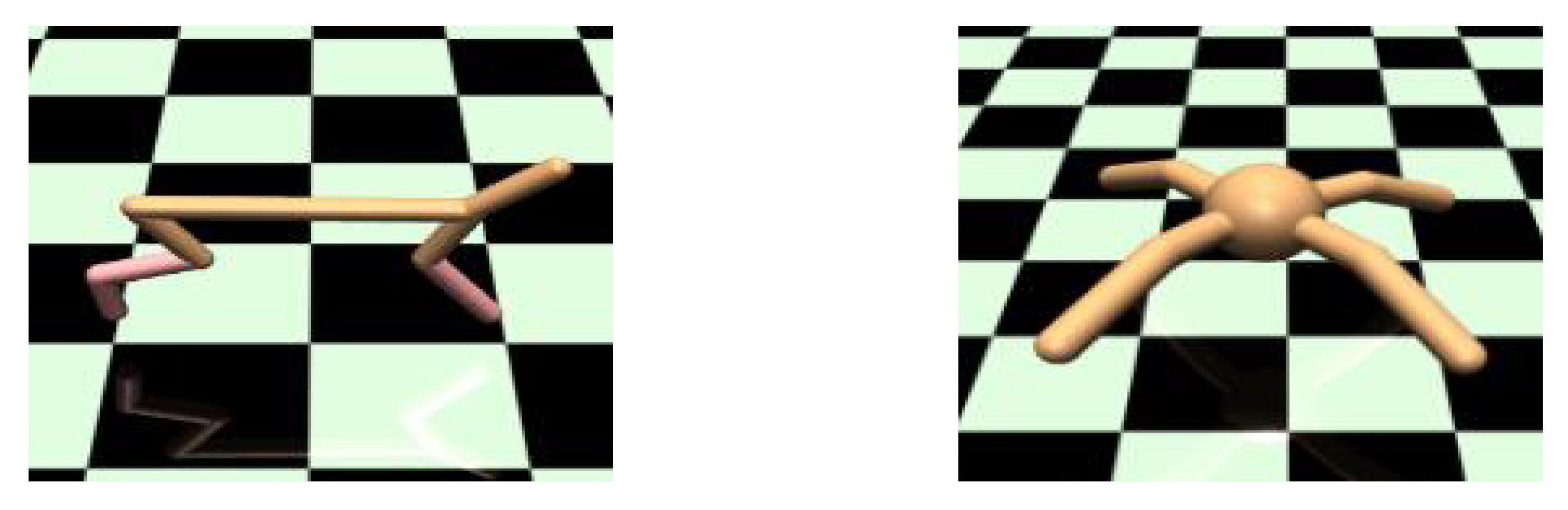
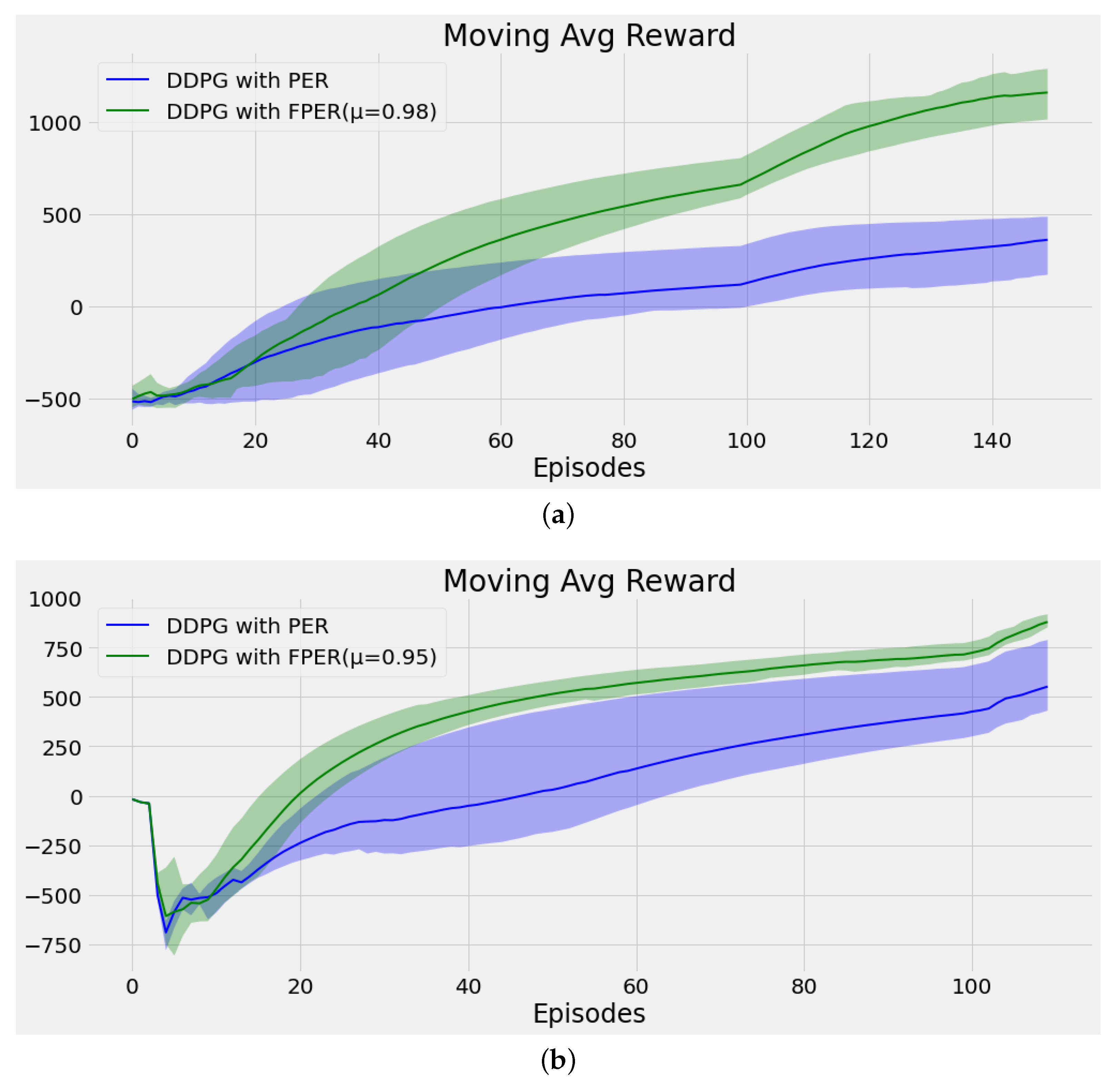
5.3. Continuous Control

Continuous control tasks refer to tasks with continuous action spaces i.e., the number of actions is not defined, but their range can be evaluated. In this paper, two MuJoCo [38] tasks based on OpenAI Gym are used to evaluate the performance of FPER in continuous control tasks: HalfCheetah-v1 and Ant-v1, shown in Figure 5.

Figure 5. From left to right: HalfCheetah-v1, Ant-v1.

DDPG is used in continuous control evaluation. Adam [39] is adopted to train the neural network with a learning rate of $3\times {10}^4$ for the action-value network and actor network. The two networks show similar structure. In our work, there are two hidden layers in both networks and each layer contains 256 hidden units.The discounted factor is set as $0.99$. The buffer size is set as ${10}^4$. The mini-batch size is set as 32, and the updating rate of target network is set as $0.005$. Moreover, the freshness discounted factor for HalfCheetah-v1 is set as $0.98$ and set as $0.95$ for another. A purely exploratory strategy is used for the first 10,000 steps. Gaussian noise $\mathcal{N}(0,0.1)$ is added to each action afterwards.

We compare our Algorithm 2 against DDPG with PER. The lifetime pointer is not combined with FPER in these tasks for reducing surplus computation. Other experimental settings are the same as those in Section 5.1.

Figure 6a compares the plots of FPER and PER, which are applied in HalfCheetah-v1. The learning speed of FPER is obviously faster than PER. The reward of FPER almost increases $100\%$. Figure 6b depicts the curves of FPER and PER in Ant-v1. Although the improvement is not so obvious, FPER still outperforms PER. In a nutshell, the results mean that FPER performs better than PER in continuous control tasks.

Figure 6. Learning curves in continuous control tasks. The shaded region represents the standard deviation of the average evaluation over five trials, and the thick line represents the mean of the average evaluation over five trials. (a) HalfCheetah-v1. (b) Ant-v1.

Table 2 lists the implemented time taken by the agent for different algorithms in different continuous control tasks. Notably, FPER can obtain the same reward in the half of the time steps that PER takes in different environment, demonstrating excellent learning capacity.

Table 2. Implemented time in continuous control tasks.

		Environment	HalfCheetah-v1 $(\mathit{R}\mathit{e}\mathit{w}\mathit{a}\mathit{r}\mathit{d}=500)$	Ant-v1 $(\mathit{R}\mathit{e}\mathit{w}\mathit{a}\mathit{r}\mathit{d}=500)$
	Time Steps
Algorithm
FPER			$7.5\times {10}^4$	$4.5\times {10}^4$
PER			$15\times {10}^4$	$8.5\times {10}^4$

6. Discussion

As known, DRL has achieved impressive results in fields such as robotics. David Silver, a DeepMind researcher in charge of the AlphaGo project, believes “AI = RL + DL”. It is expected that DRL has a huge development scope in the future, and it will profoundly affect people’s real life.

Nowadays, DRL is applied to mostly limited static environments and some deterministic environments. Its application in broad practical scenarios is still difficult due to three main reasons. Firstly, data inefficiency severely limits the application of DRL in practical scenarios. Even some of the best DRL algorithms out there may be impractical due to data inefficiency. Secondly, finding an efficient exploration strategy in continuous high-dimensional action spaces remains challenging. Thirdly, most DRL algorithms are trained with hyper-parameters tuned for a specific task, and these often fail for novel tasks or environments.

We resolved the first aforementioned problem through the presented FPER. To improve data efficiency, it is necessary to collect more data or use the currently available data more effectively. In this paper, FPER can select more valuable data from the replay buffer, resulting in increasing data efficiency. Therefore, FPER can accelerate the convergence speed of DRL algorithms, which makes a great contribution to the convergence of DRL algorithms. Meanwhile, it should be noticed that there are many other factors still limiting the convergence of DRL e.g., inefficient exploration strategy. So, only FPER cannot guarantee the convergence of DRL. Other useful improvement approaches need to be proposed in the future.

In conclusion, FPER can drive to be DRL applied to the real world and will truly change people’s lives.

7. Conclusions

The freshness of experiences implicitly reflects the potential value of experiences. It can improve the performance of PER by adjusting the priority of the experiences based on the freshness accurately.

We successfully run FPER to solve the problem of data efficiency in PER. In FPER, the introduction of a freshness discounted factor $\mu$ properly decreases the priority of experience which has been sampled many times. In this approach, fresh experiences can be replayed more frequently to improve the learning efficiency of DRL algorithms. We validate the effectiveness of FPER in both discrete control tasks and continuous control tasks. The results show that FPER improves both the learning speed and performance of PER in most environments. Furthermore, we propose a lifetime pointer scheme to increase the efficiency of experience replacement and to make the learning process more robust. Our modifications are really simple and can be easily implemented in most algorithms with PER.

Furthermore, the measurement of the experience freshness is not limited. There are lots of priority formulations representing the experiences freshness is negatively correlated with the number of replays. Moreover, other factors may affect the experience freshness. A better approach would theoretically explore more fruitful performance in the future.

References

1. Sutton, R.; Barto, A. Reinforcement Learning: An Introduction; MIT Press: Cambridge, MA, USA, 1998. [Google Scholar]
2. Silver, D.; Huang, A.; Maddison, C.; Guez, A.; Sifre, L.; Driessche, G.V.D.; Schrittwieser, J.; Antonoglou, I.; Panneershelvam, V.; Lanctot, M.; et al. Mastering the Game of Go with Deep Neural Networks and Tree Search. Nature 2016, 529, 484–489. [Google Scholar] [CrossRef] [PubMed]
3. Mnih, V.; Kavukcuoglu, K.; Silver, D.; Rusu, A.; Veness, J.; Bellemare, M.G.; Graves, A.; Riedmiller, M.; Fidjeland, A.K.; Ostrovski, G.; et al. Human-level control through deep reinforcement learning. Nature 2015, 518, 529–533. [Google Scholar] [CrossRef] [PubMed]
4. Kober, J.; Bagnell, J.A.; Peters, J. Reinforcement learning in robotics: A survey. Int. J. Robot. Res. 2013, 32, 1238–1274. [Google Scholar] [CrossRef]
5. Deisenroth, M.P. A Survey on Policy Search for Robotics. Found. Trends Robot. 2011, 2, 1–142. [Google Scholar] [CrossRef]
6. Argall, B.D.; Chernova, S.; Veloso, M.; Browning, B. A survey of robot learning from demonstration. Robot. Auton. Syst. 2009, 57, 469–483. [Google Scholar] [CrossRef]
7. Hu, Y.J.; Lin, S.J. Deep Reinforcement Learning for Optimizing Finance Portfolio Management. In Proceedings of the 2019 Amity International Conference on Artificial Intelligence (AICAI), Dubai, United Arab Emirates, 4–6 February 2019; pp. 14–20. [Google Scholar] [CrossRef]
8. Charpentier, A.; Elie, R.; Remlinger, C. Reinforcement learning in economics and finance. Comput. Econ. 2021, 1–38. [Google Scholar] [CrossRef]
9. Hambly, B.; Xu, R.; Yang, H. Recent advances in reinforcement learning in finance. arXiv 2021, arXiv:2112.04553. [Google Scholar] [CrossRef]
10. Yu, C.; Liu, J.; Nemati, S.; Yin, G. Reinforcement learning in healthcare: A survey. ACM Comput. Surv. (CSUR) 2021, 55, 1–36. [Google Scholar] [CrossRef]
11. Esteva, A.; Robicquet, A.; Ramsundar, B.; Kuleshov, V.; DePristo, M.; Chou, K.; Cui, C.; Corrado, G.; Thrun, S.; Dean, J. A guide to deep learning in healthcare. Nat. Med. 2019, 25, 24–29. [Google Scholar] [CrossRef]
12. Zhang, D.; Han, X.; Deng, C. Review on the research and practice of deep learning and reinforcement learning in smart grids. CSEE J. Power Energy Syst. 2018, 4, 362–370. [Google Scholar] [CrossRef]
13. Mocanu, E.; Mocanu, D.C.; Nguyen, P.H.; Liotta, A.; Webber, M.E.; Gibescu, M.; Slootweg, J.G. On-line building energy optimization using deep reinforcement learning. IEEE Trans. Smart Grid 2018, 10, 3698–3708. [Google Scholar] [CrossRef]
14. Wei, F.; Wan, Z.; He, H. Cyber-attack recovery strategy for smart grid based on deep reinforcement learning. IEEE Trans. Smart Grid 2019, 11, 2476–2486. [Google Scholar] [CrossRef]
15. Tesauro, G. Temporal difference learning and TD-Gammon. Commun. ACM 1995, 38, 58–68. [Google Scholar] [CrossRef]
16. Rummery, G.A.; Niranjan, M. On-Line Q-Learning Using Connectionist Systems; Citeseer: Cambridge, UK, 1994; Volume 37. [Google Scholar]
17. Lin, L.J. Self-Improving Reactive Agents Based on Reinforcement Learning, Planning and Teaching. Mach. Learn. 1992, 8, 293–321. [Google Scholar] [CrossRef]
18. Mnih, V.; Kavukcuoglu, K.; Silver, D.; Graves, A.; Antonoglou, I.; Wierstra, D.; Riedmiller, M. Playing atari with deep reinforcement learning. arXiv 2013, arXiv:1312.5602. [Google Scholar]
19. Hasselt, V.H.; Guez, A.; Silver, D. Deep Reinforcement Learning with Double Q-learning. In Proceedings of the AAAI’16 Proceedings of the Thirtieth AAAI Conference on Artificial Intelligence, Phoenix, AZ, USA, 12–17 February 2016; pp. 2094–2100. [Google Scholar]
20. Wang, Z.; Schaul, T.; Hessel, M.; Hasselt, V.H.; Lanctot, M.; Freitas, D.N. Dueling Network Architectures for Deep Reinforcement Learning. Int. Conf. Mach. Learn. 2016, 32, 1995–2003. [Google Scholar]
21. Hausknecht, M.; Stone, P. Deep recurrent q-learning for partially observable mdps. In Proceedings of the 2015 AAAI Fall Symposium Series, Arlington, VA, USA, 12–14 November 2015. [Google Scholar]
22. Schulman, J.; Levine, S.; Abbeel, P.; Jordan, M.; Moritz, P. Trust region policy optimization. In Proceedings of the International conference on machine learning. PMLR, Lille, France, 6–11 July 2015; pp. 1889–1897. [Google Scholar]
23. Schulman, J.; Wolski, F.; Dhariwal, P.; Radford, A.; Klimov, O. Proximal policy optimization algorithms. arXiv 2017, arXiv:1707.06347. [Google Scholar]
24. Mnih, V.; Badia, A.P.; Mirza, M.; Graves, A.; Lillicrap, T.; Harley, T.; Silver, D.; Kavukcuoglu, K. Asynchronous methods for deep reinforcement learning. In Proceedings of the International Conference on Machine Learning, PMLR, New York, NY, USA, 19–24 June 2016; pp. 1928–1937. [Google Scholar]
25. Lillicrap, T.; Hunt, J.; Pritzel, A.; Heess, N.; Erez, T.; Tassa, Y.; Silver, D. Continuous control with deep reinforcement learning. arXiv 2015, arXiv:1509.02971. [Google Scholar]
26. Fujimoto, S.; Hoof, H.V.; Meger, D. Addressing Function Approximation Error in Actor-Critic Methods. arXiv 2018, arXiv:1802.09477. [Google Scholar]
27. Bellemare, M.G.; Dabney, W.; Munos, R. A distributional perspective on reinforcement learning. In Proceedings of the International Conference on Machine Learning, PMLR, Sydney, Australia, 6–11 August 2017; pp. 449–458. [Google Scholar]
28. Dabney, W.; Rowland, M.; Bellemare, M.; Munos, R. Distributional reinforcement learning with quantile regression. In Proceedings of the AAAI Conference on Artificial Intelligence, New Orleans, LA, USA, 2–3 February 2018; Volume 32. [Google Scholar]
29. Schaul, T.; Quan, J.; Antonoglou, I.; Silver, D. Prioritized Experience Replay. arXiv 2015, arXiv:1511.05952. [Google Scholar]
30. Zhang, S.; Sutton, R.S. A Deeper Look at Experience Replay. arXiv 2017, arXiv:1712.01275. [Google Scholar]
31. Liu, R.; Zou, J. The Effects of Memory Replay in Reinforcement Learning. In Proceedings of the 56th Allerton Conference on Communication, Control, and Computing, Monticello, IL, USA, 2–5 October 2018. [Google Scholar]
32. Hou, Y.; Liu, L.; Wei, Q.; Xu, X.; Chen, C. A novel DDPG method with prioritized experience replay. In Proceedings of the IEEE International Conference on Systems, Banff, AB, Canada, 5–8 October 2017. [Google Scholar]
33. Shen, K.H.; Tsai, P.Y. Memory Reduction through Experience Classification f or Deep Reinforcement Learning with Prioritized Experience Replay. In Proceedings of the 2019 IEEE International Workshop on Signal Processing Systems (SiPS), Nanjing, China, 20–23 October 2019. [Google Scholar]
34. Bellman, R. Dynamic programming. Science 1966, 153, 34–37. [Google Scholar] [CrossRef] [PubMed]
35. Zhu, J.; Wu, F.; Zhao, J. An Overview of the Action Space for Deep Reinforcement Learning. In Proceedings of the 2021 4th International Conference on Algorithms, Computing and Artificial Intelligence, Sanya, China, 22–24 December 2021; pp. 1–10. [Google Scholar]
36. Brockman, G.; Cheung, V.; Pettersson, L.; Schneider, J.; Schulman, J.; Tang, J.; Zaremba, W. OpenAI Gym. arXiv 2016, arXiv:1606.01540. [Google Scholar]
37. Tieleman, T.; Hinton, G. Lecture 6.5-rmsprop: Divide the gradient by a running average of its recent magnitude. COURSERA Neural Netw. Mach. Learn. 2012, 4, 26–31. [Google Scholar]
38. Todorov, E.; Erez, T.; Tassa, Y. MuJoCo: A physics engine for model-based control. In Proceedings of the 2012 IEEE/RSJ International Conference on Intelligent Robots and Systems, Vilamoura-Algarve, Portugal, 7–12 October 2012. [Google Scholar]
39. Kingma, D.; Ba, J. Adam: A Method for Stochastic Optimization. arXiv 2014, arXiv:1412.6980. [Google Scholar]
Publisher’s Note: MDPI stays neutral with regard to jurisdictional claims in published maps and institutional affiliations.
Article Metrics
Citations
Article Access Statistics
Multiple requests from the same IP address are counted as one view.