A Scaling Transition Method from SGDM to SGD with 2ExpLR Strategy

Abstract

In deep learning, the vanilla stochastic gradient descent (SGD) and SGD with heavy-ball momentum (SGDM) methods have a wide range of applications due to their simplicity and great generalization. This paper uses an exponential scaling method to realize a smooth and stable transition from SGDM to SGD, which combines the advantages of the fast training speed of SGDM and the accurate convergence of SGD (named TSGD). We also provide some theoretical results on the convergence of this algorithm. At the same time, we take advantage of the learning rate warmup strategy’s stability and the learning rate decay strategy’s high accuracy. A warmup–decay learning rate strategy with double exponential functions is proposed (named 2ExpLR). The experimental results on different datasets for the proposed algorithms indicate that the accuracy is improved significantly and that the training is faster and more stable.

1. Introduction

In recent years, with the development of deep-learning technologies, many neural network models have been proposed, such as FCNN [1], LeNet [2], LSTM [3], ResNet [4], DensNet [5], and so on. They also have an extensive range of applications [6,7,8]. Most networks, such as CNN and RNN, are supervised types of deep learning that require a training set to teach models to yield the desired output. Gradient Descent (GD) is the most common optimization algorithm in machine learning and deep learning, and it plays a significant role in training.

In practical applications, the SGD (a type of GD algorithm) is one of the most dominant algorithms because of its simplicity and low computational complexity. However, one disadvantage of SGD is that it updates parameters only with the current gradient, which leads to slow speeds and unstable training. Researchers have proposed new variant algorithms to address these deficiencies.

Polyak et al. [9] proposed a heavy-ball momentum method and used the exponential moving average (EMA) [10] to accumulate the gradient to speed up the training. Nesterov accelerated gradient (NAG) [11] is a modification of the momentum-based update, which uses a look-ahead step to improve the momentum term [12]. Subsequently, researchers improved the SGDM and proposed synthesized Nesterov variants [13], PID control [14], AccSGD [15], SGDP [16], and so on.

A series of adaptive gradient descent methods and their variants have also been proposed. These methods scale the gradient by some form of past squared gradients, making the learning rate automatically adapt to changes in the gradient, which can achieve a rapid training speed with an element-wise scaling term on learning rates [17].

Many algorithms produce excellent results, such as AdaGrad [18], Adam [19], and AMSGrad [20]. In neural-network training, these methods are more stable, faster, and perform well on noisy and sparse gradients. Although they have made significant progress, the generalization of adaptive gradient descent is often not as good as SGD [21]. There are some additional issues [22,23].

First, the solution of adaptive gradient methods with second moments may fall into a local minimum of poor generalization and even diverge in certain cases. Then, the practical learning rates of weight vectors tend to decrease during training, which leads to sharp local minima that do not generalize well. Therefore, some trade-off methods of transforming Adam to SGD are proposed to obtain the advantages of both, such as Adam-Clip (p, q) [24], AdaBound [25], AdaDB [26], GWDC [27], linear scaling AdaBound [28], and DSTAdam [29]. Can we transfer this idea to SGDM and SGD?

This study is strongly motivated by recent research on the combination of SGD and SGDM under the QHM algorithm [30]. They gave a straightforward alteration of momentum SGD, averaging a vanilla SGD step and a momentum step, and obtained good results in experiments. It can be explained as a $v-$ weighted average of the momentum update step and the vanilla SGD update step, and the authors provided a recommended rule of thumb $v=0.7$. However, in many scenarios, it is not easy to find the optimal value of v. On this basis, we conducted a more in-depth study on the combination of SGDM and SGD.

In this paper, first, we analyze the disadvantages of SGDM and SGD and propose a scaling method to achieve a smooth and stable transition from SGDM to SGD, combining the fast training speed of the SGDM and the high accuracy of the SGD. At the same time, we combine the advantages of the warmup and decay strategy and propose a warmup–decay learning rate strategy with double exponential functions. This makes the training algorithm more stable in the early stage and more accurate in the later stage. The experimental results show that our proposed algorithms had a faster training speed and better accuracy in the neural network model.

2. Preliminaries

Optimization problem. $f:$ ${\mathbb{R}}^n\to \mathbb{R}$ is the objective function, and $f\left(\theta ,\zeta \right)\in C^1$ is continuously differentiable, where $\theta$ is the optimized parameter. Considering the following convex optimization problem [31]:

$$\underset{\theta \in R^n}{min}f(\theta ,\zeta ),$$

(1)

where $\zeta$ is a stochastic variable. Applying the gradient descent method to solve the above minimization problem:

$${\theta }_{t+1}={\theta }_t-\eta g_t,$$

(2)

where $\eta$ is the constant step size, $g_t$ is the descent direction, and $\theta$ is the parameter that needs to be updated.

SGD. SGD uses the current gradient of the loss function to update the parameters [32]:

$$g_t\leftarrow \nabla f\left(\theta ,\zeta \right),$$

(3)

where f is the loss function and $\nabla f\left(\theta ,\zeta \right)$ is the gradient of the loss function.

SGDM. The momentum method considers the past gradient information and uses it to correct the direction, which speeds up the training. The update rule of the heavy-ball momentum method [33] is

$$\begin{array}{c}{m}_t=\beta m_{t-1}+\left(1-\beta \right)\nabla f\left(\theta ,\zeta \right)\hfill \\ g_t\leftarrow m_t,\hfill \end{array}$$

(4)

where $m_t$ is the momentum and $\beta$ is the momentum factor.

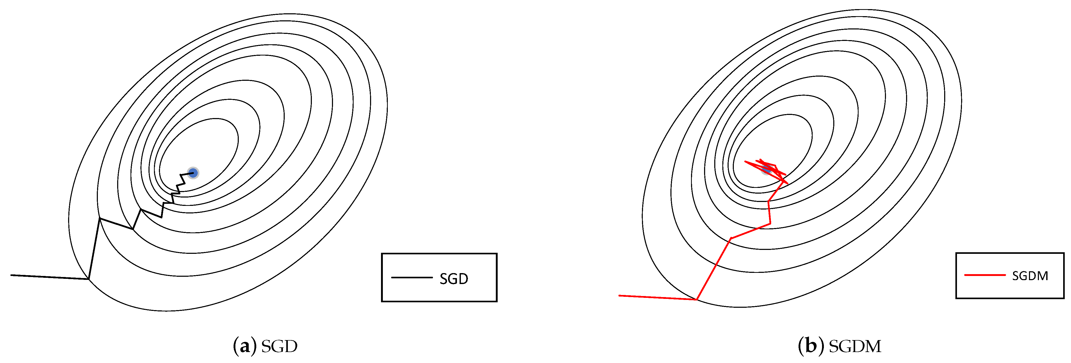
Efficiency of SGD and SGDM. In convex optimization, the gradient descent method can search the optimal global solution of the objective function by the steepest descent. However, it has a series of zigzag paths in the iteration process, which seriously affects the training speed. We can explore the root of this defect using theoretical analysis. Using exact line search to solve the convex optimization problems (1):

$$\begin{array}{c}\phi \left(\lambda \right)=f\left({\theta }^{\left(t\right)}+\lambda d^{\left(t\right)},\zeta \right)\hfill \\ d^{\left(t\right)}=-\nabla f\left({\theta }^{\left(t\right)},\zeta \right).\hfill \end{array}$$

(5)

In order to find the minimum point along the direction $d^{\left(t\right)}$ from $x^{\left(t\right)}$, let

$${\phi }^{\prime }\left(\lambda \right)=\nabla f{\left({\theta }^{\left(t\right)}+{\lambda }_t{d}^{\left(t\right)},\zeta \right)}^T{d}^{\left(t\right)}=0.$$

(6)

Thus,

$$-\nabla f{\left({\theta }^{\left(t+1\right)},\zeta \right)}^T\nabla f\left({\theta }^{\left(t\right)},\zeta \right)=0.$$

(7)

We know that $d^{\left(t+1\right)}=-\nabla f\left({\theta }^{\left(t+1\right)},\zeta \right)$ and $d^{\left(t\right)}=-\nabla f\left({\theta }^{\left(t\right)},\zeta \right)$ are orthogonal. This shows that the path of the iterative sequence {$f\left({\theta }^t,\zeta \right)$} is a zigzag. When it is close to the minimum point, the step size of each movement will be tiny and seriously affects the speed of convergence as shown in Figure 1a.

Polyak et al. [9] proposed SGD with a heavy-ball momentum algorithm to mitigate the zigzag oscillation and accelerate training. The update direction of the SGDM is the EMA [10] of the current gradient and the past gradient to speed up the training speed and reduce the vibration in SGD. The momentum of the SGDM is

$$m_t=\sum _{i=1}^t\left(1-\beta \right){\beta }^{t-i}{g}_i.$$

(8)

However, in the later stage of training, there is a defect in using EMA for the gradient. The accumulation of gradients may lead to a faster speed of momentum and not stop in time when it is close to the optimum. This may oscillate in a region around the optimal solution ${\theta }^{*}$ and cannot stably converge as shown in Figure 1b. At the same time, the gradients that are too far may have little helpful information, and the momentum can be calculated using the gradients of the last n times, such as AdaShift [34]. The negative gradient direction of the loss function is the optimal direction for the current parameter updating. The updating direction is no longer the fastest descent direction when using momentum. When it is close to the optimal solution, the stochastic gradient descent method is more accurate and is more likely to find the optimal point.

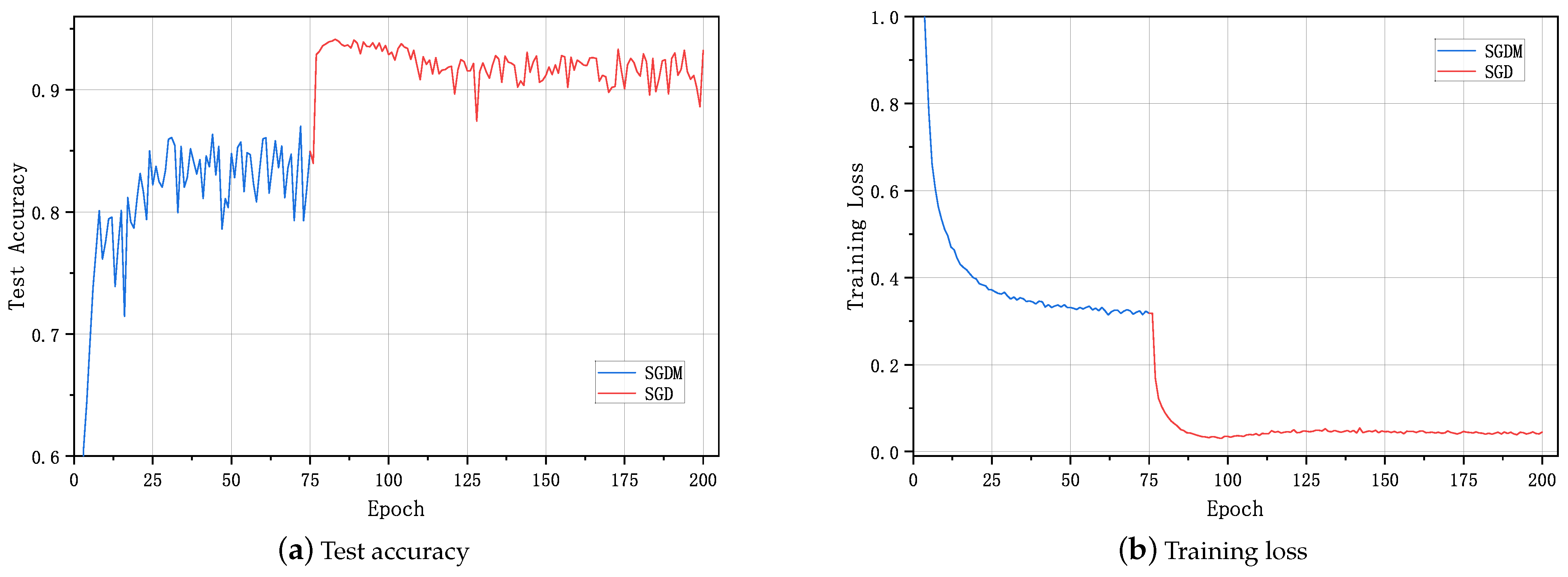
For more information, we use the ResNet18 to train the CIFAR10 dataset, and the first 75 epochs use the SGDM algorithm (hyperparameter setting: weight_decay = 5 × 10${}^{-3}$, $lr$ = $0.1$, $\beta$ = $0.9$). After the 75-th epoch, we only change the updating direction from momentum to gradient (descent direction if epoch < 76: $m_t$ else: $g_t$, no other setting is changed). Figure 2a shows the accuracy curve of the test set during the training. It can be seen that, after the accuracy increases rapidly from starting and then enters the plateau after about the 25-th epochs, the accuracy no longer increases.

After the 75-th epoch, the current gradient is used to update the parameters, showing that the accuracy significantly improved. Figure 2b records the training loss. It can be seen that the loss of the SGD is faster and smaller. If we combine the advantages of SGDM and SGD in this way, the training algorithm can have both the fast training speed of SGDM and the high accuracy of SGD.

3. TSGD Algorithm

Based on the above analysis and the basis of the QHM algorithm, we provide a middle ground that combines preferable features from both. This includes the advantages of SGDM with a fast training speed and of SGD with high accuracy. A scaling transition method from SGDM to SGD is proposed—named TSGD. A scaling function ${\rho }^t$ is introduced to gradually scale the momentum direction to the gradient direction as the iteration, which achieves a smooth and stable transition from SGDM to SGD. The specific algorithm is represented in Algorithm 1.

Algorithm 1: A Scaling Transition method from SGDM to SGD (TSGD)

Input: initial parameters: ${\theta }_1\in \mathcal{F}$, $\eta$, $\beta$, $\rho$.

Initialize: $m_0=0.$

1: for$t=1$ to T do

2:    $g_t=\nabla f_t\left({\theta }_t\right)$

3:    $m_t=\beta m_{t-1}+\left(1-\beta \right)g_t$

4:    ${\widehat{m}}_t=\left(m_t-g_t\right){\rho }^t+g_t$

5:    ${\theta }_{t+1}={\theta }_t-\eta {\widehat{m}}_t$

6: end for

In Algorithm 1, $g_t$ is the gradient of loss function, f in the t-th iteration, and $m_t$ is the momentum. ${\widehat{m}}_t$ is the scaled momentum, ${\theta }_t$ is the optimized parameter, ${\rho }^t$ is the scaling function, and ${\rho }^t\in \left[0,1\right]$. We provide recommended rules of the hyperparameters $\rho$ and $\beta$, which are ${\rho }^T=0.01$ and $\beta =0.9$, where T is the number of iterations, $T=ceil(samplesize/batchsize)\ast epochs$.

Gitman et al. [35] made a detailed convergence analysis on the general form of the QHM algorithm. The TSGD algorithm proposed in this section conforms to the general form of the QHM algorithm. Therefore, the TSGD algorithm has the same convergence conclusion as the general form of the QHM algorithm. Theorem 1 gives the convergence theory of the TSGD algorithm based on the literature [35].

Theorem 1.

Let f satisfy the condition in the literature [35]. Additionally, assume that $0\le {\rho }^t\le 1$ and the sequences $\left\{{\eta }_t\right\}$ and $\left\{{\beta }_t\right\}$ satisfy the following conditions:

$$\sum _{t=0}^{\infty }{\eta }_t=\infty ,\sum _{t=0}^{\infty }{\eta }_t^2=\infty ,\underset{t\to \infty }{lim}{\beta }_t=0,\overline{\beta }\stackrel{\Delta }{=}\underset{t}{sup}{\beta }_t<1.$$

Then, the sequence $\left\{{\theta }_t\right\}$ that is generated by the TSGD Algorithm 1 satisfies:

$$\underset{t\to \infty }{lim}∥\nabla f\left({\theta }_t\right)∥=0.$$

Moreover, we have:

$$\underset{t\to \infty }{lim}supf\left({\theta }_t\right)=\underset{t\to \infty ,∥\nabla f\left({\theta }_t\right)∥\to 0}{limsup}f\left({\theta }_t\right).$$

Theorem 1 implies that TSGD can converge, which is similar to SGD-type optimizers. Through exponential decay in step 4 of the TSGD Algorithm, the updated direction smoothly and stably transforms the momentum direction of SGDM to the gradient direction of SGD as iterations. In the early stage of training, the number of iterations is small, ${\rho }^t$ is close to 1, and the updated direction is

$${\widehat{m}}_t\leftarrow m_t,$$

which can speed up the training speed. In the later stage, with the increase of iterations, the number of iterations is large, and ${\rho }^t$ is close to 0. The updated direction is gradually transformed to

$${\widehat{m}}_t\leftarrow g_t.$$

When the iterative sequence closes to the optimal solution, gradient direction is used to update the parameters and is more accurate. Thus, TSGD has the advantages of both faster speed of SGDM and high accuracy of SGD. TSGD does not need to calculate the second moment of the gradient, which saves computational resources compared to the adaptive gradient descent method.

4. The Warmup Decay Learning Rate Strategy with Double Exponential Functions

The learning rate (LR) is a crucial hyperparameter to tune for practical training of deep neural networks and controls the rate or speed at which the model learns each iteration [36]. If the learning rate is too large, this may cause oscillation and divergence. On the contrary, training may progress slowly and even stop if the rate is too small. Thus, many learning rate strategies have been proposed and appear to work well, such as warmup [4], decay [37], restart techniques [38], and cyclic learning rates [39]. In this section, we mainly focus on the warmup and decay strategies.

On the one hand, the idea of warmup was proposed in ResNet [4]. They used 0.01 to warm up the training until the training error was below 80% (about 400 iterations) and then went back to 0.1 and continued training. In the early stage of training, due to many random parameters in the model, if a large learning rate is used, the model may be unstable and fall into a local optimum, which is challenging to fix. Therefore, we use a small learning rate to make the model learn certain prior knowledge and then use a large learning rate for training when the model is more stable. It can use less aggressive learning rates at the start of training [40]. Implementations of the warmup strategy include constant warmup [4], linear warmup [41], and gradual warmup [40].

On the other hand, decay is also a popular strategy in neural-network training. The decay can speed up the training using a larger learning rate at the beginning and can converge stably using a smaller learning rate after. Not only does this show good results [24,25,34,42] in practical applications but also the learning rate is required to decay in the theoretical convergence analysis, such as ${\eta }_t=1/t$ [43], ${\eta }_t=1/\sqrt{t}$ [42]. The specific implementation of learning rate decay is as follows: step decay [26], linear attenuation [44], exponential decay [45], etc.

To ensure better performance of the training algorithm, we combined the warmup and decay strategies. The warmup strategy was used for a small number of iterations in the early stage of training, and then the decay strategy was used to decrease the learning rate gradually. In this way, the model can learn stably early on, train fast in the middle, and converge accurately later.

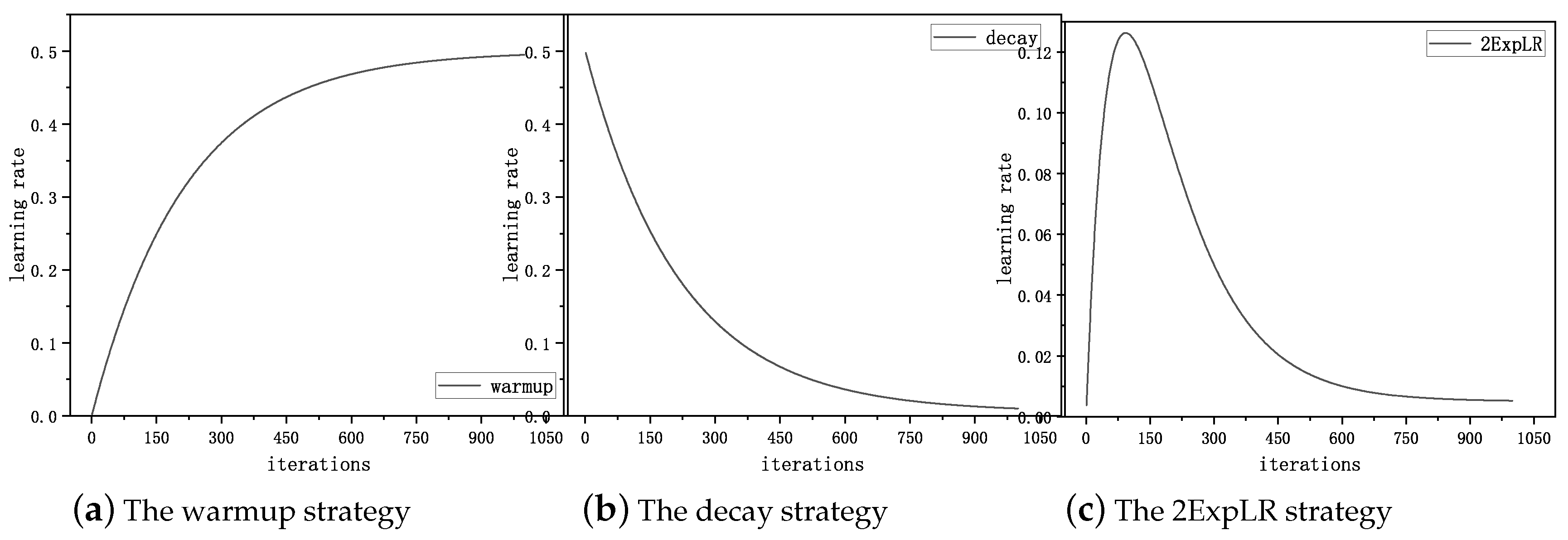
First, an exponential function is used in the warmup stage to gradually increase the learning rate from zero to the upper learning rate as shown in Figure 3a. The numerical formula is as follows

$$l{r}_{warmup}=l{r}_u\left(1-{\rho }_1^t\right).$$

(9)

Second, an exponential function is also used in the decay stage to gradually decrease the learning rate from the upper learning rate to the lower learning rate as shown in Figure 3b. The numerical formula is as follows

$$l{r}_{decay}=\left(l{r}_u-l{r}_l\right){\rho }_2^t+l{r}_l.$$

(10)

The main idea of the warmup–decay learning rate strategy is that the learning rate can increase in the warmup stage and decrease in the decay stage. Therefore, we combine the above two processes, and the warmup–decay learning rate strategy with double exponential functions (2ExpLR) is proposed as shown in Figure 3c. The numerical formula is as follows

$$l{r}_{w-d}=\left(\left(l{r}_u-l{r}_l\right){\rho }_1^t+l{r}_l\right)\left(1-{\rho }_2^t\right).$$

(11)

Similarly, we also provide recommended rules of the hyperparameters ${\rho }_1,{\rho }_2$ as with $\rho$, that are ${\rho }_1^T={\rho }_2^T=l{r}_l\ast {10}^{-1}$. Thus, ${\rho }_1,{\rho }_2$ can be easily calculated using ${\rho }_1={\rho }_2={10}^{\left(lgl{r}_l-1\right)/T}$.

In Figure 3, we know that 2ExpLR does not need to set the transition point from warmup to decay manually, compared with other strategies [24,25,26]. At the same time, we achieve a smooth and stable transition from warmup to decay through 2ExpLR. This gives the training algorithm a faster convergence speed and higher accuracy.

The TSGD algorithm with the 2ExpLR strategy is described as Algorithm 2.

Algorithm 2: Scaling Transition from SGDM to SGD with 2Exp learning rate (TSGD+2ExpLR)

Input: initial parameters: ${\theta }_1\in \mathcal{F}$, $l{r}_l$, $l{r}_u$, $\rho$, ${\rho }_1$, ${\rho }_2$, $\beta$, ${\eta }_t$.

Initialize: $m_0=0$

1: for $t=1$ to T do

2:    $g_t=\nabla f_t\left({\theta }_t\right)$

3:    $m_t=\beta m_{t-1}+\left(1-\beta \right)g_t$

4:    ${\widehat{m}}_t=\left(m_t-g_t\right){\rho }^t+g_t$

5:    ${\eta }_t=\left(\left(l{r}_u-l{r}_l\right){\rho }_1^t+l{r}_l\right)\left(1-{\rho }_2^t\right)$

6:    ${\theta }_{t+1}={\theta }_t-{\eta }_t{\widehat{m}}_t$

7: end for

5. Extension

The scaling transition method on the gradient can be extended to other applications. We can abstract this scaling transition process providing a general framework for the parameter transition from one state to another.

For example, neural networks have been widely used in many fields to solve problems. During the training process, the input data type and amount directly influence the performance of the ANN model [46]. If the data is dirty, contains large amounts of noise, the data size is too small, or the training time is too long, etc., the model can be affected by overfitting [47]. Various regularization techniques have been proposed and developed for neural networks to solve these problems. The regularization technique is used to avoid overfitting of the network and has more parameters than the input data and is used for a network learned with noisy inputs [48], such as L1 and L2 regularization methods.

The model has not learned any knowledge in the early stage of training, and using regularization at this time may result in harmful effects on the model. Therefore, we can train the model generally at the beginning and then use the regularization strategy to train the model in the later stage. Thus, we can implement the scaling transition framework as follows

$$\theta =arg\underset{\theta }{min}\frac{1}{N}\sum _{i=1}^N\left(L\left({\widehat{y}}_i,y_i\right)+\left(\left(0-\lambda R\left(\theta \right)\right){\rho }^t+\lambda R\left(\theta \right)\right)\right),$$

(12)

where $L(\ast )$ is the loss function, N is the number of samples, ${\widehat{y}}_i$ is the predicted value, and $y_i$ is the actual value. $\lambda$ is a non-negative regularization parameter, $R(\ast )$ is a regularization function, such as $L_2={∥\theta ∥}_2^2$, or $L_1={∥\theta ∥}_1$.

6. Experiments

In this section, to verify the performance of the proposed TSGD and TSGD+2ExpLR, we compared them with other algorithms, including SGDM and Adam. Specifically, we used IRIS, CASIA-FaceV5, and CIFAR classification tasks in the experiments. We set the same random seed through PyTorch to ensure fairness. The architecture we chose for the experiments was ResNet-18. The computational setup is shown in

Table 1. The computational setup.

OS	CentOS 8.3	Dataset storage location	OS File system
Processor-CPU	Intel Core i7-6500U	CPU-Memory	$32.0\mathrm{GB}$
Processor-GPU	Quadro P600	GPU-Memory	$2.0\mathrm{GB}$
Programming language	Python $\mathrm{3.7.10}$	Development framework	Pytorch $\mathrm{1.7.0}$

. Our implementation is available at https://github.com/kunzeng/TSGD (accessed on 20 November 2022).

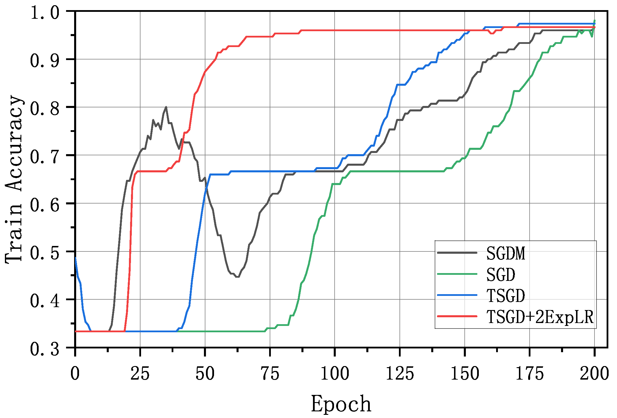
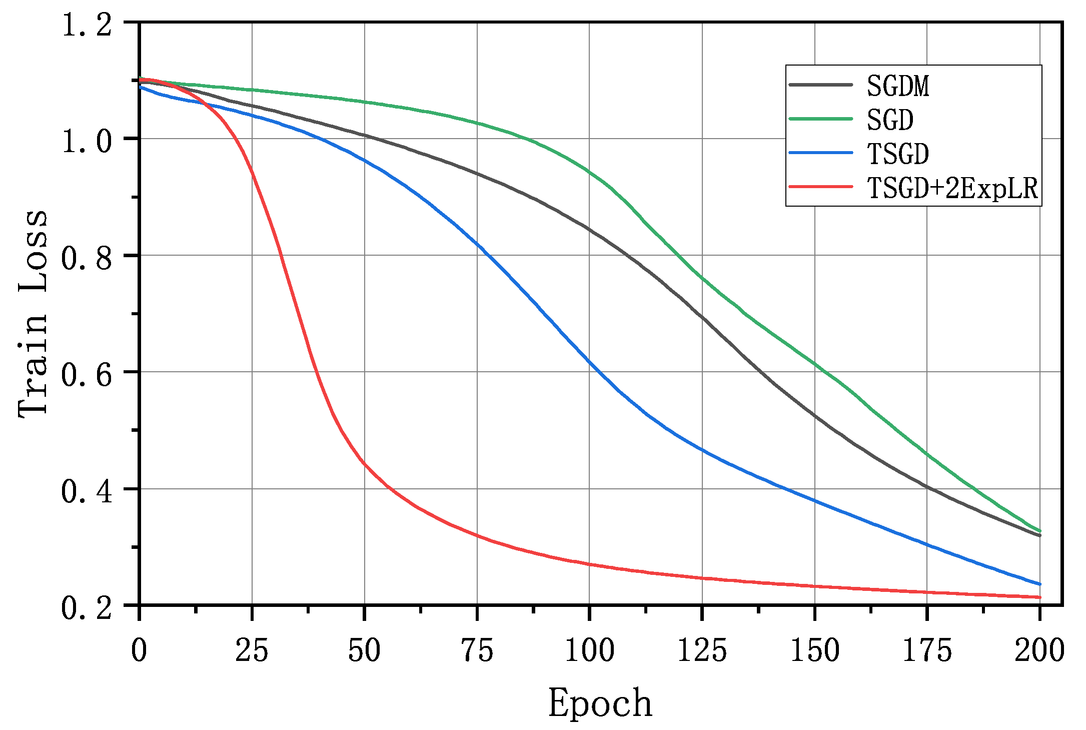
IRIS and BP neural network. The IRIS dataset is a classic dataset for classification, machine learning, and data visualization. This dataset includes three iris species with 50 samples of each and some properties of each flower. An excellent way to determine the correct learning rates is to perform experiments using a small but representative sample of the training set, and the IRIS dataset is a good fit. Due to the small number of samples, we used all 150 samples as the training set. The performance of each algorithm is represented by the accuracy and loss value on the training set. We set the relevant parameters using empirical values and a grid search: samplesize = 150, epoch = 200, batchsize = 1, lr(SGD: 0.003, SGDM: 0.05, TSGD: 0.03), up_lr = 0.5, low_lr = 0.005, rho = 0.977237, and rho1 = rho2 = 0.962708. The experimental results show that the method achieves its expected effect. In Figure 4 and Figure 5, the training process of SGDM has more oscillations, and the convergence speed of SGD is slower. However, TSGD is more stable and faster than SGDM and SGD. It is astonishing that the TSGD+2ExpLR algorithm is stable during training and increases accuracy quickly.

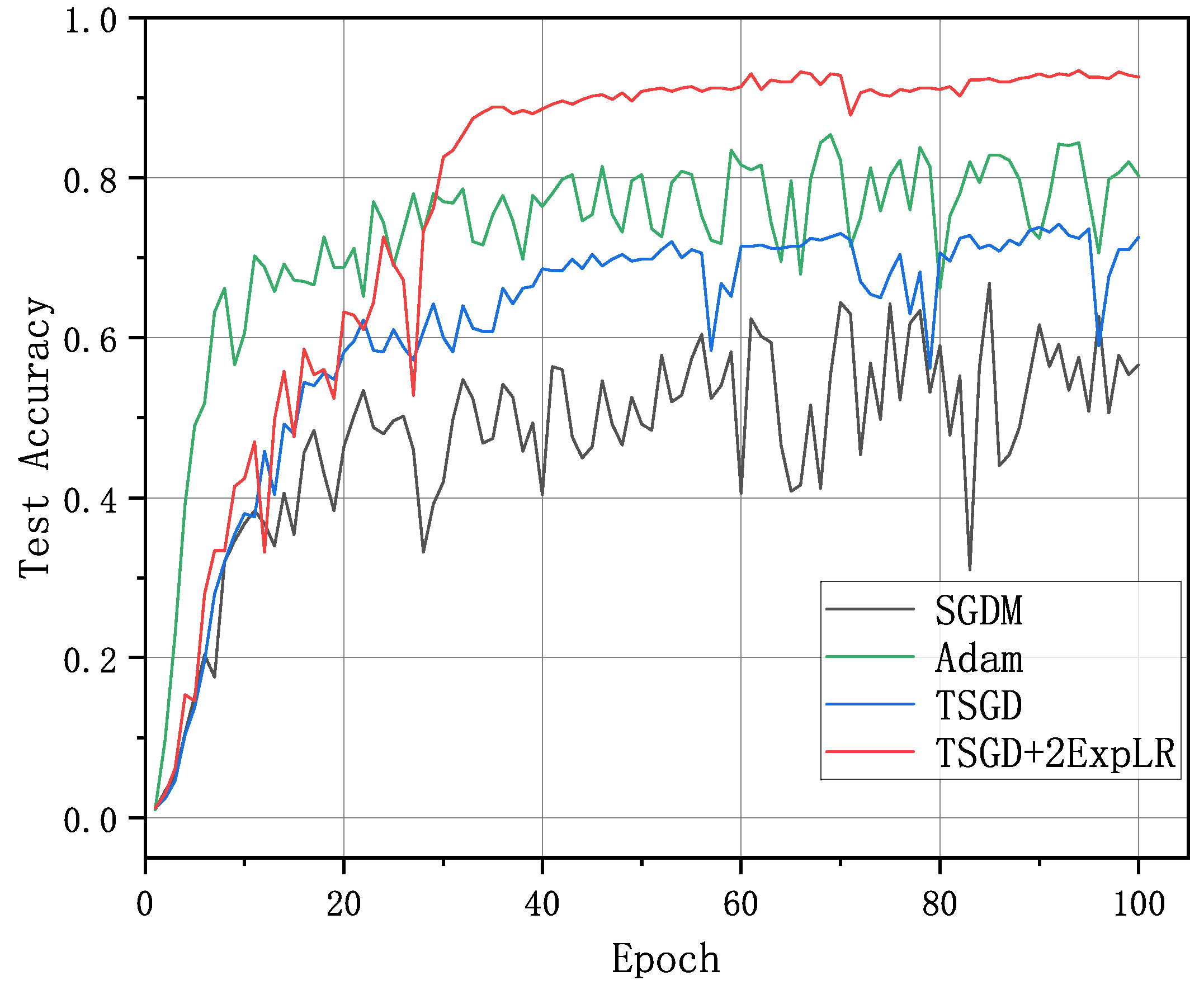
CASIA-FaceV5 and ResNet18. The CASIA-FaceV5 contains 2500 color facial images of 500 subjects. All face images are 16-bit color BMP files, and the image resolution is 640∗480. Typical intra-class variations include the illumination, pose, expression, and eye-glasses imaging distance, which provides a remarkable ability to distinguish between different algorithms. We preprocessed it for better training and reshaped it to 100 × 100. The parameters were set as: samplesize = 2500, epoch = 100, batchsize = 10, lr = 0.1, $l{r}_u$ = 0.5, $l{r}_l$ = 0.005, then T = ceil(samplesize/batchsize) ∗ epoch = 25,000, and thus $\rho$ = ${10}^{\left(log\left({\rho }^T,10\right)/T\right)}\approx 0.999815.$ This is also applicable to ${\rho }_1={\rho }_2=0.999696.$ The experimental results are in Figure 6 and Figure 7. Although we can observe that the accuracy of the TSGD algorithm does not exceed 1 Adam, it exceeds the SGD algorithm, and the training process is more stable. The main reason may be that the CASIA-FaceV5 dataset has fewer samples and more categories, and each category has only five samples. The Adam algorithm is more suitable for this scenario. The accuracy of the TSGD+2ExpLR algorithm is much higher than that of other algorithms. The loss value is also much lower than other algorithms, and the training process is more stable.

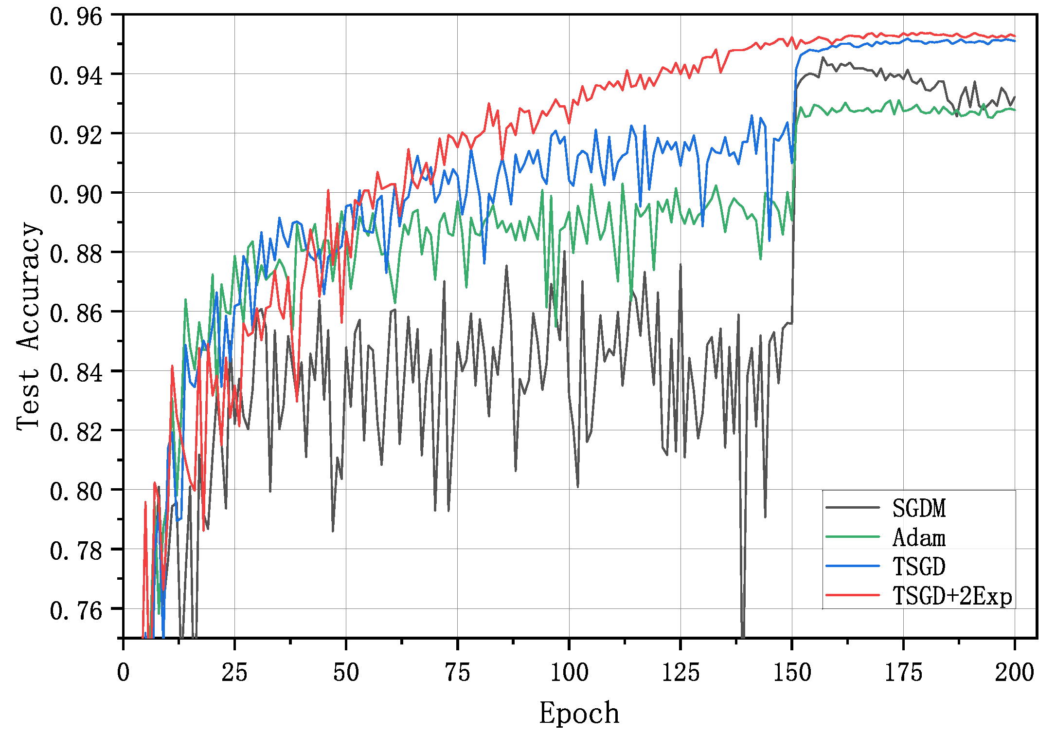
Cifar10 and ResNet18. The CIFAR10 dataset was collected by Hinton et al. [49]. It contains 60,000 color images in 10 categories, with a training set of 50,000 images and a test set of 10,000 images. The parameters are adjusted: epoch = 200, batchsize = 128, $\rho =0.9999411$, ${\rho }_1={\rho }_2=0.9999028$, $lr$ = 0.1, $l{r}_u$ = 0.5, and $l{r}_l$ = 0.005. The other parameters were the same as the above or were the default values recommended by the model. The architecture we used was ResNet18, and the learning rate was divided by 10 at epoch 150 for SGDM, Adam, and TSGD.

Figure 8 shows the test accuracy curves of each optimization method. As we can see, SGDM had the lowest accuracy and more oscillation before 150 epochs, and Adam had a fast speed but lower accuracy after 150 epochs. It is evident that the TSGD and TSGD+2ExpLR had higher accuracy, and the accuracy curves were smoother and more stable. The speed of TSGD even exceeded the speed of Adam.

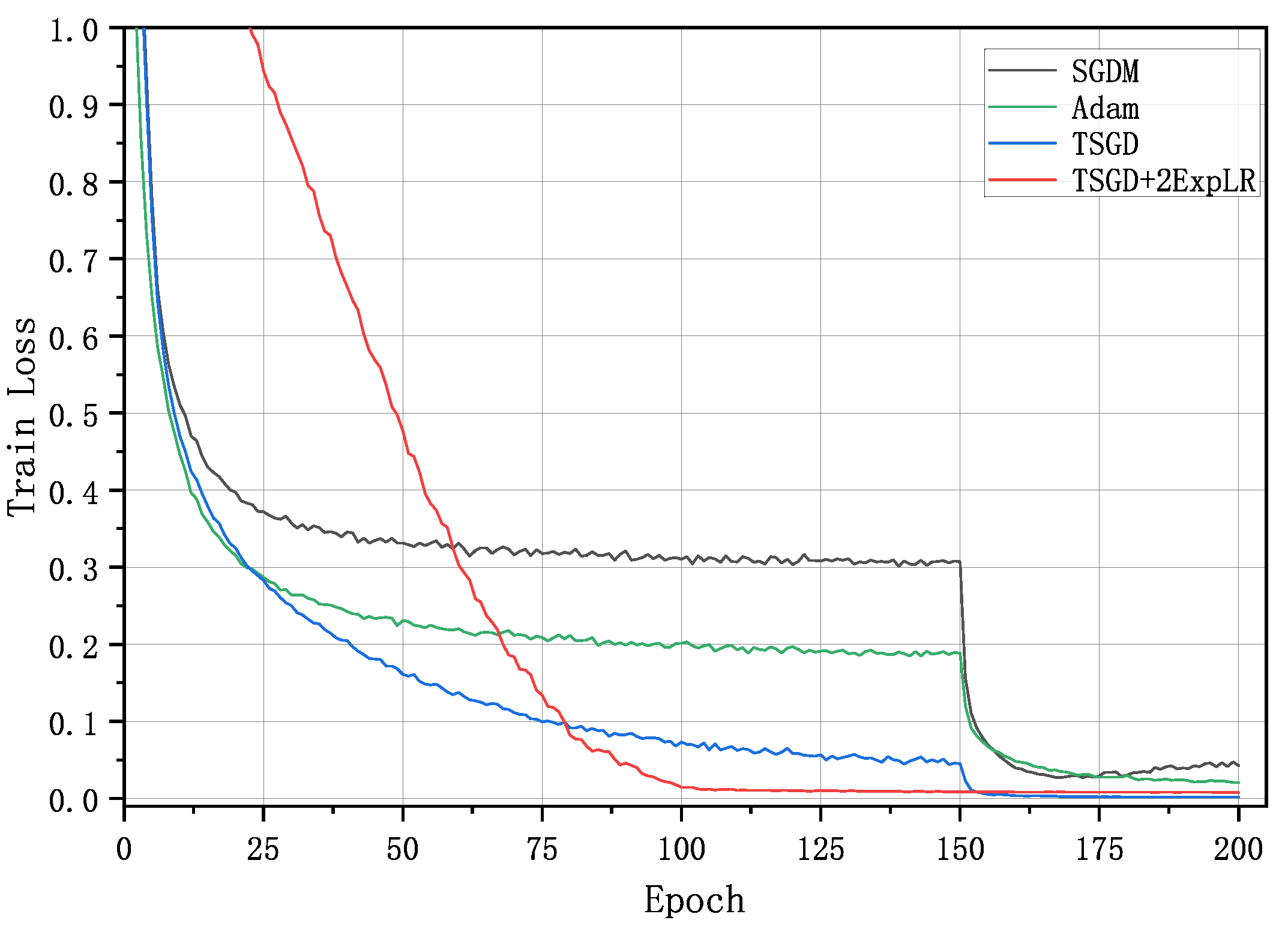
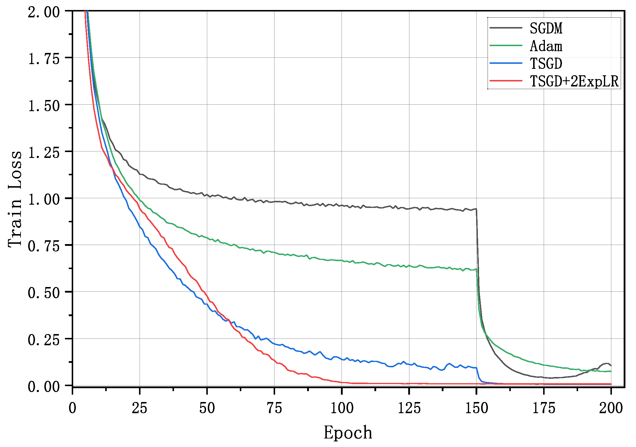
Figure 9 shows the loss of different algorithms on the training set. At the beginning of training, the loss of TSGD decreases slowly, possibly due to the small learning rate of the warmup stage to make the model stable. However, it can be seen that the loss of the TSGD algorithm decreases faster, and the loss is the smallest in the later stage.

Cifar100 and ResNet18. We also present our results for CIFAR100. The task is similar to Cifar10; however, Cifar100 has 10 categories, and each category has 10 subcategories for a total of 100 categories. The parameters are the same as CIFAR10. We show the performance curves in Figure 10 and Figure 11. It can be seen that the performances of each algorithm on CIFAR100 are similar to those of CIFAR10. The two algorithms proposed in this paper can hold the top two spots in all, and the curves are still smoother and more stable. In particular, in TSGD+2ExpLR, the accuracy reaches its peak at about 100 epochs, which reflects the effect of the warmup–decay learning rate strategy with double exponential functions. The loss of the TSGD and TSGD+2ExpLR algorithms decreases faster and finally has a minor loss, almost close to zero. The TSGD and TSGD+2ExpLR are considerably improved over SGDM and Adam, with faster speed and higher accuracy.

7. Conclusions

In this paper, we combined the advantages of SGDM with a fast training speed and SGD with high accuracy and proposed a scaling transition method from SGDM to SGD. At the same time, we used two exponential functions to combine the warmup strategy and decay strategy, thus, proposing the 2ExpLR strategy. This method allowed the model to train more stably and obtain higher accuracy. The experimental results showed that the TSGD and 2ExpLR algorithms had good performance in terms of the training speed and generalization ability.

References

- Rumelhart, D.E.; Hinton, G.E.; Williams, R.J. Learning representations by back-propagating errors. Nature 1986, 323, 533–536. [Google Scholar] [CrossRef]
- LeCun, Y.; Boser, B.; Denker, J.; Henderson, D.; Howard, R.; Hubbard, W.; Jackel, L. Handwritten digit recognition with a back-propagation network. Adv. Neural Inf. Process. Syst. 1989, 1989, 396–404. [Google Scholar]
- Hochreiter, S.; Schmidhuber, J. Long short-term memory. Neural Comput. 1997, 9, 1735–1780. [Google Scholar] [CrossRef]
- He, K.; Zhang, X.; Ren, S.; Sun, J. Deep residual learning for image recognition. In Proceedings of the IEEE Conference on Computer Vision and Pattern Recognition, Las Vegas, NV, USA, 27–30 June 2016; pp. 770–778. [Google Scholar]
- Huang, G.; Liu, Z.; Van Der Maaten, L.; Weinberger, K.Q. Densely connected convolutional networks. In Proceedings of the IEEE Conference on Computer Vision and Pattern Recognition, Honolulu, HI, USA, 21–26 July 2017; pp. 4700–4708. [Google Scholar]
- Ma, L.; Zhang, Y. Research on vehicle license plate recognition technology based on deep convolutional neural networks. Microprocess. Microsyst. 2021, 82, 103932. [Google Scholar] [CrossRef]
- Wang, T.; Lei, Y.; Fu, Y.; Wynne, J.F.; Curran, W.J.; Liu, T.; Yang, X. A review on medical imaging synthesis using deep learning and its clinical applications. J. Appl. Clin. Med. Phys. 2021, 22, 11–36. [Google Scholar] [CrossRef]
- Farooq, U.; Rahim, M.S.M.; Sabir, N.; Hussain, A.; Abid, A. Advances in machine translation for sign language: Approaches, limitations, and challenges. Neural Comput. Appl. 2021, 33, 14357–14399. [Google Scholar] [CrossRef]
- Polyak, B.T. Some methods of speeding up the convergence of iteration methods. Ussr Comput. Math. Math. Phys. 1964, 4, 1–17. [Google Scholar] [CrossRef]
- Lowry, C.A.; Woodall, W.H.; Champ, C.W.; Rigdon, S.E. A multivariate exponentially weighted moving average control chart. Technometrics 1992, 34, 46–53. [Google Scholar] [CrossRef]
- Arnold, S.M.; Manzagol, P.A.; Babanezhad, R.; Mitliagkas, I.; Roux, N.L. Reducing the variance in online optimization by transporting past gradients. arXiv 2019, arXiv:1906.03532. [Google Scholar]
- Zhu, A.; Meng, Y.; Zhang, C. An improved Adam Algorithm using look-ahead. In Proceedings of the 2017 International Conference on Deep Learning Technologies, Chengdu, China, 2–4 June 2017; pp. 19–22. [Google Scholar]
- Lessard, L.; Recht, B.; Packard, A. Analysis and design of optimization algorithms via integral quadratic constraints. SIAM J. Optim. 2016, 26, 57–95. [Google Scholar] [CrossRef]
- Recht, B. The Best Things in Life are Model Free, Argmin (Personal Blog). [EB/OL]. 2018. Available online: http://www.argmin.net/2018/04/19/pid/ (accessed on 6 June 2021).
- Kidambi, R.; Netrapalli, P.; Jain, P.; Kakade, S. On the insufficiency of existing momentum schemes for stochastic optimization. In Proceedings of the IEEE: 2018 Information Theory and Applications Workshop (ITA), San Diego, CA, USA, 11–16 February 2018; pp. 1–9. [Google Scholar]
- Heo, B.; Chun, S.; Oh, S.J.; Han, D.; Yun, S.; Kim, G.; Uh, Y.; Ha, J.W. AdamP: Slowing down the slowdown for momentum optimizers on scale-invariant weights. In Proceedings of the International Conference on Learning Representations, Virtual, 3–7 May 2021; pp. 3–7. [Google Scholar]
- Tang, M.; Huang, Z.; Yuan, Y.; Wang, C.; Peng, Y. A bounded scheduling method for adaptive gradient methods. Appl. Sci. 2019, 9, 3569. [Google Scholar] [CrossRef]
- Duchi, J.; Hazan, E.; Singer, Y. Adaptive subgradient methods for online learning and stochastic optimization. J. Mach. Learn. Res. 2011, 12, 2121–2159. [Google Scholar]
- Kingma, D.P.; Ba, J. Adam: A method for stochastic optimization. arXiv 2014, arXiv:1412.6980. [Google Scholar]
- Reddi, S.J.; Kale, S.; Kumar, S. On the convergence of Adam and beyond. arXiv 2019, arXiv:1904.09237. [Google Scholar]
- Wilson, A.C.; Roelofs, R.; Stern, M.; Srebro, N.; Recht, B. The marginal value of adaptive gradient methods in machine learning. arXiv 2017, arXiv:1705.08292. [Google Scholar]
- Huang, X.; Xu, R.; Zhou, H.; Wang, Z.; Liu, Z.; Li, L. ACMo: Angle-Calibrated Moment Methods for Stochastic Optimization. arXiv 2020, arXiv:2006.07065. [Google Scholar] [CrossRef]
- Zhang, Z. Improved Adam optimizer for deep neural networks. In Proceedings of the IEEE: 2018 IEEE/ACM 26th International Symposium on Quality of Service (IWQoS), Banff, AB, Canada, 4–6 June 2018; pp. 1–2. [Google Scholar]
- Keskar, N.S.; Socher, R. Improving generalization performance by switching from Adam to SGD. arXiv 2017, arXiv:1712.07628. [Google Scholar]
- Luo, L.; Xiong, Y.; Liu, Y.; Sun, X. Adaptive Gradient Methods with Dynamic Bound of Learning Rate. In Proceedings of the International Conference on Learning Representations, New Orleans, LA, USA, 6–9 May 2019. [Google Scholar]
- Yang, L.; Cai, D. AdaDB: An adaptive gradient method with data-dependent bound. Neurocomputing 2021, 419, 183–189. [Google Scholar] [CrossRef]
- Liang, D.; Ma, F.; Li, W. New gradient-weighted adaptive gradient methods with dynamic constraints. IEEE Access 2020, 8, 110929–110942. [Google Scholar] [CrossRef]
- Lu, Z.; Lu, M.; Liang, Y. A distributed neural network training method based on hybrid gradient computing. Scalable Comput. Pract. Exp. 2020, 21, 323–336. [Google Scholar] [CrossRef]
- Zeng, K.; Liu, J.; Jiang, Z.; Xu, D. A Decreasing Scaling Transition Scheme from Adam to SGD. Adv. Theory Simul. 2022, 21, 2100599. [Google Scholar] [CrossRef]
- Ma, J.; Yarats, D. Quasi-hyperbolic momentum and adam for deep learning. arXiv 2018, arXiv:1810.06801. [Google Scholar]
- Savarese, P. On the Convergence of AdaBound and its Connection to SGD. arXiv 2019, arXiv:1908.04457. [Google Scholar]
- Loizou, N.; Richtárik, P. Momentum and stochastic momentum for stochastic gradient, newton, proximal point and subspace descent methods. Comput. Optim. Appl. 2020, 77, 653–710. [Google Scholar] [CrossRef]
- Ghadimi, E.; Feyzmahdavian, H.R.; Johansson, M. Global convergence of the heavy-ball method for convex optimization. In Proceedings of the IEEE 2015 European Control Conference (ECC), Linz, Austria, 15–17 July 2015; pp. 310–315. [Google Scholar]
- Zhou, Z.; Zhang, Q.; Lu, G.; Wang, H.; Zhang, W.; Yu, Y. Adashift: Decorrelation and convergence of adaptive learning rate methods. arXiv 2018, arXiv:1810.00143. [Google Scholar]
- Gitman, I.; Lang, H.; Zhang, P.; Xiao, L. Understanding the role of momentum in stochastic gradient methods. arXiv 2019, arXiv:1910.13962. [Google Scholar]
- Wu, Y.; Liu, L.; Bae, J.; Chow, K.H.; Iyengar, A.; Pu, C.; Wei, W.; Yu, L.; Zhang, Q. Demystifying learning rate policies for high accuracy training of deep neural networks. In Proceedings of the IEEE International conference on big data, Los Angeles, CA, USA, 9–12 December 2019; pp. 1971–1980. [Google Scholar]
- Lewkowycz, A. How to decay your learning rate. arXiv 2021, arXiv:2103.12682. [Google Scholar]
- Loshchilov, I.; Hutter, F. SGDR: Stochastic gradient descent with warm restarts. arXiv 2016, arXiv:1608.03983. [Google Scholar]
- Smith, L.N. Cyclical learning rates for training neural networks. In Proceedings of the 2017 IEEE winter conference on applications of computer vision (WACV), Santa Rosa, CA, USA, 24–31 March 2017; pp. 464–472. [Google Scholar]
- Goyal, P.; Dollár, P.; Girshick, R.; Noordhuis, P.; Wesolowski, L.; Kyrola, A.; Tulloch, A.; Jia, Y.; He, K. Accurate, large minibatch SGD: Training imagenet in 1 hour. arXiv 2017, arXiv:1706.02677. [Google Scholar]
- Xu, J.; Zhang, W.; Wang, F. A (DP)2SGD: Asynchronous Decentralized Parallel Stochastic Gradient Descent with Differential Privacy. IEEE Trans. Pattern Anal. Mach. Intell. 2021, 80, 3043–3052. [Google Scholar] [CrossRef]
- Zhuang, J.; Tang, T.; Ding, Y.; Tatikonda, S.; Dvornek, N.; Papademetris, X.; Duncan, J.S. Adabelief optimizer: Adapting stepsizes by the belief in observed gradients. arXiv 2020, arXiv:2010.07468. [Google Scholar]
- Ramezani-Kebrya, A.; Khisti, A.; Liang, B. On the Generalization of Stochastic Gradient Descent with Momentum. arXiv 2021, arXiv:2102.13653. [Google Scholar]
- Cutkosky, A.; Mehta, H. Momentum improves normalized SGD. In Proceedings of the International Conference on Machine Learning, PMLR, Virtual, 13–18 July 2020; pp. 2260–2268. [Google Scholar]
- Li, Z.; Arora, S. An exponential learning rate schedule for deep learning. arXiv 2019, arXiv:1910.07454. [Google Scholar]
- Srivastava, N.; Hinton, G.; Krizhevsky, A.; Sutskever, I.; Salakhutdinov, R. Dropout: A simple way to prevent neural networks from overfitting. J. Mach. Learn. Res. 2014, 15, 1929–1958. [Google Scholar]
- Hu, T.; Wang, W.; Lin, C.; Cheng, G. Regularization matters: A nonparametric perspective on overparametrized neural network. In Proceedings of the International Conference on Artificial Intelligence and Statistics, PMLR, Virtual, 13–15 April 2021; pp. 829–837. [Google Scholar]
- Murugan, P.; Durairaj, S. Regularization and optimization strategies in deep convolutional neural network. arXiv 2017, arXiv:1712.04711. [Google Scholar]
- Krizhevsky, A.; Hinton, G. Learning Multiple Layers of Features from Tiny Images; Technical report; U. Toronto: Toronto, ON, Canada, 2009. [Google Scholar]