An Implementation of Actor-Critic Algorithm on Spiking Neural Network Using Temporal Coding Method

Featured Application

Rapid decision-making on micro drones.

Abstract

Taking advantage of faster speed, less resource consumption and better biological interpretability of spiking neural networks, this paper developed a novel spiking neural network reinforcement learning method using actor-critic architecture and temporal coding. The simple improved leaky integrate-and-fire (LIF) model was used to describe the behavior of a spike neuron. Then the actor-critic network structure and the update formulas using temporally encoded information were provided. The current model was finally examined in the decision-making task, the gridworld task, the UAV flying through a window task and the avoiding a flying basketball task. In the 5 × 5 grid map, the value function learned was close to the ideal situation and the quickest way from one state to another was found. A UAV trained by this method was able to fly through the window quickly in simulation. An actual flight test of a UAV avoiding a flying basketball was conducted. With this model, the success rate of the test was 96% and the average decision time was 41.3 ms. The results show the effectiveness and accuracy of the temporal coded spiking neural network RL method. In conclusion, an attempt was made to provide insights into developing spiking neural network reinforcement learning methods for decision-making and autonomous control of unmanned systems.

1. Introduction

Studies on unmanned aerial vehicles (UAV) and their applications have increased significantly in recent years. With UAV’s application field expanding, decision-making becomes more and more important for UAVs to succeed in various kinds of tasks. Under some circumstances, UAVs are facing rapid and urgent situations that demand a faster process of decision-making [1]. For example, when a flying object gets close quickly or the UAV approaches an obstacle at a high speed, little time will be left for the UAV to make a decision. However, a UAV’s decision-making process is restricted by many factors such as its size and load. Thus, a resource-saving while not performance-limiting method of decision-making is needed. A potential way to achieve that is to imitate human intelligence.

When it comes to how human intelligence is realized on the cellular level, reinforcement learning (RL) is attracting considerable interest for its similarity to animal learning behaviors. Some RL methods such as Q-learning and actor-critic methods are suitable for simple decision-making tasks since they mainly focus on finite and discrete actions [2,3]. While RL is widely used to form conventional artificial neural networks, it is natural that attempts have been taken to combine RL and spiking neural networks (SNN) [4,5,6], due to the spatiotemporal dynamics, diverse coding mechanisms and event-driven advantages of the SNN. The implementation of decision-making methods through the spiking neural network can significantly reduce the network size, and the high-density information transmission has characteristics of reducing resource consumption [7,8]. The spiking neurons have more computational power than conventional neurons [9,10]. Former studies on combining RL and SNN include some non-temporal difference (TD) reinforcement learning strategies and some non-spiking models [11,12,13,14]. In 2017, Hui Wei et al. completed Two-Choice decision-making using spiking neural networks [15]. Feifei Zhao and colleagues also completed the obstacle avoidance tasks of Quadrotor UAV by using the spiking neural network [3,16].

These works face a dilemma of complex tasks and continuous synaptic weights. There are also some studies about RL through spike-timing-dependent (STPD) synaptic plasticity [4,17,18]. These works attempt to figure out the relationship between RL and STDP and focus on the applications of STDP. Razvan V. Florian made an attempt at spiking neural network reinforcement learning based on STDP for the first time in 2007 [19]. Wiebke Potjans and colleagues completed a spiking neural network model that implemented actor-critic TD learning by combining local plasticity rules with a global reward signal [20]. Zhenshan Bing and colleagues introduced an end-to-end learning approach of spiking neural networks for a lane-keeping vehicle [21]. These works are enlightening but do not dig down inside of the actor-critic algorithm.

Many spiking models used now adopt a rate coding scheme, although more information is hidden in the timing of neuronal spikes [22,23,24]. In the nervous system, the relative firing time of neurons is concerned with information delivered between neurons [25]. In order to make full use of the information hidden in the firing time of neurons, a differentiable relationship between spike time and synaptic weights is needed, which means information should be encoded in the temporal domain [26]. Several works have been done about temporal coding. The SpikeProp model is provided in Ref. [27]. In this model, neurons are only allowed to generate single spikes to encode the XOR problem in the temporal domain. Other works include Mostafa’s and Comsa’s works [20,28]. They both tried solving temporally encoded XOR and MNIST problems. Comsa tried encoding image information in the temporal domain and achieved some excellent results. However, these works are mostly concentrated on supervised learning and the temporal coding method has not been used in actor-critic networks for decision-making.

The objective of this paper is to study a novel spiking neural network reinforcement learning method using actor-critic architecture and temporal coding. The improved leaky integrate-and-fire (LIF) model is used to describe the behavior of the spike neuron. The actor-critic network structure with temporally encoded information is then provided by combining with the improved LIF model. The simulation and actual flight test will be conducted to test the provided method.

The main contribution of this paper is to use the temporal coding method to implement an actor-critic TD learning agent on a spiking neural network. The actor-critic learning agent could realize more potential by encoding its output information in the temporal domain. In this way, the scale of the neural network is reduced so that the decision-making process will be faster and consume less power.

This article introduces a lightweight network using a simple improved leaky integrate-and-fire (LIF) model and small-scale spiking actor-critic network with only 2–3 layers to realize complex decision-making tasks such as UAV window crossing and avoiding dynamic obstacles. The main contributions of this paper are as follows:

• It implements an actor-critic TD learning agent on a spiking neural network using the temporal coding method.
• The actor-critic learning agent could realize more potential by encoding its output information in the temporal domain. By this way, the scale of the neural network is reduced so that the decision-making process will be faster and consume less power.
• The simulation and actual flight test are conducted. The results show that the method proposed has the advantages of faster decision-making speed, less resource consumption and better biological interpretability than the traditional RL method.

This paper is organized as follows: In Section 2, the spike neuron model is presented. In Section 3, the actor-critic network structure and the update formulas using temporally encoded information are presented. In Section 4, the network is tested in a gridworld task, a UAV flying through a window task and a UAV avoiding a flying basketball task.

2. Spike Neuron Model

The neuronal dynamics can be conceived as a combination of an integration process and a firing process. The neuron’s membrane accepts external stimuli and accumulates all the influences caused by external stimuli. As a result, the membrane potential adds up with external stimuli reaching the membrane. However, the membrane potential does not add up forever; it is limited by a voltage threshold. When the membrane potential increases and reaches the threshold, the neuron releases the accumulated electronic charges and fires a spike. By firing regular-shaped spikes, the neuron turns the received external stimuli into a series of spikes and encodes the information in the form of moments when the spikes are fired.

A complete spike neuron model should include two parts: the integration part and the firing part. In this paper, an approximate equation is used to describe the evolution of the membrane potential and the threshold is set to be a constant. This kind of model is called a leaky integrate-and fire (LIF) model [29].

The leaky integration part includes two kinds of external stimuli: spikes that other neurons fire and DC stimuli directly applied to the membrane. First, a kernel function is used instead of the single exponential function to describe the membrane’s response to the received spikes [30]. The kernel function is:

$$K(t-t_k)=\frac{1}{\kappa }\left[\exp \left(-\frac{t-t_k}{{\tau }_0}\right)-\exp \left(-\frac{t-t_k}{{\tau }_1}\right)\right],$$

(1)

where t_k is the time that the received spike arrives at the neuron membrane, κ is a constant to make the maximum of the kernel function 1, τ₀ is the membrane potential integration constant and τ₁ is the spike currency constant. Here, we decide τ₀ = 4τ₁.

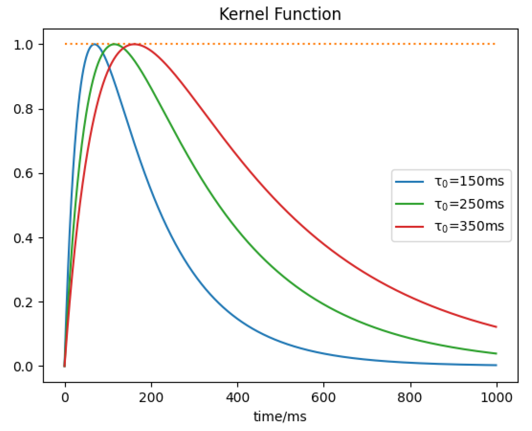
As is shown in Figure 1, the kernel function rises gradually before it reaches the maximum. After that, it decays more slowly than it rises. This feature of a slow rise and slower decay enables the kernel function to imitate the true circumstance of animal neurons. The figure also shows different shapes of the kernel function with different time constants. In all three functions, τ₁ is set to be τ₀/4, and the maximums of the three functions are all normalized to 1. The maximum of the kernel function comes first when τ₀ = 150 ms and comes last when τ₀ = 350 ms. With τ₀ getting larger, the rising period gets longer and the rising and decaying rates get slower.

Second, an exponential function is used to describe the membrane’s response to the DC stimulus. Here, the DC stimulus is regarded as a constant so that the non-spike potential of the membrane will regress to a constant. When there is no DC stimulus, the non-spike potential of the membrane will regress to 0.

Combining the two parts, the evolution of membrane potential is:

$$V_{mem}(t)={\displaystyle \sum _i{W}_i{\displaystyle \sum _{t_k<t}K(t-t_k)}}+V_{regress}(t),$$

(2)

where W_i is the weight value of the synapse linking two neurons.

In the firing part, the threshold of the membrane potential is set to be a constant ϑ. When V_mem crosses the threshold from small to large, the neuron fires a spike. In the meantime, all the accumulated electronic charges are cleared out and the membrane potential is reset at V_reset to imitate the true discharging process. V_reset is smaller than 0 and is a non-spike potential, so it will regress to 0, influenced by DC stimuli even when there is no DC stimulus.

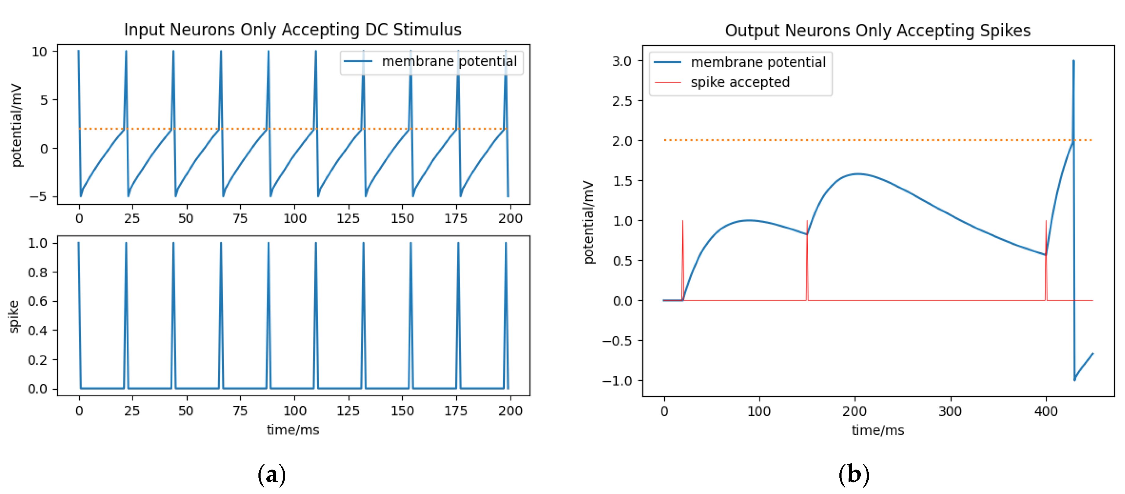
In this paper, input neurons are separated from output neurons by the difference of these two membrane potential resources. Neurons that only accept DC stimuli are input neurons. Influenced by the DC stimulus, the membrane potential rises by exponential regression. Furthermore, limited by the voltage threshold, input neurons keep generating spikes regularly and the membrane potential recovers from V_reset all the time (see in Figure 2a).

Neurons that only accept spikes are output neurons. The membrane potential of output neurons can be simplified as:

$$V_{out}(t)={\displaystyle \sum _i{W}_i{\displaystyle \sum _{t_k<t}K(t-t_k)}},$$

(3)

without considering the reset part. Influenced by the kernel function, the output neurons fire a spike only during the rising period of the last received spike (before the output neurons fire a spike; see in Figure 2b) because the threshold of the membrane potential is only triggered when the membrane potential increases.

Assuming that an output neuron accepts a series of regularly generated spikes (the interval period between spikes is a constant), stimuli applied to the membrane will be stable and persistent so that the interval period between an output neuron’s spikes will not change. And as a result, the first spike that an output neuron fires is carrying all the information with it and the first spike time is adequate to deliver the information.

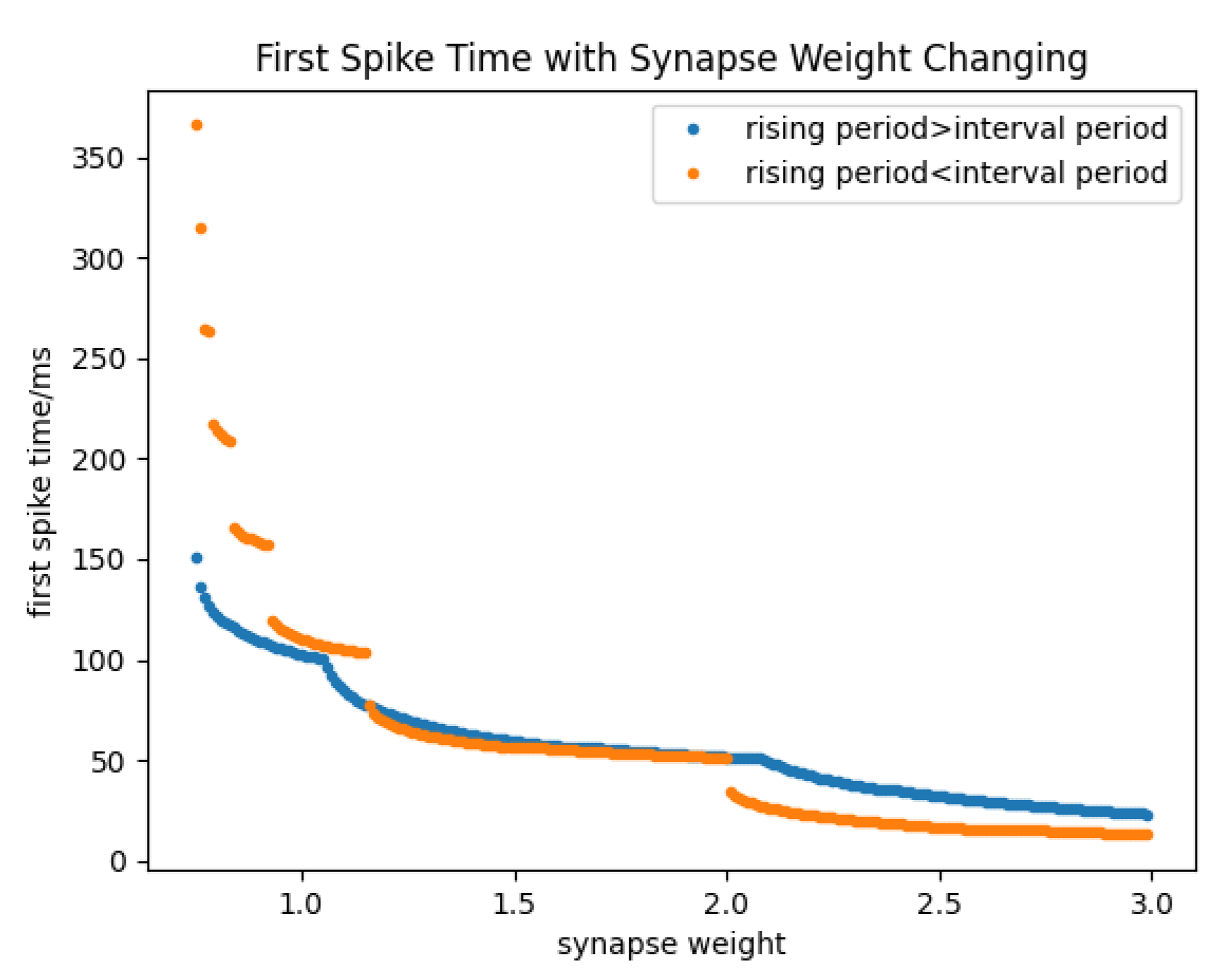
The differential relationship between synaptic weight and first spike time needs to be discussed if the first spike time is chosen to be the neuron’s output. Figure 3 shows the process of the first spike time getting close to zero with the synaptic weight increases. Those points where the rate of the first spike time’s decaying largely changed are influenced by external spikes reaching the membrane.

The relationships between W_i and the time of the output neuron first firing a spike could be different depending on the relationships between the rising period of the kernel function and the interval period between received spikes. Figure 3 also shows the different situations in whether the rising period of the kernel function is larger than the interval period between received spikes or not.

As shown in Figure 3, when the rising period of the kernel function is larger than the interval period between received spikes, the time of the output neuron’s first spiking changes continuously. Otherwise, the first spike time changes discontinuously, which means the time axis cannot be fully covered. The reason for this situation is that the output neurons fire a spike only during the rising period of the last received spike. When the rising period is smaller than the interval period, the kernel function caused by the last received spike would decay before a new spike reaches the membrane and produces a new rise tendency. In this paper, the rising period is set to be larger than the interval period in order to guarantee full use of the time axis.

3. Actor-Critic Network Structure with TD

3.1. The Actor-Critic Network

The actor-critic algorithm combines the policy-based method and the value-based method, so it needs two nets to implement these two ways. One is from state to actor, where the actor will choose an action to take based on probability; the other is from state to critic, where the critic judges the value of the action chosen by the actor. As is shown in Figure 4, the actor-critic network consists of state neurons (in blue), critic neurons (in green) and action neurons (in orange).

Each state neuron represents a state. When a state is chosen (the state neuron is surrounded by a red circle in Figure 4), the corresponding state neuron would accept a constant DC stimulus. Since state neurons only accept DC stimuli, state neurons are all input neurons. Therefore, the chosen state neuron will generate a series of regular spikes and these spikes will be delivered to all critic neurons and action neurons.

Critic neurons generate the value function. Since critic neurons only accept spikes fired by state neurons through the red lines in Figure 4, critic neurons are all output neurons. Therefore, the value function is designed to relate to the first spike time of each critic neuron. To match the value function with the weight values, the value function is designed to have a contrasting increasing tendency to the first spike time. Here, the exponential function on the negative values of the spike times t_j is used:

$$\upsilon (S,\omega )=e^{-t_j}.$$

(4)

Each action neuron represents an action. Similar to critic neurons, action neurons are all output neurons, too. They only accept spikes fired by state neurons through the blue lines in Figure 4. The softmax function is used on the negative values of the first spike times t_l to represent the probability of choosing each action neuron [26]. The equations are:

$$q_l=e^{-t_l},$$

(5)

$$p_l=\frac{q_l}{{\displaystyle \sum _{m=1}^M{q}_m}}.$$

(6)

The action of which the corresponding action neuron fires the first spike of all action neurons is chosen. When one of the action neurons is chosen, a reward signal will be generated and delivered to all critic neurons.

3.2. Update the Value Function

If δ is the temporal difference and ω_ij is the weight value of the synapse that links state neuron i and critic neuron j, then the updating process of the value function is:

$$\delta \leftarrow R(S^{\prime })+\gamma \upsilon (S^{\prime },\omega )-\upsilon (S,\omega ),$$

(7)

$$\omega \leftarrow \omega +\beta \delta {{\displaystyle \nabla }}_{\omega }\upsilon (S,\omega ).$$

(8)

Assuming that state neuron i is the currently chosen state neuron, we only need to calculate ∂υ(S,ω)/∂ω_ij when calculating ${{\displaystyle \nabla }}_{\omega }\upsilon (S,\omega )$, since the other state neurons have no generations. The result is:

$$\frac{\partial \upsilon (S,\omega )}{\partial {\omega }_{ij}}=\frac{\partial e^{-t_j}}{\partial t_j}\cdot \frac{\partial t_j}{\partial {\omega }_{ij}}=-e^{-t_j}\cdot \frac{\partial t_j}{\partial {\omega }_{ij}}.$$

(9)

Next, ∂t_j/∂ω_ij is calculated. Now that critic neurons are output neurons, the membrane potential of critic neuron j can be expressed as:

$$V_j(t)={\displaystyle \sum _i{\omega }_{ij}{\displaystyle \sum _{t_k<t}K(t,t_k)}}={\omega }_{ij}{\displaystyle \sum _{t_k<t}\frac{1}{\kappa }\left[\exp \left(-\frac{t-t_k}{{\tau }_0}\right)-\exp \left(-\frac{t-t_k}{{\tau }_1}\right)\right]}.$$

(10)

If ϑ is the firing threshold of membrane potential and t_j is the first firing time of critic neuron j, then $V_j(t_j)=\vartheta$ can be determined, and

$${\omega }_{ij}{\displaystyle \sum _{t_k<t_j}\frac{1}{\kappa }\left[\exp \left(-\frac{t_j-t_k}{{\tau }_0}\right)-\exp \left(-\frac{t_j-t_k}{{\tau }_1}\right)\right]}=\vartheta .$$

(11)

The partial derivative of ω_ij on both sides of the equation can be determined:

$$\frac{\partial t_j}{\partial {\omega }_{ij}}=\frac{\kappa \vartheta }{{\omega }_{ij}^2}\frac{1}{{\displaystyle \sum _{t_k<t_j}\left[\frac{1}{{\tau }_0}\exp \left(-\frac{t_j-t_k}{{\tau }_0}\right)-\frac{1}{{\tau }_1}\exp \left(-\frac{t_j-t_k}{{\tau }_1}\right)\right]}}.$$

(12)

3.3. Update the Policy

Assuming π(A|S,θ) is the probability of choosing action A and θ_il is the weight value of synapse that links state neuron i and action neuron l, the updating process of the value function is:

$$\theta \leftarrow \theta +\alpha \delta {{\displaystyle \nabla }}_{\theta }\log \pi (A\left|S,\theta \right.).$$

(13)

According to (6),

$$\pi (A\left|S,\theta \right.)=p_l=q_l/{\displaystyle \sum _{m=1}^M{q}_m}.$$

(14)

Assuming that state neuron i is the currently chosen state neuron, we only need to calculate ∂logπ(A|S,θ)/∂θ_il when calculating ${{\displaystyle \nabla }}_{\theta }\log \pi (A\left|S,\theta \right.)$ since the other state neurons have no generations. The result is:

$$\frac{\partial \log \pi (A\left|S,\theta \right.)}{\partial {\theta }_{il}}=\left\{\begin{array}{ll}-(1-p_l)\cdot \frac{\partial t_l}{\partial {\theta }_{il}},\hfill & chosen\hfill \\ p_l\cdot \frac{\partial t_l}{\partial {\theta }_{il}},\hfill & otherwise\hfill \end{array}\right..$$

(15)

The calculating process of ∂t_l/∂θ_il is the same as that of ∂t_j/∂ω_ij, which is:

$$\frac{\partial t_l}{\partial {\theta }_{il}}=\frac{\kappa \vartheta }{{\theta }_{il}^2}\frac{1}{{\displaystyle \sum _{t_k<t_l}\left[\frac{1}{{\tau }_0}\exp \left(-\frac{t_l-t_k}{{\tau }_0}\right)-\frac{1}{{\tau }_1}\exp \left(-\frac{t_l-t_k}{{\tau }_1}\right)\right]}}.$$

(16)

The actor-critic network structure and the update formulas using temporally encoded information is provided. The actor-critic network structure with TD is shown as Algorithm 1.

Algorithm 1 Actor-critic network structure with TD

Input: the initial parameters of actor-critic network ${\mathsf{\theta }}^{\left(0\right)}$ and ${\mathsf{\omega }}^{\left(0\right)}$; the parameters of the network after the ith update ${\mathsf{\theta }}^{\left(i\right)}$ and ${\mathsf{\omega }}^{\left(i\right)}$; input signal; the maximum running time time_end; the learning rate of actor-critic network ${\mathsf{\alpha }}_{\mathsf{\theta }}>0, {\mathsf{\alpha }}_{\mathsf{\omega }}>0$;

1: $\mathrm{Initialize} \mathrm{the} \mathrm{running} \mathrm{time} time=0; \mathrm{the} \mathrm{state} S_t$.

2: Repeat

3:  time←time + 1

4:  Input signal[time] to the actor-critic network

5:  if actor network generates action signals then

6:     $\mathrm{Calculate} {\nabla }_{\mathsf{\theta }}log\mathsf{\pi }\left(A|S,\mathsf{\theta }\right)$ based on the selected action A

7:     $\mathrm{Update\; the\; state} S^{\prime } \text{and the reward signal} R_{t+1}$

8:  end if

9:  if critic network generates value function then

10:    Calculate ${\nabla }_{\mathsf{\omega }}\upsilon \left(S,\mathsf{\omega }\right)$

11:  end if

12:  if value function gradient and policy gradient have been solved then

13:    $\mathsf{\delta }\leftarrow R\left(S^{\prime }\right)+\mathsf{\gamma }\upsilon \left(S^{\prime },\mathsf{\omega }\right)-\upsilon \left(S,\mathsf{\omega }\right)$

14:    $\mathsf{\omega }\leftarrow \mathsf{\omega }+\mathsf{\beta }\mathsf{\delta }{\nabla }_{\mathsf{\omega }}\upsilon \left(S,\mathsf{\omega }\right)$

15:    $\mathsf{\theta }\leftarrow \mathsf{\theta }+\mathsf{\alpha }\mathsf{\delta }{\nabla }_{\mathsf{\theta }}log\mathsf{\pi }\left(A|S,\mathsf{\theta }\right)$

16:    $S\leftarrow S^{\prime }$

17:  end if

18: Until time > time_end

4. Results and Discussion

4.1. Gridworld Task

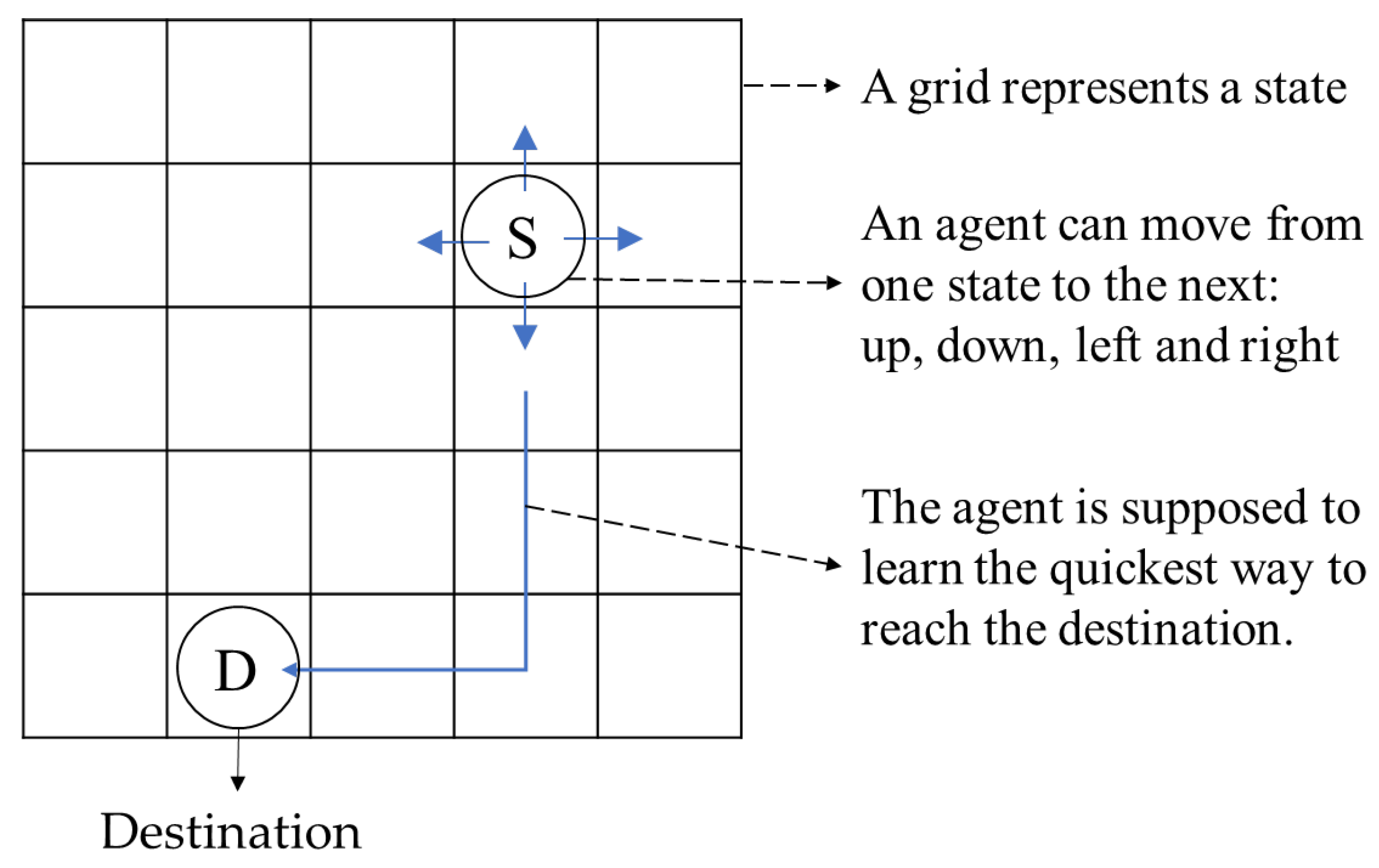
The algorithm is tested in a gridworld task. The gridworld is a good approximation of real world. The environment is divided into regular grids so that the relationship between the environment and the agent is shown clearly. It is a common test for reinforcement learning algorithms since it provides a good way to implement a finite Markov decision process. In this case, it is convenient to use the gridworld to show the agent’s states. The gridworld is a map on which an agent can move from one state to the next by taking four different actions: up, down, left and right (see in Figure 5). A random state S_d is selected as the destination (state D in Figure 5).

Since the agent can only take four directions, the distance on the map is defined as vertical distance plus horizontal distance, which is shown as follows:

$$d(S,S^{\prime })=\left|x-x^{\prime }\right|+\left|y-y^{\prime }\right|,$$

(17)

where S = (x,y) and S′ = (x′,y′). x, y and x′, y′ are integers between 1 and 5.

The agent is supposed to learn the quickest way to reach the destination. To ensure that, the reward at the destination is one and the reward at other states is zero. In the meantime, the value function at the destination is set to zero.

To measure the agent’s performance, the latency of the agent moving from the initial state to the destination state is designed. Assuming n is the number of moves that the agent takes from the initial state to the destination state, latency is defined as:

$$latency=n-d(S_{initial},S_d).$$

(18)

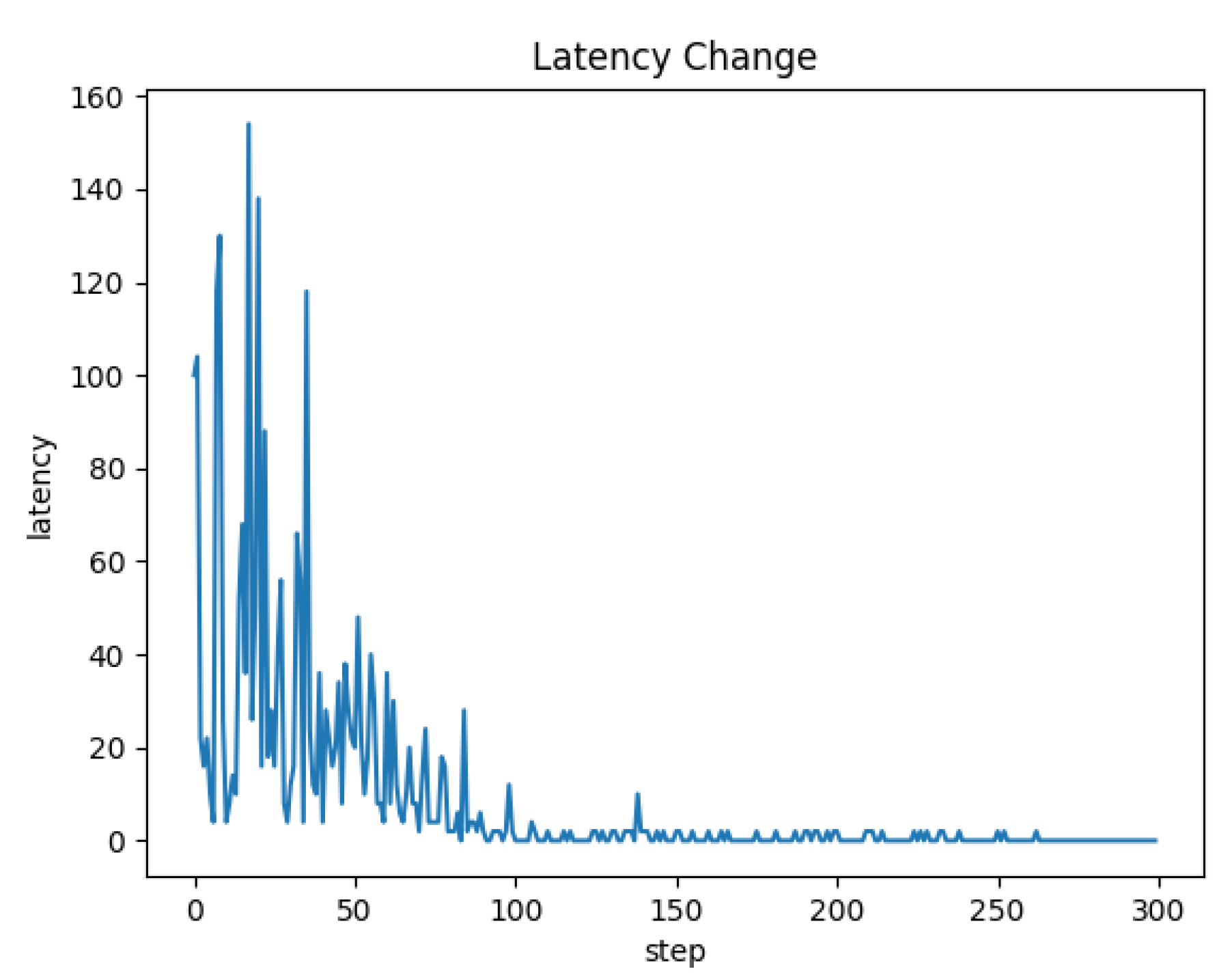
When the agent reaches the destination, the initial state is updated with a random state on the map. During the learning process, each state has a latency value. We choose one state’s latency value as a target, for example, state S in Figure 5. The agent won’t stop learning until the maximum is small enough. Figure 6 shows the latency change during learning. When the latency converges to zero, the quickest way from state S to state D is found.

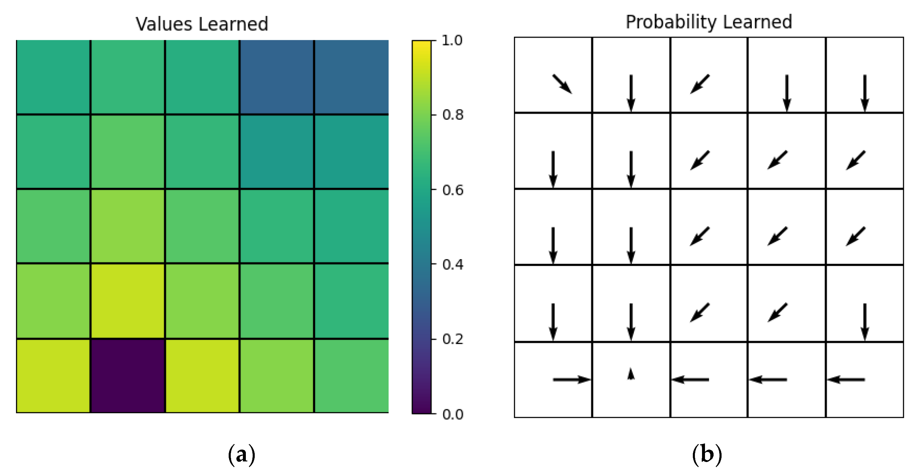
After an agent’s learning, a color map is used to show states’ values in Figure 7a. With states getting farther away from the destination, states’ values decay. Since we set γ = 0.9 in Equation (7), under the ideal circumstance the states’ values would be:

$$V_{ideal}(S)={0.9}^{d(S,S_d)}.$$

(19)

A root mean square error can be obtained to describe the performance of value learning:

$${\sigma }_V=\sqrt{\frac{{\displaystyle {\sum }_S(V(s)-V_{ideal}(s)}{)}^2}{N_S}}.$$

(20)

Here, N_S is the number of states. For the values showed in Figure 7a, σ_V = 0.05347. Considering the computing error, this result is acceptable.

A probability arrow $\overrightarrow{p}(S)$ is used for each state to judge the agent’s policy learning, which is:

$$\overrightarrow{p}(S)=\left(\begin{array}{c}\pi (up\left|S\right.)-\pi (down\left|S\right.)\\ \pi (left\left|S\right.)-\pi (right\left|S\right.)\end{array}\right).$$

(21)

The probability arrow map can show us the agent’s learning achievements in a direct way.

Except for the destination, all states’ probability arrows point to the states which have the largest values in their neighbors, so that the quickest way from each state to the destination is found. However, a part of the probability arrows is largely different from the ideal circumstance. For example, the three downward arrows in the first left row completely abandon the probability to take the right direction, which is obviously not ideal. This situation may be related to the synaptic weight change when the synaptic weight is small enough. Overall, the synaptic weight change tends to be larger when it is smaller. Therefore, it is possible that the synaptic weight gets too small to make the output neuron fire a spike if only another action with an advantage is chosen continuously. In that way, although this action is also advantageous, it might be abandoned.

4.2. UAV Flying through Window Task

The current algorithm is then tested in a UAV flying through a window task by simulation on XTDrone platform [31,32]. In this experiment, we keep the 25 states in the gridworld task. Based on the relative position between the UAV and the window and the window’s position in the image that the UAV can detect, we establish a corresponding relationship between the UAV’s detection and a 5 × 5 grid map. As shown in Figure 8, the four red squares on the top represent the UAV’s detection. The four white squares represent the window, and they do not have to be an appropriately sized square.

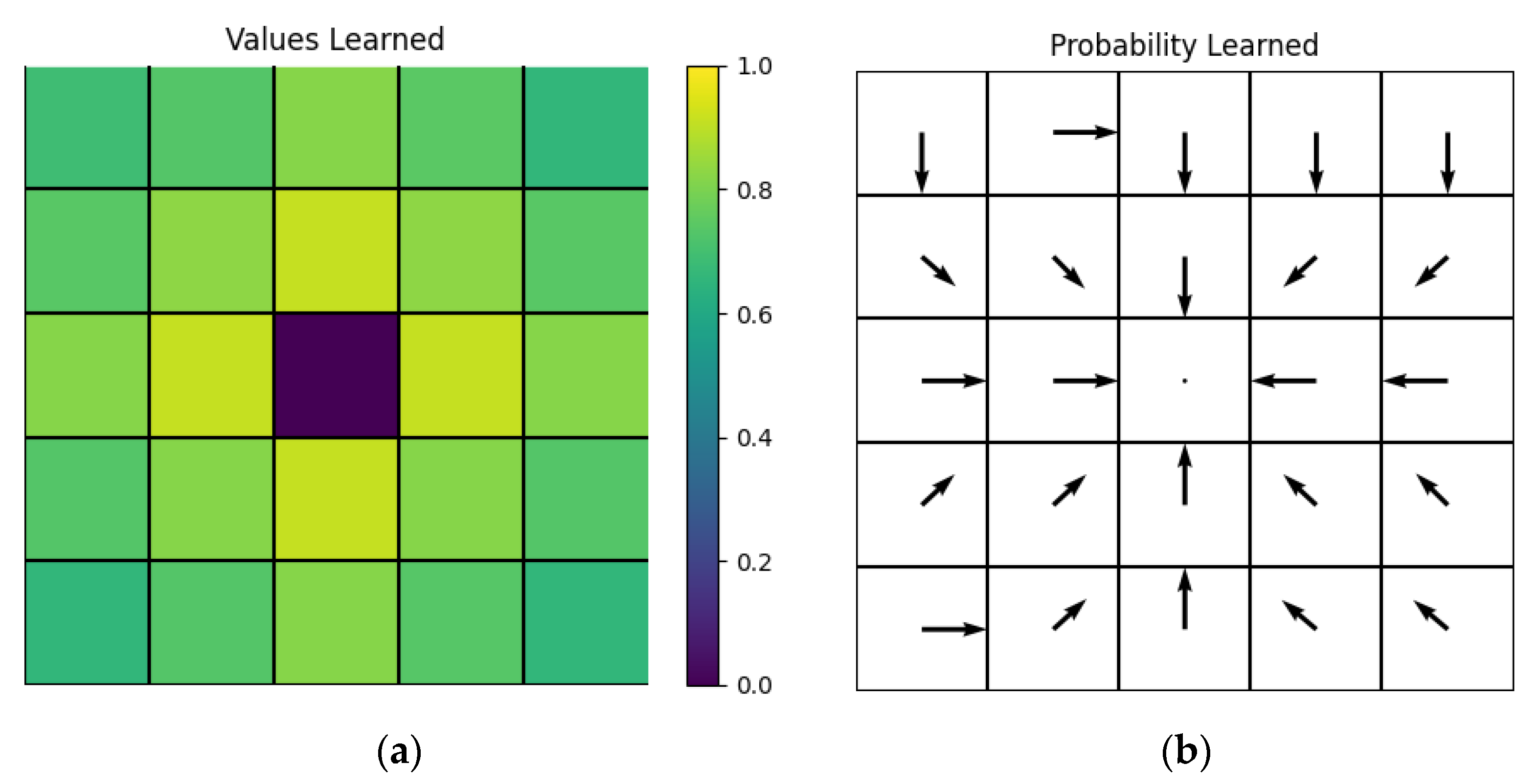
The window’s position is chosen at the center of the grid map. In the UAV’s detection, when the window shows at the bottom-right corner of the image, we transfer it to the center of the grid map and set the UAV’s state at the up-left corner of the grid map. This way, we reset the destination state to the center point of the grid map in Section 4.1 and operate another learning. The results of the values’ color map and probability arrow map are shown in Figure 9.

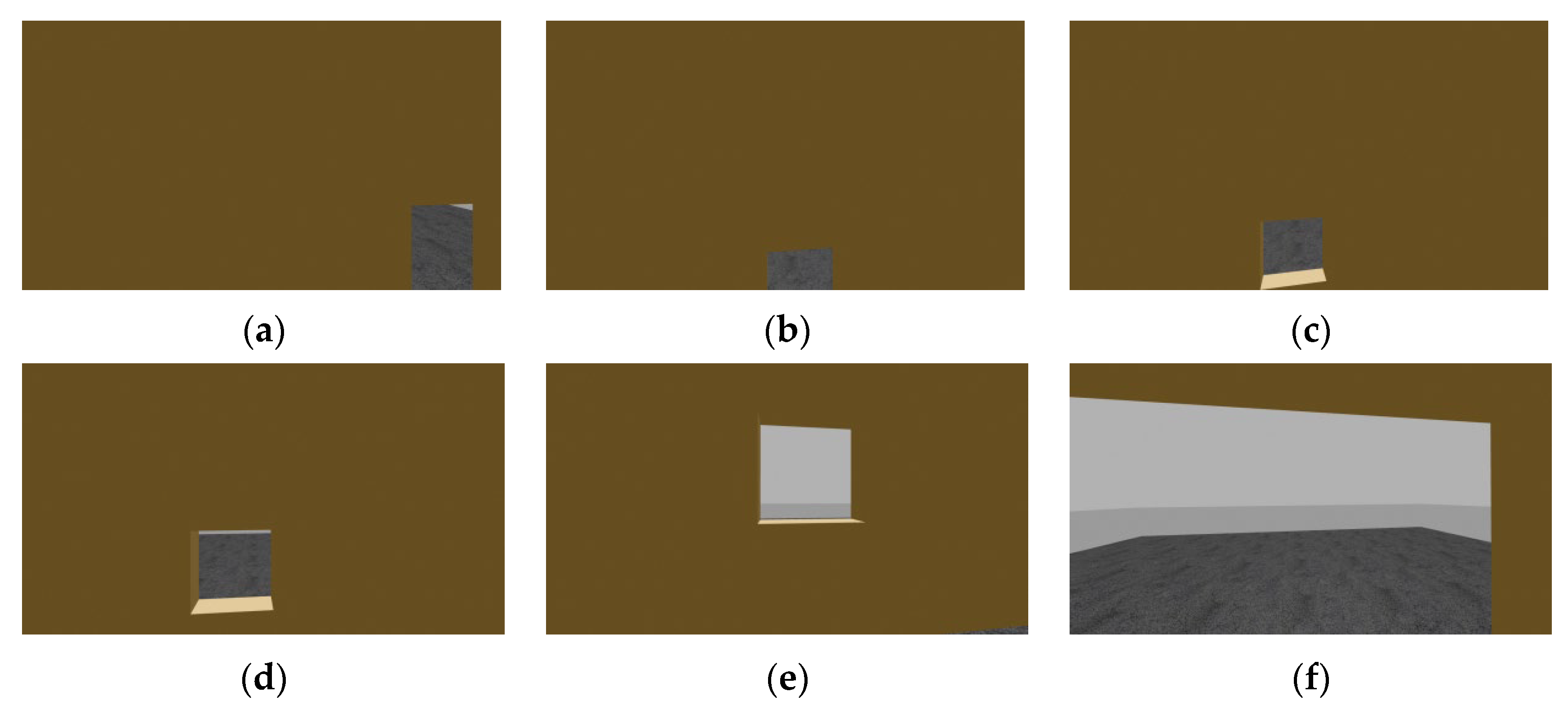
In the simulation environment, we set a wall and a square window. We use edge detection to preprocess the camera image to find the window’s position, and then transfer it into the grid map to distinguish the state. Finally, the UAV takes an action to aim at the window.

We put the UAV at a random position in front of the wall and let it make a decision to fly through the window. A series of actions that the UAV takes is shown in Figure 10. Obviously, the UAV takes the quickest way to reach the center point in the grid map as trained, which means the UAV takes the quickest way to get to the position in front of the window where it can aim at and fly through the window.

4.3. UAV Avoiding Flying Basketball Task

The task of UAV fast obstacle avoidance is conducted to verify the performance of the algorithm. We choose a standard basketball with a radius of about 12.3 cm. The basketball is thrown from 3–5 m in front of the UAV and the speed is 3–5 m/s. The sensor selected by the UAV is a monocular camera with a frame rate of 31 fps. The simulation and the true flight test are based on the above simple experimental settings. The task does not consider the dynamic background due to the differential encoding of the camera input. In the dynamic background, the decision accuracy will be affected. Moreover, in order to facilitate the training and calculation of the network, the hovering UAV can only choose three actions, left, right and hovering, to complete the obstacle avoidance task (see in Figure 11). The maximum flight speed of the UAV is limited to 3 m/s during the experiment.

In this experiment, the basketball’s flight trajectory will mostly pass through the initial position of the UAV. In order to prevent a reduction in the training effect, the UAV should be kept in its initial position as much as possible and return again after avoiding.

Based on the above characteristics, the goal of the training network is to prolong the survival time of the UAV in the initial position and keep hovering. Therefore, we assume that the reward signal has the following characteristics:

• The longer the UAV survives, the greater the reward;
• The farther the UAV is from the initial position, the smaller the reward;
• If the UAV fails to avoid the flying basketball, it will be punished.

Therefore, the basic reward $R_0$ that varies with the distance of the UAV from the initial position is designed. Note that the distance between the current position of the UAV and the initial position is $d$, and the time that the drone has survived so far is $t_s$. In the case of the right decision, the reward signal would be:

$$R={{\displaystyle \sum }}_{i=0}^{t_s/\Delta t}{R}_0\left(d,i\Delta t\right)$$

(22)

$$R_0\left(d,i\Delta t\right)=R_0\left(0,t\right)\exp \left(-\frac{d}{D}\right)$$

(23)

where $D$ is a constant representing the level to which the reward signal decreases with the distance.

If the wrong decision is made, the UAV will be punished. The signal is defined as:

$$R=-p{R}_0\left(d,t\right)$$

(24)

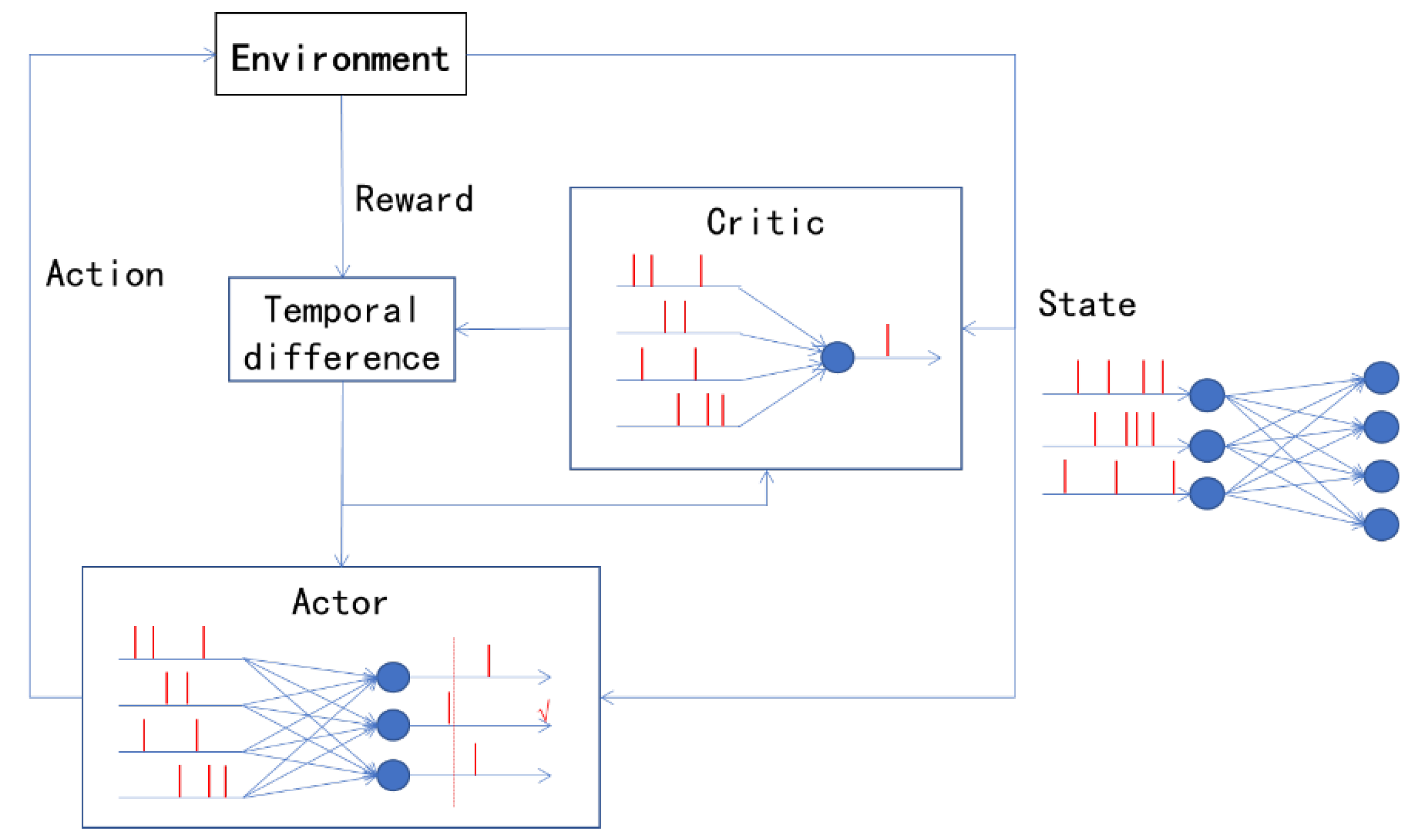
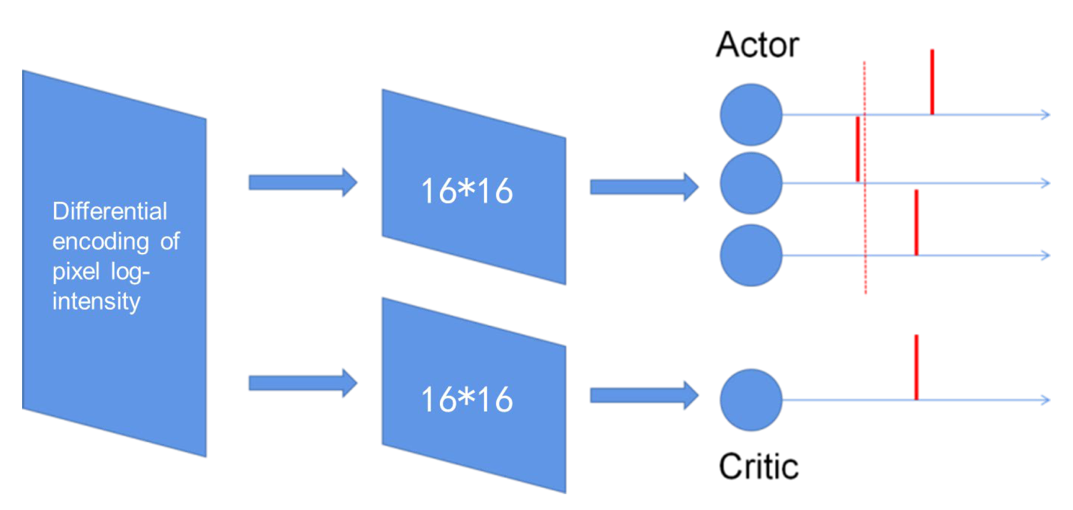
where $p$ is the penalty factor and is large enough that the reward previously obtained by the UAV is completely cancelled. In the simulation environment, dynamic obstacles are designed to train spiking neural networks in the XTDrone platform. The structure of the spiking AC network is shown in Figure 12. The number of neurons in the input layer is the same as the number of pixels in a monocular camera. The input camera data are processed by differential coding and the neuron corresponding to the pixel with a significant change in brightness will generate a pulse. The hidden layer of the actor network and critic network consists of 16*16 spiking neurons. While the output layer of the actor network has three neurons, representing left, right and hovering, the output layer of the critic network has one neuron, which represents the state value function.

The initial parameters are selected before training. The key parameters are given in

Table 1. Summary of parameters.

Notation	Definition	Value
${\mathsf{\tau }}_0$	The membrane potential integration constant of the kernel function	150
$\mathsf{\zeta }$	Neuron firing threshold	50
$u_{rest}$	Neuron resting potential	0
$u_r$	Neuron recovery potential	−15
$\mathsf{\beta }$	Neuron firing probability	50
${\mathsf{\alpha }}_{\mathsf{\theta }},{\mathsf{\alpha }}_{\mathsf{\omega }}$	Update rate	0.01
$\mathsf{\gamma }$	Discount factor	0.9
$\mathsf{\lambda }$	Damping decrement	0.8
$\Delta L$	Log-intensity threshold	0.25
$R_0\left(0,t\right)$	Initial reward	50
$D$	Reward decay rate	3
$p$	Penalty factor	1000

.

Among them, the first nine parameters are selected based on [30]. While the other parameters are ultimately selected by testing several times. The actor-critic network parameters $\mathsf{\theta }$ and $\mathsf{\omega }$ are initialized randomly. These initial parameters execute the iterative optimization during the training. After that, the true flight test is conducted using the trained actor network parameters.

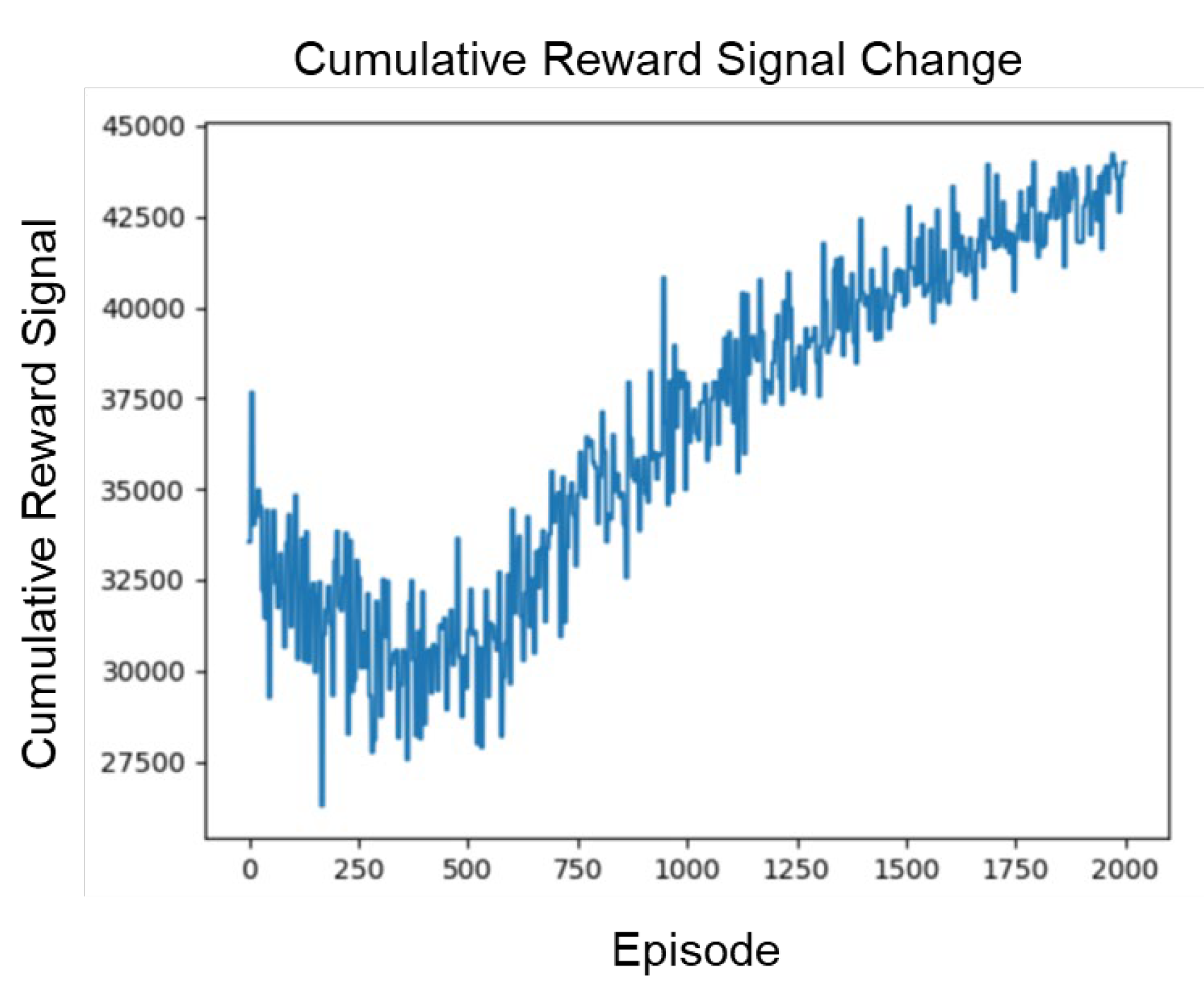
During the simulation, the overall time of the spiking neural network is discrete, and the time step is one millisecond. A throw of the ball is regarded as one episode. Generally, the length of one episode is about one second. Overall, the cumulative reward signal obtained by the UAV is on the rise, indicating that the training is effective and the survival time is increasing (see in Figure 13).

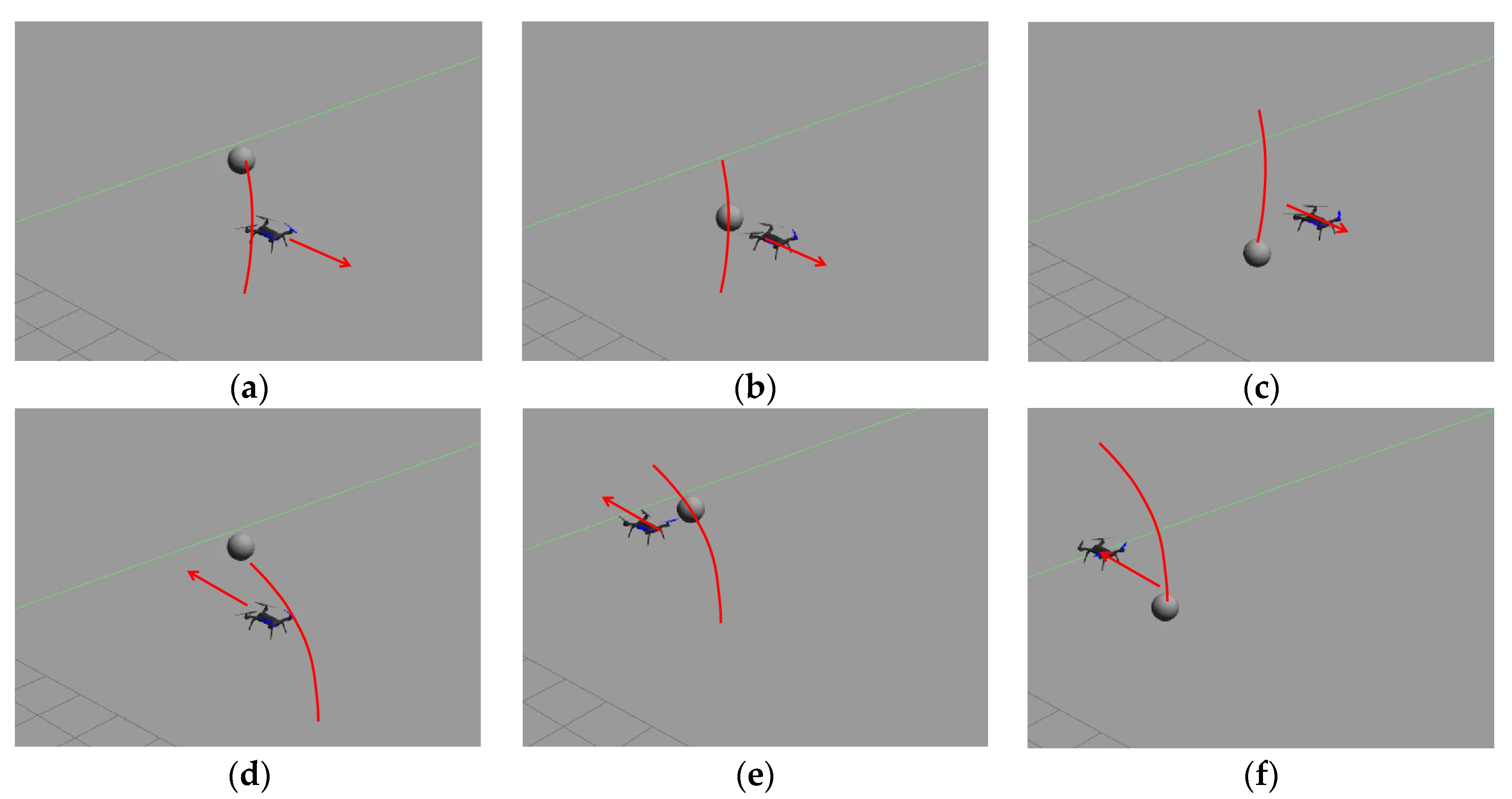
Several typical scenarios in which the UAV avoids the flying basketball during the simulation experiment are shown in Figure 14.

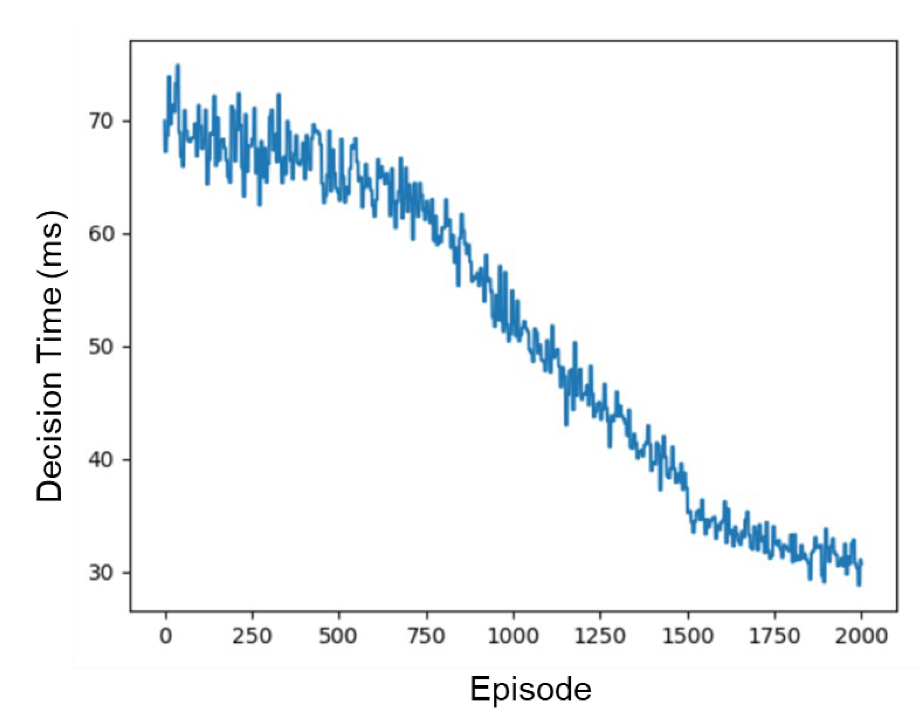
In order to facilitate the optimization and improvement of the network, small parameters are selected for initialization. Therefore, at the beginning of training, it takes a long time for the UAV to make a decision. The time it takes for the UAV to make a decision then gradually decreases during the training (see in Figure 15). At the end of the training, the average time spent by the UAV to make a decision drops to 30.7 milliseconds.

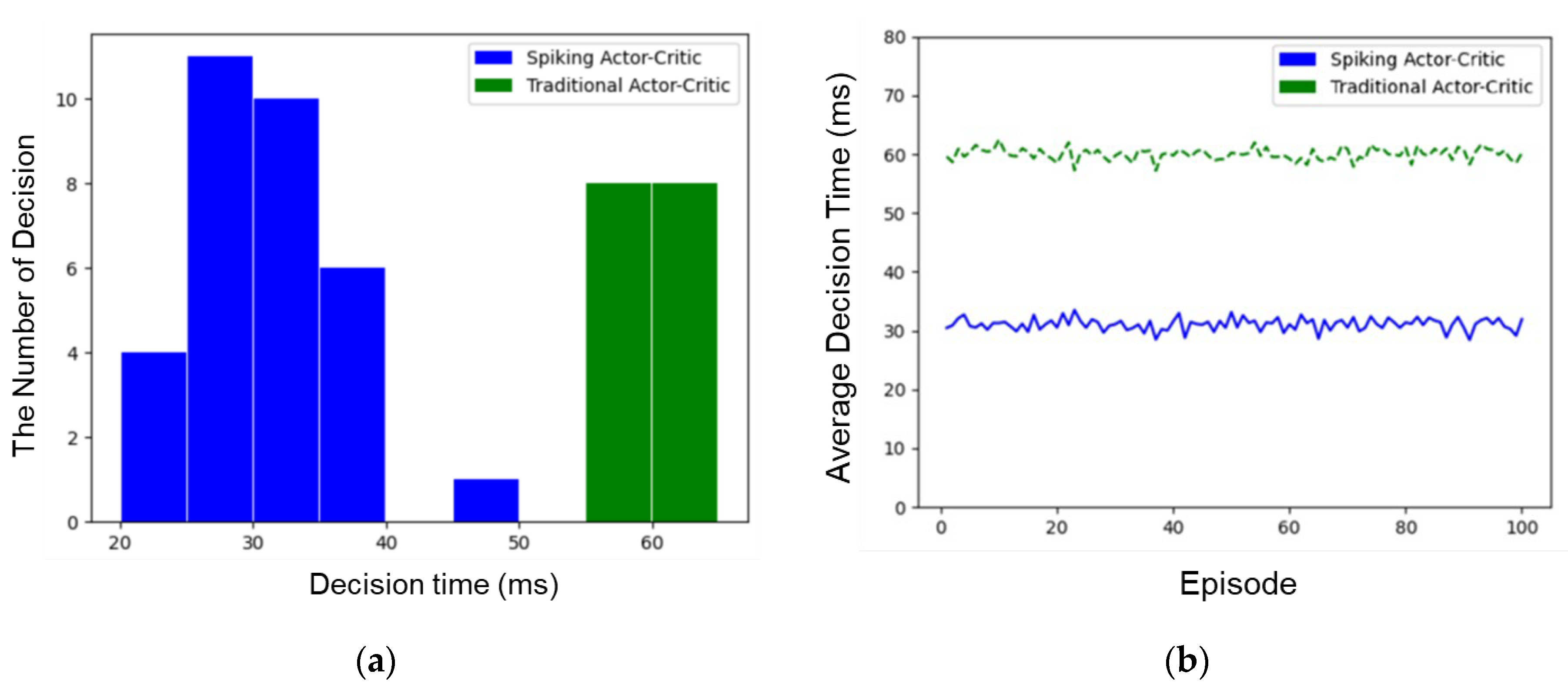
Comparative experiments with traditional AC networks are also carried out to verify the rapidity of the algorithm. One hundred basketball-avoiding experiments were performed in the simulation platform. The UAV used the spiking AC algorithm and the traditional AC algorithm to make decisions, respectively. Figure 16a shows the distribution of decision times for one of the basketball avoidances. It is noted that the decision time of the UAV using the spiking AC network is mainly concentrated in the interval of 25 ms to 35 ms, while the decision time of using the traditional AC network is concentrated in the interval of 55 to 65 milliseconds. The decision-making algorithm proposed in this paper is significantly faster, so the number of decisions in one episode is also significantly larger. Figure 16b shows the average decision time for one hundred basketball avoidance experiments. As shown in the figure, the average decision-making time of the UAV using the algorithm proposed in this paper is about 30 milliseconds, while the average decision-making time of the UAV based on the traditional AC network is about 60 milliseconds. Therefore, the UAV decision-making algorithm proposed in this paper greatly speeds up the UAV’s decision-making.

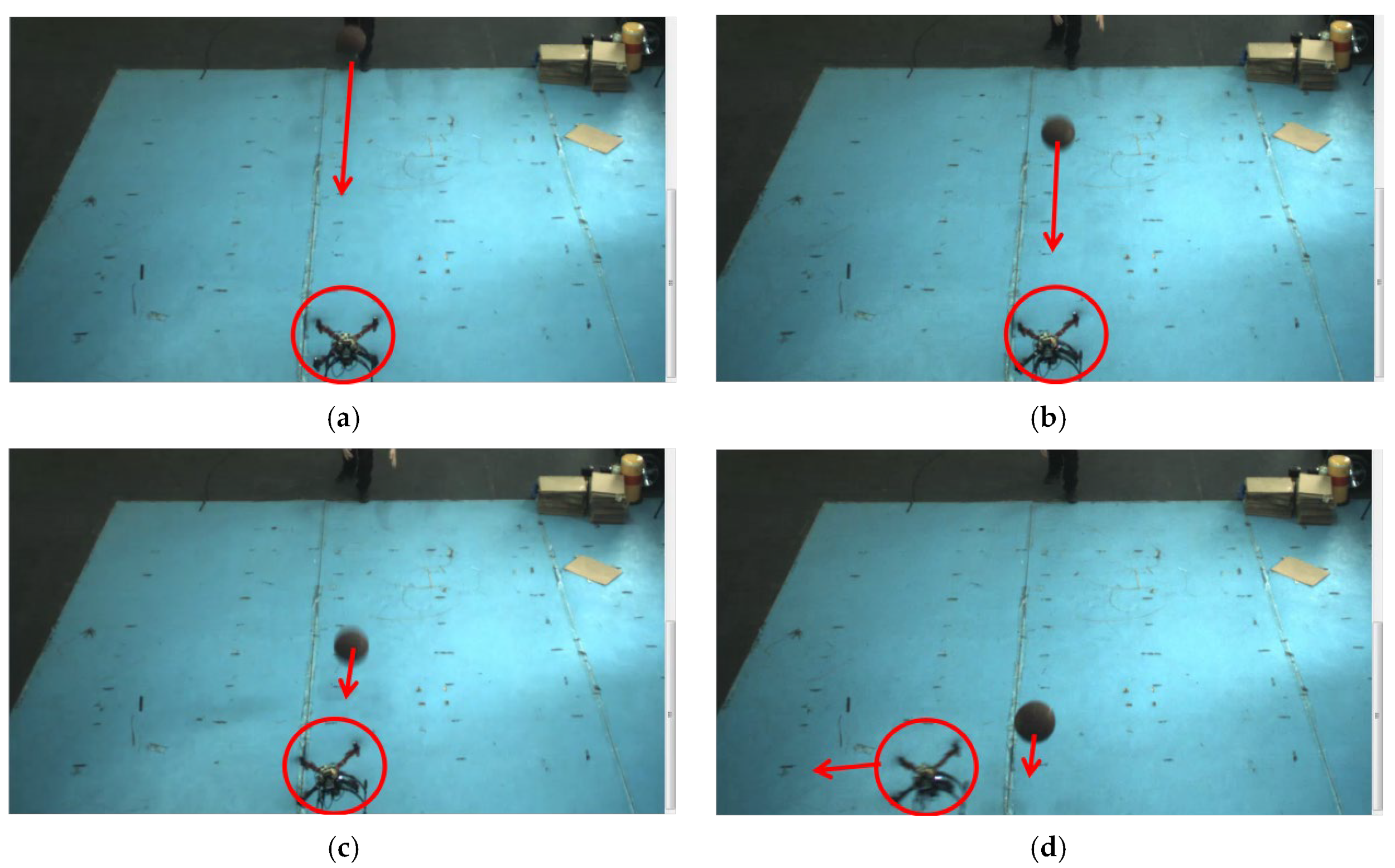
The algorithm is then tested through the actual flight test of the UAV avoiding flying basketballs. A F450 quadrotor UAV carrying the TX2 computing platform is used to conduct the task and the maximum flight speed of it is 3 m/s. A scene of the experiment is shown in Figure 17. In this experiment, the basketball is thrown from 3–5 m on the left front of the UAV. When the basketball approaches, the UAV makes a decision to fly to the left and successfully avoids collision.

We repeated the above experiment 100 times and the success rate of obstacle avoidance was 96%. It can be observed that the randomness of the actor network does not have a significant impact on the UAV’s decision-making. The average decision time of 100 times is 41.3 ms, which is slightly longer than the simulation experiment. The reason may be that the processing of camera data cannot be ignored in the actual flight, slowing down the efficiency of the network. The scripts can be found in the Supplementary Material.

4.4. Discussion

The purpose of this paper is to explore a new method of decision-making which is resource-saving while not performance-limiting. The method proposed in this paper is to use a spiking neural network, for it consumes low power and has the potential to accelerate the process of decision-making.

To realize the spiking neural network’s potential, temporal encoding is essential. So far, temporal encoding has been introduced to supervised learning of spiking neural networks because back propagation would be possible for SNN with the help of temporal encoding. It is natural to ask if it could be used in reinforcement learning, and that leads to this paper’s main idea. In this paper, we execute a simple test and do not use temporal encoding all over the network structure. For input neurons, we still use rate-coded neurons, which definitely restrict the scale of state space. Next, we would like to try to use temporal coding to design a whole new structure, as we are trying to encode the input information in the temporal domain and figure out the how that would influence decision-making.

5. Conclusions

This study provides a lightweight decision-making method using a simple improved leaky integrate-and-fire (LIF) model and small-scale spiking actor-critic network with only 2–3 layers to realize complex decision-making tasks such as UAV window crossing and avoiding dynamic obstacles. The improved leaky integrate-and-fire (LIF) model is used to describe the behavior of a spike neuron, and the actor-critic network structure and the update formulas using temporally encoded information are provided. A temporal coded spike neural network RL method is tested in the simulation of decision-making in a 5 × 5 grid map task, the UAV flying through a window task and avoiding flying basketballs task. An actual flight test of the UAV avoiding flying basketballs is conducted. The success rate of obstacle avoidance is 96% and the average decision-making time is 41.3 ms. These results show the effectiveness and accuracy of the temporal coded spiking neural network RL method and demonstrate the advantages of faster decision-making and a stronger biological interpretability than the traditional AC network. This study provides an effective solution for the rapid decision-making of unmanned systems.