Abstract
Although it possesses the capabilities of both anti-contamination and rapid response, the deflector jet servo valve is still confronted with the issue of weak performance robustness, usually manifesting as considerable uncertainty of the product pressure indices. To elaborate on the complex internal mechanism of deflector jet valves and figure out the origins of performance fluctuations, a three-dimensional mathematical model of the deflector jet pilot valve is constructed, in which a series of assumptions are presented to apply specific theorems to different regions of the flow field. Numerical simulations and experiments show that this theoretical system can provide a distinct and logical explanation for both the internal flow distribution and the external performance of the servo valve. On this basis, the causes of performance fluctuations are discussed, concerning the installation error of the deflector and the machining error of the shunt wedge. Calculations show that the latter can bring about remarkable performance variation. Quantificationally, a 10 micron width error of the shunt wedge will induce 7.4% and 3.6% drifts of the receiver pressure and the pressure gain, respectively. However, further analyses confirm that a decrease in the deflector jet distance will lead to dramatic deterioration of the valve’s susceptibility to errors. Hence, it is concluded that to enhance the performance robustness of servo valve products, the machining accuracy of the shunt wedge and non-negative errors of the deflector jet distance should both be guaranteed.
1. Introduction
With the advantages of rapid response and anti-contamination, the deflector jet servo valve (DJV) has become a promising hydraulic control component in aerospace engineering, marine technology, and other industries. Nevertheless, DJV research is still confronted with ambiguity of the working mechanism and cannot explain the great uncertainty of product performance.
A comprehensive review of electro-hydraulic servo valves was provided in Tamburrano et al., which pointed out that two-stage valves were usually in the form of a pipe jet or a deflector jet [1]. Early DJV research originated from analyses of the jet pipe valve, and most methodologies were concerned with numerical simulation. Initially, a finite element model was built to study the fluid–structure interaction effect on the equilibrium state of the jet pipe valve [2]. Meanwhile, a model with consideration of the dynamics of fluid flows, flow reaction forces, and friction forces was established to obtain a more accurate representation of the servo valve [3]. Additionally, then, it was reported that the roughness of the impact surface has an influence on the flow regime, which was based on a RANS-based simulation [4]. With the same method adopted, mechanisms of different parameters acting on the jet pipe valve were explored [5,6,7].
Compared to the jet pipe valve, the DJV features a more complex V-shaped deflector, leading to diverse jet patterns. Current studies are focused on numerical research to explore the flow characteristics of DJV [8,9]. Remarkably, with the standard k-ε model employed, a RANS-based simulation was performed by Dhinesh, who discovered that the pressure difference between the two receivers in the simulation is significantly lower than the experimental data [10], which implied possible imperfection of this methodology. Still, the RANS simulation following two-dimensional modeling has become prevalent in investigating the effect of internal parameters, external conditions, and manufacturing techniques on the DJV [11,12,13]. In recent years, with the development of new three-dimensional numerical models, the flow distribution in the DJV was formulated in more detail [14] and the cavitation situation was analyzed [15]. In these studies, the RNG k-ε model was considered as a rational alternative to DJV simulation. Further, a three-dimensional simulation with consideration of the flow along the force feedback rod in actual scenarios was conducted, obtaining a higher receiver pressure but almost no cavitation, which represented stability beyond previous expectations [16]. However, according to two-phase flow simulations, some researchers still think that the cavitation phenomenon exists in the DJV [17]. Currently, the actual condition of the DJV cannot be well learned from experiments.
To ultimately understand the internal mechanism of jet-type servo valves, people have attempted to establish theoretical models. Based on a throttling assumption, the flow rate and the pressure in the receivers of the jet pipe valve were first expressed theoretically [2,18]. Additionally, then, this assumption was applied to the modeling of the DJV [19]. However, some researchers put forward a novel assumption; that is, the fluid in the receiver of the DJV was taken as a piston, deriving new pressure expressions [5,20]. Moreover, as a two-stage servo valve, the first-stage flow of DJV was modeled while ignoring the pressure drop in the control stage [21]. In research conducted prior to this paper, a theoretical model based on the jet impact assumption was built [22] and the wall attachment effect in the DJV was discussed [23]. Then, a modification of the effective impact-sustaining length of the receiver was proposed to correct the calculation of the pressure gain [16]. In addition, the reflection pattern of the jet was also utilized for researching the pressure-generation mechanism in the receiver [24].
In summary, in comparison with emerging three-dimensional numerical simulations, relevant theoretical research still stays in the two-dimensional world on account of the complexity of the hydraulic amplifier. Using the two-dimensional free jet theory to describe the turbulent velocity distribution [25]. For a rectangular jet orifice of the DJV, the jet’s extensive features in the direction of jet-pan thickness cannot be described. Furthermore, the velocity and pressure distribution differences in different regions of the pilot’s hydraulic amplifier are ignored. It follows that the mathematical model cannot comprehensively explain the phenomena reflected in CFD simulation and cannot give a correct prediction of the performance. As a consequence of that, research on the performance robustness of DJVs is rather lacking.
Hence, a theoretical model with consideration of the third dimension is established in this paper. With a series of assumptions presented and jet nonlinear expansion considered, the spatial distribution of the flow velocity and pressure is formulized to unveil the subtle operation mechanism so that the analytical expressions of the receiver pressure and the pressure gain can be acquired. Additionally, then, numerical simulations and experiments are carried out to verify the validity of the proposed model. Based on this model, further discussions are conducted to quantitatively evaluate the performance fluctuations induced by different error sources and investigate the tendency of the performance robustness to vary, from which some constructive advice for production is given.
The major contributions of the paper can be summarized as follows.
- (1)
- A series of assumptions about the flow distribution in the deflector jet valve are presented to connect the jet theory with the complex structure; hence, the effective scopes of specific theorems are distinctly determined.
- (2)
- A three-dimensional mathematical model of the deflector jet valve is established with its validity verified via numerical simulations and experiments, providing a comprehensive theoretical formulation and unveiling the formation mechanism of the working pressure of the deflector jet valve.
- (3)
- The uncertainty of the pressure performance of the DJV is discussed quantitively. It is found that the error of the shunt wedge width can induce remarkable variation in the receiver pressure.
- (4)
- The tendency of the DJV’s robustness against errors is identified and specific advice on enhancing the consistency of product indices is given.
2. Formulation of DJV Hydraulic Amplifier
As shown in Figure 1, the initial jet flows through the deflector and enters both sides of the spool valve connected to two receivers. The armature component drives the deflector to move, resulting in differential pressure on both sides of the spool valve and driving the spool valve to move [21]. As described in [22], there exist four flow stages in the pilot hydraulic amplifier of the DJV, i.e., an initial jet, pressure recovery in the deflector, a defector jet, and pressure recovery in the receiver (Figure 1). With reference to the actual structures, the parameters of the deflector jet mechanism are denoted in Figure 2, with dimensions listed in Table 1.
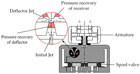
Figure 1.
Stages of flow in hydraulic amplifier of DJV.
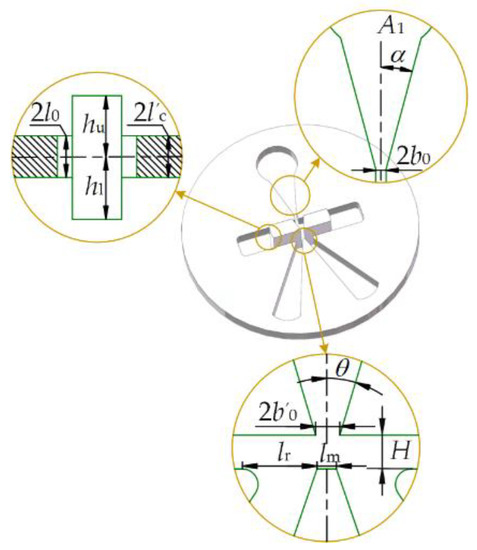
Figure 2.
Parameters of deflector jet mechanism for three-dimensional description.

Table 1.
Dimensions of deflector jet structure.
3. Methodology of Modeling Hydraulic Amplifier
3.1. Initial Jet
Before the formation of the initial jet, the fluid flows through a convergent rectangular channel. Then, the initial jet velocity can be governed by the following equations [26].
where is the average velocity at the initial jet orifice (Figure 3), is the supply pressure of hydraulic oil, is the pressure outside the orifice (back pressure), is the loss of the gradual contracting flow, and is the local loss coefficient with Equation (3) [26].
where is the frictional coefficient of the channel, given in [27] as . It follows from Equations (1)–(3) that the initial velocity .
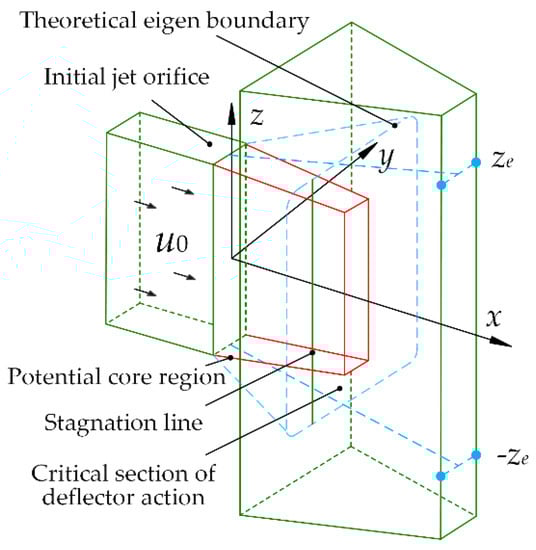
Figure 3.
Early-terminated initial jet in deflector.
Generally, the length of the potential core region for the jet can be given according to [28] as
where is the hydraulic diameter, and is the Reynolds number.
Equation (4) implies that the potential core extends far beyond the scope of the deflector, as depicted in Figure 3. However, the flow in the DJV faces a complicated situation whereby the initial jet is affected by a combination of the back pressure and the V-shaped deflector. It follows that the potential core region is terminated by recovered high pressure in the deflector. Based on an investigation into data from 3D simulation [16], some assumptions about the initial jet in the deflector are presented as follows.
Assumption 1.
The jet can be considered unaffected by the deflector before a certain perpendicular section, which is referred to as the critical section of the deflector action (the critical section for short).
Assumption 2.
The critical section is located by the stagnation line on the sidewall in the deflector. (Section 3.2).
Assumption 3.
The critical section is the interface between the initial jet and the high-pressure region in the deflector.
With the assumptions above, the two stages, the initial jet and the pressure recovery in the deflector are clearly separated by the critical section. Then, before arriving at the high-pressure region, the potential core has a varying outline along the jet direction (the x-axis in Figure 3). Based on Equation (4) and a linear assumption, the outline in an arbitrary perpendicular section at the location can be determined by
For the critical section, and , as depicted in Figure 4.
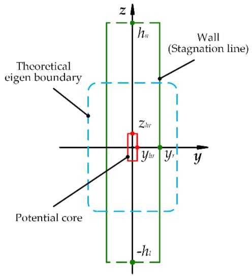
Figure 4.
Critical section of deflector action.
Assumption 4.
The flow velocity outside the potential core conforms to the Gaussian distribution, and its eigen half-width is approximately proportional to the orifice dimension in each direction.
Hence, the outside flow velocity in the section can be calculated by
in which is the velocity at the coordinates , is the dimension factor, and is the eigen half-width of the entrainment, with
where is the expansion coefficient of the theoretical eigen boundary of the jet, as illustrated in Figure 3.
For a perpendicular section , the momentum flux (momentum for short) can be calculated as
Additionally, the initial momentum at the orifice is
The conservation of momentum of the initial jet can be represented as
According to Equations (5)–(8) and (11), we can obtain a different for each , which means a nonlinear expansion of the theoretical eigen boundary. Through data fitting, the coordinate dependence of can be approximated by Equation (12) and Table 2.
Table 2.
Coefficients in Equation (12).
Hence, with Equations (5), (6), (8) and (12) substituted into Equation (7), the velocity distribution outside the potential core can be described by
Thus, the entire velocity distribution of the initial jet can be characterized as Equation (13) and the uniform velocity in the potential core. In the critical section, the velocity distribution will be the interface condition for the pressure recovery region.
3.2. Pressure Recovery in Deflector
For the jet impact acting on the sidewall of the deflector, the stagnation phenomenon always exists and divides the jet into two parts, i.e., the downstream flow and the upstream flow. Assume that the stagnation line on the sidewall is with coordinates , and , as depicted in Figure 5, which determines the location of the critical section.
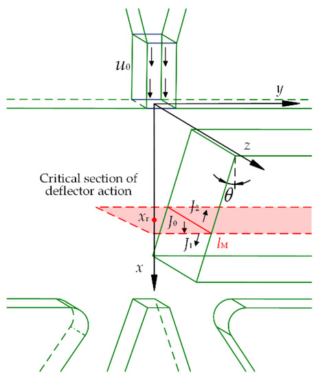
Figure 5.
Jet impact on the sidewall.
Considering that the fluid in the potential core basically keeps the same flow direction when it enters the high-pressure region, we can infer that only part of fluid collides with the sidewall.
Assumption 5.
The entrainment flow outside the potential core impacts on the sidewall, and then, flows along the sidewall, while the fluid in the potential core passes through the deflector directly without changing direction.
Therefore, according to the wall attachment model [29], the total momentum along the sidewall is
where , denoting the momentum of the downstream flow, in which is the half-width of the potential core here, calculated by Equation (5) with ; , denoting the momentum of the upstream flow; , denoting the fluid momentum outside the potential core.
According to the definition of the stagnation line , is a function of [16]; hence, Equation (14) can be solved numerically, with the result that and .
With the sidewall extruding, the kinetic energy of the fluid passing through the critical section is converted to pressure energy and a high-pressure region forms again. Because the deflector is much greater in thickness than the jet orifice, it is difficult for the fluid in the deflector far away from the jet to be affected.
Assumption 6.
The flow of the deflector outlet is limited to the extended theoretical boundary with a uniform velocity.
As depicted in Figure 3, the boundary coordinate is . Consequently, for this convergent flow, the mass continuity is expressed as
where is the deflector outlet velocity and is the critical section (Figure 4); hence,
It follows from Equations (15) and (16) that .
3.3. Deflector Jet and Pressure Recovery in Receivers
For the deflector jet, the total momentum is
However, not all fluid flowing out of the deflector is used to generate the recovery pressure of the receivers, as depicted in Figure 6. In the jet direction, the momentum acting on the shunt wedge and the two receivers can be estimated as
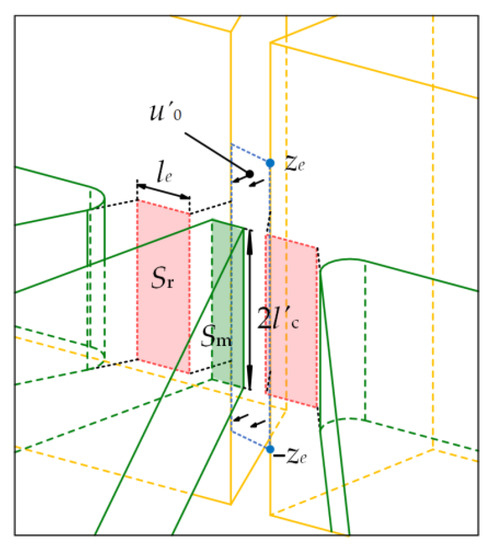
Figure 6.
Solid impact surface and effective impact area.
Simulation results [24] show that each receiver has a fluid surface to sustain the jet impact, which is referred to as the effective impact area. Approximately, the pressure in this area is uniform and equal to the pressure in the receiver.
Assumption 7.
The effective impact area is an isobaric surface with the pressure equal to the internal pressure of the receiver. The two receivers have the same effective impact area, which is fixed and unaffected by the deflectormovement.
In view of the fact that the momentum in the jet direction is zero after impact, the momentum equation in this direction can be written as
where is the solid impact surface on the shunt wedge; denotes the pressure distribution on ; and are the receiver pressures; and is the effective impact area of the receiver, decided by the effective impact width . A visual description is provided in Figure 6.
Consider the specific situation of the receiver. After impacting on the shunt wedge, the fluid flowing through the receiver obtains a large velocity component parallel to the impact surface, resulting in emergence of a low-pressure region adhering to the side of the shunt wedge, as illustrated in Figure 7. After flowing past the low-pressure region, the fluid continues to be deflected by the pressure in the receiver. Meanwhile, this deflected flow gives the closed chamber of the receiver a continuous reaction to drive the sliding spool. For a deflector jet valve, this process reflects the formation mechanism of the working pressure.
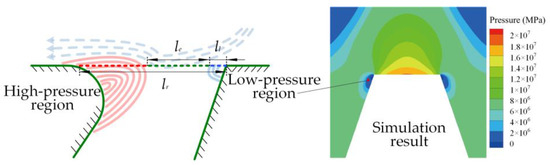
Figure 7.
Effective impact width of the receiver.
As the flow continues to deflect, the momentum in the jet direction gradually decreases to zero, and then, the flow is no longer able to provide effective momentum for the receiver. Consequently, a smooth boundary is designed to block the flow and generate a high-pressure region, which encloses the chamber of the receiver.
Thus, a low-pressure region, a high-pressure region, and a working pressure region constitute the entire pressure distribution near the receiver. Only the distance between the high-pressure region and the low-pressure region is the effective impact width (Figure 7).
This high-pressure region can be supposed to originate from another jet impact, which comes into being just outside the shunt wedge and the low-pressure region. Experimental data [30] show that when a jet travels past half of the total distance between the jet origin and the impact wall, the pressure along the jet axis will rise significantly, meaning that the jet reaches the high-pressure region. It follows that the effective impact length can be calculated as
where is the width of the low-pressure region and is the total width of the receiver opening.
With reference to the numerical simulation results (Figure 7), the width of the low-pressure region is approximately constant, with a value 0.02 mm. Then, it is learned from Equation (20) that = 0.16 mm, and has an area of 0.085 mm2.
Consider the situation of the shunt wedge. Assume that the pressure on the solid impact surface conforms to the Gaussian distribution as follows.
where is the pressure at the stagnation point on the shunt wedge, is the eigen half-width, is the distribution coefficient, and is the dimension factor.
Since the jet thickness is much greater than the width of the deflector jet, it follows that the attenuation of the impact pressure along the z-axis can be ignored. Hence, Equation (21) can be simplified as follows.
where the eigen half-width depends on specific jet scenarios. A high-speed jet formed at the deflector outlet impacts on the shunt wedge and the fluid surface of the receivers, and simulation results [16] indicate that the high-pressure region is mainly distributed on the shunt wedge. Thus, we approximately take half of the shunt wedge width as , and it can be ascertained that
Consider the outlet pressure of the deflector . According to simulations, this pressure is quite sensitive to the deflector jet distance . A fitting relationship is determined between and based on the simulation data of deflector outlet pressure at different jet distances, which can be approximately expressed by
where the units of and are Pa and meter, respectively. With the deflector outlet very close to the shunt wedge, it can be assumed that the kinetic energy of the fluid at the center of the outlet is all converted into pressure energy. With consideration of the back pressure, the pressure of the stagnation point can be computed as follows according to the Bernoulli equation.
with the result . Therefore, the pressure distribution on the solid impact surface can be determined by Equation (22), depicted in Figure 8. It is noteworthy that this distribution is effective only for the shunt wedge surface. Outside the shunt wedge is the effective impact area of the receiver, and its pressure is described by Assumption 7.
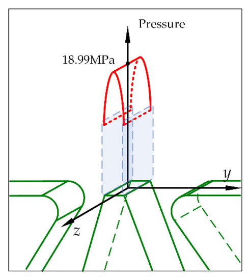
Figure 8.
Pressure distribution on the solid impact surface.
Assumption 8.
On both sides of the stagnation point, the same amount of momentum in the jet direction is depleted by the shunt wedge and the receivers; that is, each side is faced with half of the total momentum of the deflector jet.
Hence, Equation (19) is rewritten to compute the pressures in the receivers as follows.
where and are the solid impact surfaces on both sides of the stagnation point, which are determined by the deflector displacement , as depicted in Figure 9. When , it can be learned that , which is called the balance pressure; that is,
where is exactly half the solid impact surface.
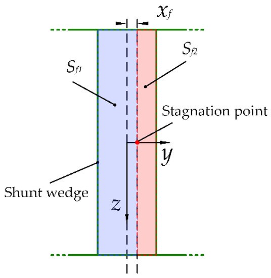
Figure 9.
Solid impact surfaces on the shunt wedge.
Further, the average pressure gain of the pilot valve of the DJV is
According to our theoretical calculations, a three-dimensional mathematical model of DJV considering the nonlinear expansion of the jet’s external boundary is constructed. Additionally, the relationship between the balance pressure and the deflector displacement can be obtained based on the model.
4. Methodology of Model Validation: Simulation and Experiment
Since the internal mechanism of the DJV’s hydraulic amplifier has been detailed by the three-dimensional theoretical model above, numerical simulations and experiments were conducted to verify its validity.
4.1. Numerical Simulation
In view of the hydraulic amplifier having a tiny structure, it is difficult to measure the flow information directly. Hence, a numerical model has been built as depicted in Figure 10. Additionally, the boundary conditions of the numerical simulation model are mainly comprised of a pressure inlet, pressure outlet and walls. Specifically, an inlet pressure of 21 MPa and an outlet pressure of 3.1 MPa are specified, which are the same as in actual scenarios. All the other surfaces are defined as non-slip wall boundaries, and it is assumed that the hydraulic oil is a Newtonian fluid with a density of 850 kg/m3 and viscosity of 0.017336 Pa·s. The Large Leddy Simulation (LES), which is supposed to be more accurate for reproducing time-varying turbulence, is applied in this case. Firstly, the RNG k-ε is used to perform the time-average numerical calculation with time steps of 1000, and then, the time-average calculation results are used as initial conditions for LES with a time step size of 0.00001 s and time steps of 2000. With the hypotheses of incompressible flow assumed, the finite volume commercial code ANSYS/FLUENT is used to solve continuity and unsteady momentum equations. Additionally, a bounded central-differencing spatial discretization scheme is employed.
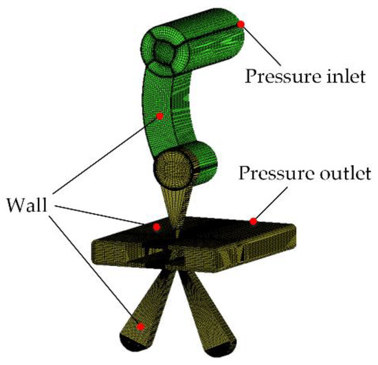
Figure 10.
Numerical model of the hydraulic amplifier.
In order to ensure the accuracy of the numerical simulation, a grid dependency test is necessary. Detailed information on five grids’ generation schemes is shown in Table 3.
Table 3.
Information on the grid schemes.
The numerical simulation results obtained by using different grid schemes are depicted in Figure 11. The simulation results denote the outlet flow rate of different grid schemes at a given time. It can be seen that the mass flow rate error is acceptable between the results using grid 4 and grid 5. In order to save on numerical time and computing cost, grid 4 is used to complete further numerical simulation. Additionally, the simulation results in the paper are obtained by solving this numerical model.
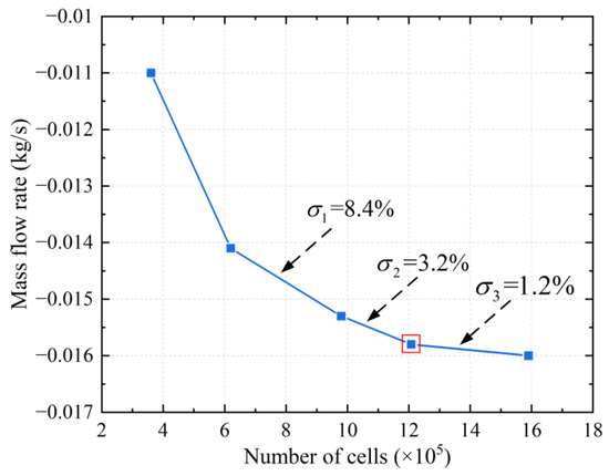
Figure 11.
Outlet mass flow rate of different grid schemes.
4.2. Experimental Method
Due to the limitations of numerical simulation, an experiment exploring the correlation between the deflector movement and the receiver pressure is carried out.
Removing the permanent magnet, the coils, and the upper pole piece of the torque motor, we can directly push the armature to move; a dial indicator is utilized to detect the displacement of the other end of the armature with a measurement precision of 0.001 mm, as depicted in Figure 12. At the same time, the armature drives the deflector to move. In this situation, the displacement proportion of the armature end to the deflector is approximately 19/12, which means the tiny movement of the deflector can be obtained indirectly. Meanwhile, with an inlet pressure given, the pressure variations in the two receivers can be detected. Two pressure sensors are installed at the bottom of the two receivers. Overall, we can obtain the pressure of two receivers under different displacements of the deflector. The practical experiment operation is represented in Figure 13.
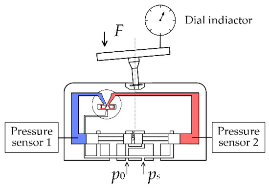
Figure 12.
Devices and experimental method.
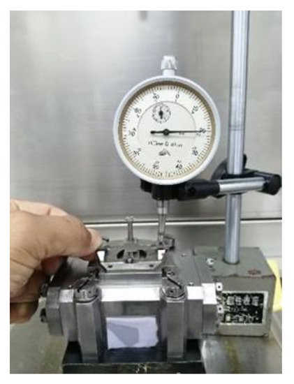
Figure 13.
Experiment operation.
5. Results of Model Validation
5.1. Description of Internal Flow Distribution
As noted above, due to the tiny structure of the hydraulic amplifier, compared with experiments, the numerical method is a more effective and realizable method to obtain the internal flow information. Based on the three-dimensional numerical model, the velocity distribution inside the deflector is verified. The velocity distributions in the deflector can be calculated according to Equation (7), with the relevant simulation results displayed in Figure 14.
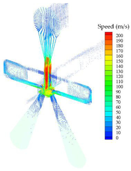
Figure 14.
Velocity distribution in the mean section.
Compare the velocity distributions of theoretical calculation and the simulation at four locations in the deflector (Figure 15). Overall, the calculation remains consistent with the data extracted from the simulation, as depicted in Figure 16. Yet, the theoretical potential core is wider; this results from Equation (4), the formula of the potential core length, not being absolutely accurate in this situation, since the initial jet velocity is relatively susceptible to the wall friction at such a high flow rate and is not uniform in practice [16].
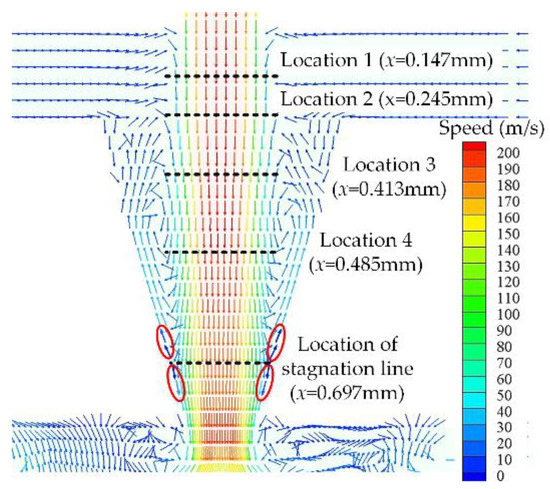
Figure 15.
Locations for comparisons in the mean section of the deflector.
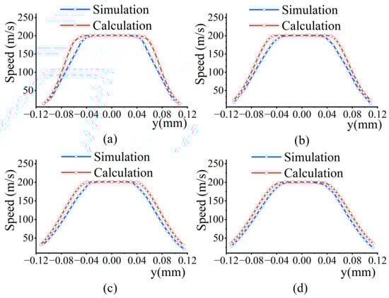
Figure 16.
Comparisons of velocity distributions in deflector. (a) x = 0.147 mm. (b) x = 0.245 mm. (c) x = 0.413 mm. (d) x = 0.485 mm.
Meanwhile, the location of the stagnation line in the simulation is measured in Figure 14. The comparison made in Table 4 shows that the theoretical model can give an accurate location of the stagnation line. It means that the model can properly reflect the flow pattern in the deflector and explain the mechanism of stagnation forming.
Table 4.
Comparison of stagnation line locations.
As regards the deflector jet, a comparative study of the impact pressure on the shunt wedge is carried out in this research. As represented in Figure 17, the overall consistency of the calculation and the simulation is available; however, influenced by the receiver opening, the simulation curve is deformed at the edge of the shunt wedge.
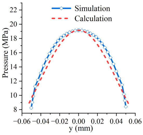
Figure 17.
Comparison of impact pressures on the shunt wedge.
5.2. Pressures in Receivers
With the actual parameters substituted, the pressures of the two receivers were calculated, with the results recorded in Appendix A. Additionally, the corresponding experimental data are listed in Appendix B.
A graphical comparison, as illustrated in Figure 18, shows that the theoretical calculation conforms to the experiment fairly well, except for an abnormal pressure deviation in the right receiver when a large deflector displacement is exerted, which is presumed to be caused by asymmetry of machining. Additionally, Figure 19 reflects the calculation performance of the theoretical model in terms of the pressure differential driving the spool valve. In addition, we compare our pressure differential results with the simulations of Jiang (2016) [31] and the experimental data of Li et al. (2021) [32]. However, since they do not take account of the outlet pressure, the pressure differential simulation results are lower. The agreement between our theoretical calculation and experimental results is satisfactory. Consider the calculation accuracy of the model, as shown in Figure 20. Except for the abnormal point, the calculation error fluctuates in a small range for both the pressures and the pressure differential. The errors are derived from the phenomenon whereby the pressure gradient of each receiver fluctuates slightly and irregularly as the deflector moves; that is, some tiny unknown factors are functioning in the actual hydraulic amplifier.
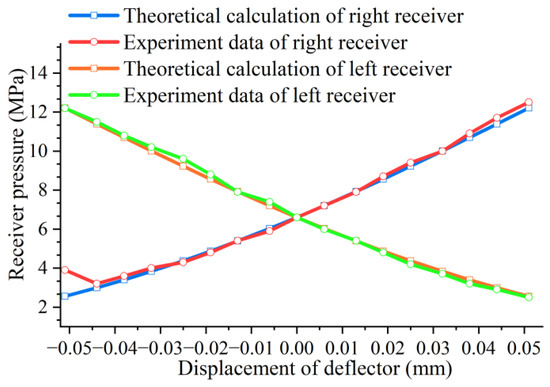
Figure 18.
Comparison of receiver pressures.
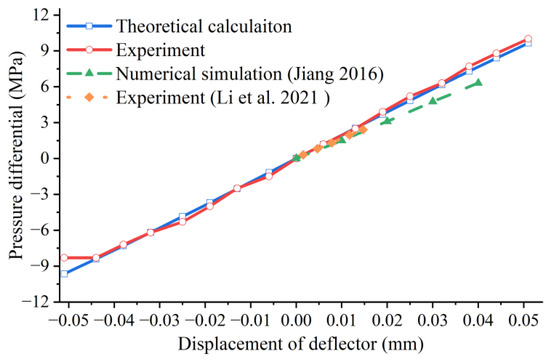
Figure 19.
Comparison of pressure differential [31,32].
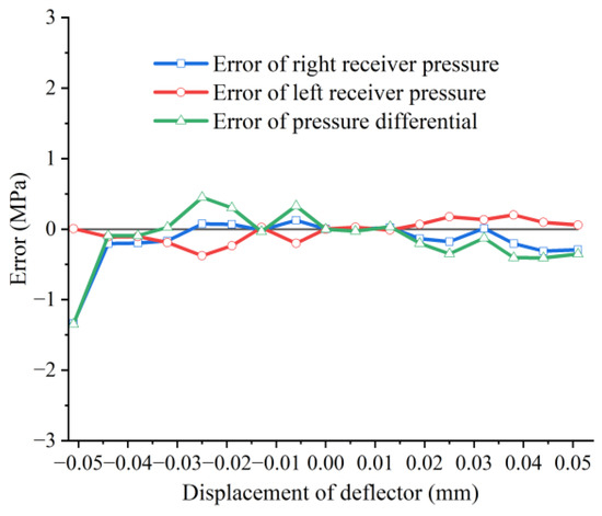
Figure 20.
Calculation errors of pressures.
Still, the validity of the theoretical model has been materially proven; hence research on the DJV can be furthered based on it.
6. Further Analysis and Discussion
Consider an actual scenario of DJV application. Due to installation and machining errors, the relative location of the deflector and the width of the shunt wedge may deviate from the design values.
A flow chart of DJV three-dimensional mathematical model establishment and uncertainty analysis of pressure indices is shown in Figure 21. The flow field characteristics of the DJV can be calculated according to the mathematical model, as we described above. Additionally, the relationship between the deflector displacement and the pressure of the two receivers can be obtained. Thus, the uncertainty of pressure indices is analyzed based on the calculation results.
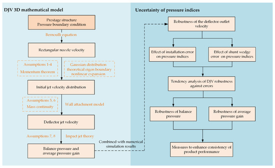
Figure 21.
Flow charts of DJV three-dimensional mathematical model establishment and uncertainty analysis of pressure indices.
6.1. Robustness of the Deflector Outlet Velocity
According to the calculation and the simulation, it can be found that the deflector outlet velocity has extraordinary robustness against location deviations of the deflector. Considering the installation error of the deflector, we can express the actual deflector jet distance as
where is the design value and is the error derived from installation. Our calculations show that when varies within a range of −5 μm to 5 μm, the fluctuation of the deflector outlet velocity is less than 0.16%, as shown in Table 5. Moreover, it follows from the numerical simulation that the deflector displacement also has very little effect on its outlet velocity.
Table 5.
Installation error dependence of the deflector outlet velocity.
Consequently, the deflector can supply a fairly stable jet for the receivers and the shunt wedge. However, the balance pressure and the pressure gain are much more sensitive to installation and machining errors.
6.2. Effect of Installation Error on Pressure Indices
According to the discussion above, it can be assumed that the deflector outlet velocity is constant. Then, from Equations (23), (24), (27) and (29) we can obtain the balance pressure , as a function of the installation error .
As depicted in Figure 22, the installation error of the deflector has little effect on pressure. For an error from −5 μm to 5 μm, the balance pressure rises by 0.08 MPa (1.2% of the standard value), which is one of the reasons that the same valves often have different balance pressures.
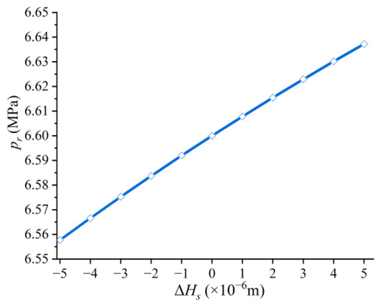
Figure 22.
Installation error dependence of balance pressure.
According to Equations (23)–(26), (28) and (29), the average pressure gain can be expressed by
For different deflector displacements, the installation error dependence of the average pressure gain is depicted in Figure 23.
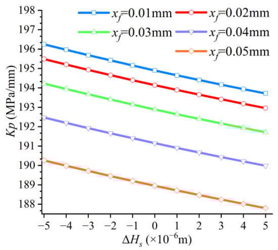
Figure 23.
Drift of average pressure gain caused by installation error.
Our calculation shows when the installation error ranges from −5 μm to 5 μm, the pressure gain of the hydraulic amplifier drops by 2.5 MPa/mm (1.3%), and the influence is approximately linear. Additionally, the average pressure gains for different deflector displacements have a consistent tendency. In any case, such a deviation of the pressure gain will not significantly affect the dynamic performance of the valve.
6.3. Effect of Shunt Wedge Error
The width error of the shunt wedge may stem from machining and erosion wear, resulting in the actual width being expressed as
where is the design value, and is the width error.
The deviation of will affect , , and in Equations (25)–(27); hence the balance pressure can be expressed as a function of .
This is represented in Figure 24.
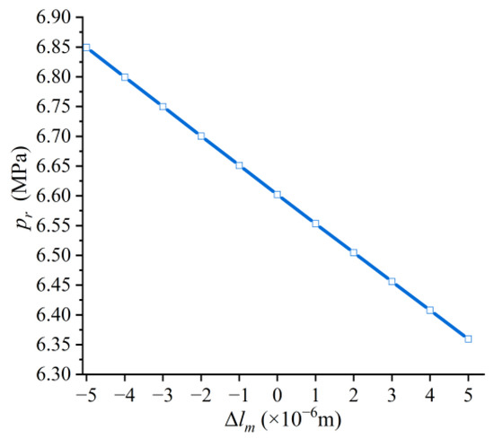
Figure 24.
Shunt wedge error dependence of balance pressure.
Therefore, the shunt wedge width has an approximately linear effect on the balance pressure. When the width error ranges from −5 μm to 5 μm, the balance pressure drops by 0.49 MPa (7.4%). By contrast, the deviation originating from the shunt wedge width error is remarkable. Hence, it is considered to be the main reason that the same valves differ in balance pressure.
From Equations (25), (26), (28) and (32), the pressure gain can be calculated by
For different deflector displacements, the correlation between the shunt wedge width error and the average pressure gain is depicted in Figure 25.
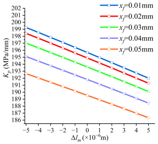
Figure 25.
Drift of average pressure gain caused by shunt wedge width variation.
Our calculation shows that when the error of the shunt wedge width ranges from −5 μm to 5 μm, the pressure gain of the hydraulic amplifier drops by 6.93 MPa/mm (3.6%), hence exerting a greater influence on the dynamic performance than the installation error.
6.4. Tendency Analysis of DJV Robustness against Errors
Since the production of servo valves often encounters the problem of performance inconsistency, it is essential to explore the mechanism of this phenomenon.
6.4.1. Robustness of Balance Pressure
It follows from Equation (30) that the derivative of the balance pressure to the installation error is
which is taken as a susceptibility index to evaluate the balance pressure robustness against the installation error, with its tendency displayed in Figure 26.
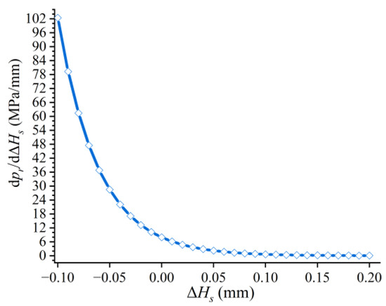
Figure 26.
Balance pressure robustness against the deflector installation error.
Therefore, when the deflector approaches the shunt wedge by 0.1 mm, the balance pressure susceptibility, when compared with that for the standard deflector installation , increases about 12 times. Conversely, if the deflector is further than the design location, the susceptibility will drop slightly. This result shows that a positive error of the jet distance is acceptable, while negative errors will lead to serious inconsistency of product pressures, namely, a plummet in the balance pressure robustness.
Consider the derivative of Equation (33) to the shunt wedge width error,
which represents the balance pressure robustness against the width error of the shunt wedge, as illustrated in Figure 27.
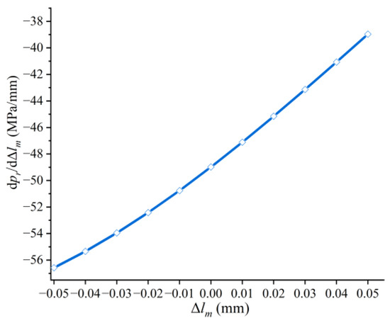
Figure 27.
Balance pressure robustness against width error of shunt wedge.
In comparison to the installation error , the shunt wedge error has a larger but more gradual effect on the balance pressure robustness. Taking both Figure 26 and Figure 27 into consideration, it can be concluded that as long as the deflector is not too close to the shunt wedge, the shunt wedge error will dominate the balance pressure fluctuation.
6.4.2. Robustness of Average Pressure Gain
According to Equation (31), the robustness tendency of the average pressure gain can be described by
As depicted in Figure 28, supposing that the deflector approaches the shunt wedge by 0.1 mm from the standard installation location, the pressure gain susceptibility will increase over 10 times. However, the opposite offset of the deflector has relatively little effect on the pressure gain robustness. Therefore, to stabilize the pressure gain of products or make them robust, the error of the jet distance should also be kept positive.
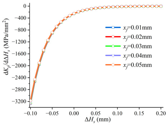
Figure 28.
Pressure gain robustness against deflector installation error.
Consider the pressure gain robustness against the shunt wedge width. The derivative of Equation (34) can be expressed by
which is illustrated in Figure 29 for different deflector displacements.
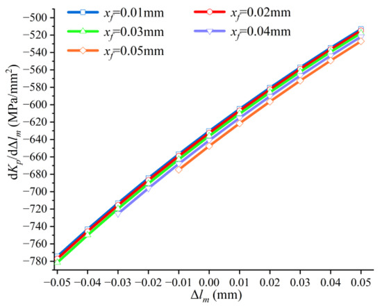
Figure 29.
Pressure gain robustness against width error of shunt wedge.
Similarly, the shunt wedge error has a much more gradual effect on the pressure gain robustness than the deflector installation error. However, from Figure 28 and Figure 29, it can be learned that when the deflector is not too close to the shunt wedge, the shunt wedge error dominates the pressure gain variation.
6.4.3. Measures to Enhance Consistency of Product Performance
The theoretical model has provided quantitative information for drifts of the DJV pressure indices and predictions about robustness tendency. The above analyses show that to avoid the inconsistency issues of servo valve products, the machining accuracy of the shunt wedge is worthy of more concern and a non-negative error of the deflector jet distance should be ensured.
Specifically, a less than 1% fluctuation of the balance pressure can be expected if the width error of the shunt wedge is limited between −0.6 μm and 0.6 μm. Additionally, the design value of the deflector jet distance can be moderately increased to improve the robustness of the pressure indices.
7. Conclusions
In view of the complexity of the deflector jet valve, the assumptions connecting the fundamental jet theory with the actual valve structure are quite essential. They provide a framework for applications of specific theorems and determine the effective scopes of diverse formulas and the interface parameters for formula switching. To a considerable extent, these assumptions are confirmed by numerical simulation and experiments. Therefore, the theoretical model based on them can provide a distinct and logical description of the flow pattern in the deflector jet valve. Furthermore, the static pressure performance of the deflector servo valve can be studied theoretically based on our three-dimensional mathematical model.
The uncertainty of the pressure indices of servo valve products, a common problem in actual scenarios, can originate from the installation error of the deflector and the machining error of the shunt wedge. For the balance pressure—the receiver pressure with the deflector centered—the two error sources, within a range of 10 microns, can bring about 1.2% and 7.4% fluctuations, respectively. Additionally, for the pressure gain, the induced fluctuations can reach 1.3% and 3.6%, respectively. That is, the error of the shunt wedge width can result in remarkable performance variation, especially for the balance pressure.
It is discovered that the deflector approaching the shunt wedge leads to rapid deterioration of performance robustness against errors, which can magnify the inconsistency of the pressure indices of servo valves. However, as long as the deflector is not too close to the shunt wedge, the performance fluctuation will be dictated by the width error of the shunt wedge. Hence, in the actual production of servo valves, the machining accuracy of the shunt wedge and non-negative errors of the deflector jet distance should both be guaranteed to achieve more stable product performance. Specifically, the width error of the shunt wedge should be limited between −0.6 μm and 0.6 μm to guarantee that the fluctuation of the balance pressure is less than 1%.
Author Contributions
Conceptualization, Y.R. and H.Y.; methodology, H.Y. and Y.R.; validation, Q.M. and H.H.; formal analysis, Y.R. and Q.M.; investigation, Y.R. and H.Y.; resources, Z.Z.; writing—original draft preparation, H.Y., Q.M. and Y.R. All authors have read and agreed to the published version of the manuscript.
Funding
This research was funded by the National Natural Science Foundation of China (grant number 51775032) and the Foundation of the Key Laboratory of Vehicle Advanced Manufacturing, Measuring and Control Technology, Beijing Jiaotong University, Ministry of Education, China.
Institutional Review Board Statement
Not applicable.
Informed Consent Statement
Not applicable.
Data Availability Statement
The data will be made available from the corresponding author upon reasonable request.
Conflicts of Interest
The authors declare no conflict of interest.
Appendix A
Table A1.
Calculations of receiver pressures.
Table A1.
Calculations of receiver pressures.
| Displacement/mm | Pressure of Left Receiver/MPa | Pressure of Right Receiver/MPa |
|---|---|---|
| −0.051 | 11.87 | 2.56 |
| −0.044 | 11.11 | 3.02 |
| −0.038 | 10.47 | 3.44 |
| −0.032 | 9.83 | 3.88 |
| −0.025 | 9.09 | 4.43 |
| −0.019 | 8.48 | 4.92 |
| −0.013 | 7.87 | 5.43 |
| −0.006 | 7.18 | 6.06 |
| 0 | 6.61 | 6.61 |
| 0.006 | 6.06 | 7.24 |
| 0.013 | 5.43 | 8.05 |
| 0.019 | 4.92 | 8.83 |
| 0.025 | 4.43 | 9.68 |
| 0.032 | 3.88 | 9.83 |
| 0.038 | 3.44 | 10.47 |
| 0.044 | 3.02 | 11.11 |
| 0.051 | 2.56 | 11.87 |
Appendix B
Table A2.
Experimental data on receiver pressures.
Table A2.
Experimental data on receiver pressures.
| Displacement/mm | Pressure of Left Receiver/MPa | Pressure of Right Receiver/MPa |
|---|---|---|
| −0.051 | 12.2 | 3.9 |
| −0.044 | 11.5 | 3.2 |
| −0.038 | 10.8 | 3.6 |
| −0.032 | 10.2 | 4.0 |
| −0.025 | 9.6 | 4.3 |
| −0.019 | 8.8 | 4.8 |
| −0.013 | 7.9 | 5.4 |
| −0.006 | 7.4 | 5.9 |
| 0 | 6.6 | 6.6 |
| 0.006 | 6.0 | 7.2 |
| 0.013 | 5.4 | 7.9 |
| 0.019 | 4.8 | 8.7 |
| 0.025 | 4.2 | 9.4 |
| 0.032 | 3.7 | 10 |
| 0.038 | 3.2 | 10.9 |
| 0.044 | 2.9 | 11.7 |
| 0.051 | 2.5 | 12.5 |
References
- Tamburrano, P.; Plummer, A.R.; Distaso, E.; Amirante, R. A review of electro-hydraulic servovalve research and development. Int. J. Fluid Power 2018, 20, 53–98. [Google Scholar] [CrossRef]
- Somashekhar, S.H.; Singaperumal, M.; Kumar, R.K. Modelling the steady-state analysis of a jet pipe electrohydraulic servo valve. Proc. Inst. Mech. Eng. Part I J. Syst. Control Eng. 2006, 220, 109–129. [Google Scholar] [CrossRef]
- Somashekhar, S.H.; Singaperumal, M.; Kumar, R.K. Mathematical modelling and simulation of a jet pipe electrohydraulic flow control servo valve. Proc. Inst. Mech. Eng. Part I J. Syst. Control Eng. 2007, 221, 365–382. [Google Scholar] [CrossRef]
- Pham, X.H.S. Effects of surface roughness and fluid on amplifier of jet pipe servo valve. Int. J. Eng. Sci. (IJES) 2016, 5, 11–23. [Google Scholar]
- Li, Y. Mathematical modelling and characteristics of the pilot valve applied to a jet-pipe/deflector-jet servovalve. Sens. Actuators A Phys. 2016, 245, 150–159. [Google Scholar] [CrossRef]
- Wang, X.H.; Li, Z.J.; Sun, S.W.; Zheng, G. Investigation on the Prestage of a Water Hydraulic Jet Pipe Servo Valve Based on CFD. Appl. Mech. Mater. 2012, 197, 144–148. [Google Scholar] [CrossRef]
- Yin, Y.; Wang, Y. Pressure characterization of the pre-stage of jet pipe servo valve. J. Aerosp. Power 2015, 30, 3058–3064. [Google Scholar]
- Chu, Y.; Yuan, Z.; He, X.; Dong, Z. Model Construction and Performance Degradation Characteristics of a Deflector Jet Pressure Servo Valve under the Condition of Oil Contamination. Int. J. Aerosp. Eng. 2021, 2021, 8840084. [Google Scholar] [CrossRef]
- Zhu, Y.; Li, Y. Development of a deflector-jet electrohydraulic servovalve using a giant magnetostrictive material. Smart Mater. Struct. 2014, 23, 115001. [Google Scholar] [CrossRef]
- Dhinesh, K.S. Fluid Metering Using Active Materials. Ph.D. Thesis, University of Bath, Bath, UK, 2011. [Google Scholar]
- Shang, Y.; Zhang, X.; Hu, C. Optimal design for amplifier of jet deflector servo valve. Mach. Tool Hydraul. 2015, 43, 11–15. [Google Scholar]
- Zhao, K. Jet Pipe Servo Valve Flow Modeling and Characteristic Research. Master’s Thesis, Wuhan University of Science and Technology, Wuhan, China, 2015. [Google Scholar]
- Yang, Y. Analysis and Experimental Research of pre-Stage Jet Flow Field in Hydraulic Servo Valve. Master’s Thesis, Harbin Institute of Technology, Harbin, China, 2006. [Google Scholar]
- Jiang, D.; Xu, M. Simulation based on Fluent for pre-stage of deflector jet servo valve. Chin. Hydraul. Pneum. 2016, 6, 48–53. [Google Scholar]
- Yin, Y.; Zhang, P.; Cen, B. Pre-stage flow field analysis on deflector jet servo valves. Chin. J. Constr. Machi. 2015, 13, 1–7. [Google Scholar]
- Yan, H.; Ren, Y.; Yao, L.; Dong, L. Analysis of the Internal Characteristics of a Deflector Jet Servo Valve. Chin. J. Mech. Eng. 2019, 32, 31. [Google Scholar] [CrossRef]
- Saha, B.K.; Peng, J.; Li, S. Numerical and Experimental Investigations of Cavitation Phenomena Inside the Pilot Stage of the Deflector Jet Servo-Valve. IEEE Access 2020, 8, 64238–64249. [Google Scholar] [CrossRef]
- Wang, C.; Ding, F.; Li, Q.; Xu, X. Dynamic characteristics of electro-hydraulic position system controlled by jet-pan servovalve. J. Chongqing Univ. 2003, 26, 11–15. [Google Scholar]
- Yin, Y.; Zhang, P.; Zhang, Y. Research on pressure characteristic of deflector jet servo valve. Fluid Power Transm. Control 2014, 65, 10–15. [Google Scholar]
- Chen, J.; Li, F.; Yang, Y.; Gao, Y. Mathematical Modelling and Hierarchical Encourage Particle Swarm Optimization Genetic Algorithm for Jet Pipe Servo Valve. Comput. Intell. Neurosci. 2022, 2022, 9155248. [Google Scholar] [CrossRef]
- Sangiah, D.K.; Plummer, A.R.; Bowen, C.R.; Guerrier, P. A novel piezohydraulic aerospace servovalve. Part 1: Design and modelling. Proc. Inst. Mech. Eng. Part I J. Syst. Control Eng. 2013, 227, 371–389. [Google Scholar]
- Yan, H.; Wang, F.-J.; Li, C.-C.; Huang, J. Research on the jet characteristics of the deflector–jet mechanism of the servo valve. Chin. Phys. B 2017, 26, 44701. [Google Scholar] [CrossRef]
- Yan, H.; Bai, L.; Kang, S.; Dong, L.; Li, C. Theoretical model and characteristics analysis of deflector-jet servo valve’s pilot stage. J. Vibroeng. 2017, 19, 4655–4670. [Google Scholar] [CrossRef]
- Yan, H.; Mao, Q.; Ren, Y.; Yao, L. Mechanism analysis of the secondary jet of jet deflector servo valve. In Proceedings of the 2019 IEEE 8th International Conference on Fluid Power and Mechatronics, Wuhan, China, 10 April 2019. [Google Scholar]
- Saha, B.K.; Li, S.; Lv, X. Analysis of Pressure Characteristics under Laminar and turbulent flow states inside the pilot stage of a deflection flapper servo-valve: Mathematical modeling with CFD study and experimental validation. Chin. J. Aeronaut. 2020, 33, 1107–1118. [Google Scholar] [CrossRef]
- Japan Society of Mechanical Engineering (JSME). Fluid Mechanics; Peking University Press: Beijing, China, 2013. [Google Scholar]
- Technical Centre for Process System Design. Technical Regulation for Systems Engineering Design HG/T 20570.7-95; Ministry of Chemical Industry of the People’s Republic of China: Beijing, China, 1996; pp. 14–57.
- Harsha, P.T. Free Turbulent Mixing: A Critical Evaluation of Theory and Experiment; Arnold Engineering Development Center, Air Force Systems Command, United States Air Force: Arnold Air Force Base, TN, USA, 1971; pp. 13–75.
- Bourque, C.; Newman, B.G. Reattachment of a Two-Dimensional, Incompressible Jet to an Adjacent Flat Plate. Aeronaut. Q. 1960, 11, 201–232. [Google Scholar] [CrossRef]
- Dong, Z. Jet Mechanics; Science Press: Beijing, China, 2005; pp. 49–62. [Google Scholar]
- Jiang, D. Pre-Stage Flow Field Simulation and Dynamic Characteristics of Deflector Jet Servo Valve. Master’s Thesis, Jiangsu University, Jiangsu, China, 2016. [Google Scholar]
- Li, S.; Yin, Y.; Yuan, J.; Guo, S. Analysis of Three-Dimensional Flow Field Inside the Pilot Stage of the Deflector Jet Servo Valve. Preprint, 2021. [Google Scholar] [CrossRef]
Publisher’s Note: MDPI stays neutral with regard to jurisdictional claims in published maps and institutional affiliations. |
© 2022 by the authors. Licensee MDPI, Basel, Switzerland. This article is an open access article distributed under the terms and conditions of the Creative Commons Attribution (CC BY) license (https://creativecommons.org/licenses/by/4.0/).