Identification of Vehicle Loads on an Orthotropic Deck Steel Box Beam Bridge Based on Optimal Combined Strain Influence Lines

Abstract

Vehicles are critical living loads to bridge structure; thus, identifying vehicle loads is very important for structural health monitoring and safety evaluations. This paper proposed a load identification method based on an optimal combined strain influence line. Firstly, two types of strain gauges were arranged at the lower edge of a deck to monitor the strain response when vehicles cross the deck. One type of sensor was installed at the lower edge of the deck between U-ribs to detect axle information, including the number of axles, wheelbase, and vehicle speed. The other type of sensor was set on the lower edge of U-ribs to identify the axle’s weight. Secondly, structural responses under the vehicle load with known weights across the bridge was used to identify the strain influence line by using least square method. Because the local mechanical characteristic of the deck was very prominent under the wheel load, the strain influence line was short and susceptible to the transverse position of the vehicle. An index of variation coefficient is proposed as the object function, and an optimal combined strain influence line was developed using a genetic algorithm to decrease the influence of the transverse position of the load. Finally, the unknown vehicle load can be identified based on a calibrated combined strain influence line. A numerical simulation and an experimental test were carried out to validate the effectiveness and anti-noise performance of the proposed method. The identified results showed that the proposed algorithm has good accuracy and anti-noise performance.

1. Introduction

With the rapid development of the economy, the volume of freight transported on roads is overgrowing, and overloading is a frequent phenomenon. The orthotropic deck steel box girder structure is widely used in large-span bridges due to the advantage of being lightweight and possessing high rigidity. Due to the prominent local force in the orthotropic deck, frequent vehicle loads often lead to fatigue damage with respect to the deck or even failure of the bridge. Some scholars research bridge safety assessment methods based on moving vehicle loads. Pisal and Jangid [1] study the effectiveness of tuned mass friction dampers in reducing undesirable resonant responses of the bridge subjected to multi-axle vehicle loads. Yu et al. [2] proposed bridge damage identification methods from moving load-induced deflection using wavelet transforms and the Lipschitz exponent. Nie et al. [3] proposed a novel damage detection approach using only two sensors to detect the damage of bridge subjected to a moving vehicle. Therefore, accurately identifying vehicle loads is crucial to the safety assessment of bridges, health monitoring, and traffic statistics [4,5,6]. Law [7] proposed a time domain method using the bending moment and acceleration measurements to identify the load history of each axle of a vehicle. Dowling et al. [8] developed a fully automated calibration procedure for moving force identifications based on the cross-entropy optimization method. Lourens et al. [9] proposed an augmented Kalman filter for moving vehicle identifications and used experiment tests to validate the accuracy of the method. Sun et al. [10] developed an inverse analysis technique based on the finite element method and mode superposition method for impact force identification. The Bridge Weigh-in-motion (B-WIM) system is a technique for monitoring and identifying vehicle loads by placing sensors (e.g., strain gauges) on the underside of bridges, which is cheap, nondestructive to the roadway, and without effects of traffic [11,12,13]. B-WIM is mainly based on the Moses [14] algorithm. It constructs an error function between the measured and theoretical strain and solves the vehicle’s axle weight and gross weight using the least square method. The precision of the actual influence line extraction affects the accuracy of the vehicle’s load identification. The practical simple support bridge is between simple support and consolidation constraints at both ends. For the usual B-WIM system, the recognition of axle information, such as speed, the number of axles, and wheelbase, is a prerequisite for axle weight identification. Chatterjee [15] proposed a wavelet-based method for detecting information on the axle. Deng [16] proposed an equivalent shear method for the identification of axle information by only using the strain response collected by weighing sensors. It does require special axle information detection devices. O’Brien et al. [17] proposed a method for detecting axle information based on shear strains. Ma et al. [18] used accelerometers to capture vehicle axle information by using a peak filter, and magnetometers were utilized to evaluate vehicle speeds by detecting changes in the magnetic field.

After axle information has been identified, the axle’s weight was predicted by minimizing the difference between measured and predicted bridge responses based on the influence theory. Znidaric [19] promoted the identification accuracy of the influence line by adjusting constraint conditions on the support and smoothing the peak of the response to match the actual bridge engineering situation. Zhang et al. [20] proposed an iterative dynamic weighing algorithm between the Morse algorithm and the measured influence line to correct the ill-condition problem of the equation. Zhao [21] followed the method proposed by Brien [22] and used influence lines calibrated by field tests to calculate axle weights. Moreover, he researches the influence of the choice of influence lines, the shape of the influence line, and the sampling frequency during the axle’s weight identification. Leng [23] proposed a maximum likelihood estimation method for obtaining the influence line of a bridge structure. The algorithm used different girder types for calibration and identification of the influence line, and it was found that the algorithm was highly noise resistant. Rowley [24] applied Tikhonov regularization to the traditional B-WIM algorithm to improve vehicle load identification accuracy. O’Brien [25] adopted the L curve criterion to obtain the optimal regularization parameter for the Moses algorithm. The research results show that the regularized recognition accuracy is significantly better than the original Moses algorithm and insensitive to road surface roughness.

The above methods are mostly used for simply supported girders, slabs, steel girders, and truss bridges, and they do not consider the influence of the transverse position of the vehicle, which is a one-dimensional B-WIM system. However, the local stress of the deck is very prominent for the orthotropic deck steel box girder structure. The variation in the transverse position of the vehicle on the bridge deck greatly influences the load’s identification due to the local force characteristic of the orthotropic deck, so it needs to locate the vehicle’s transverse position [26]. The one-dimensional B-WIM system is not suitable for this type of bridge. Quilligan [27] investigated the two-dimensional B-WIM algorithm based on the influence surface and conducted experimental studies on integral slab bridges and beam bridges, respectively. Zhao [28] proposed an improved two-dimensional B-WIM algorithm for a simply supported T-beam bridge, which considered the transverse distribution of wheel loads on each main girder and calibrated influence lines for each main girder separately in the field. The method achieved superior recognition results after a field test on a US highway. Yu et al. [29] proposed a method of identifying the transverse position, axle weight, and gross weight based on weight sensors. The method took into account the effects of road flatness, vehicle speed, vehicle width, and different measurement points on the recognition accuracy and is validated in field trails. Zhang [30] proposed a virtual monitoring method for the fatigue assessment of orthotropic steel decks. He found that using influence surfaces for identifying vehicle loads improved the recognition accuracy. The two-dimensional algorithm can take the effect of vehicle loads into account at different locations laterally. However, it requires the calibration of the influence surface of the structure, which is a troublesome problem in practical engineering, and it needs to locate the transverse position of vehicles on the bridge accurately.

This paper applied the B-WIM system to the vehicle’s load identification of an orthotropic deck steel box beam bridge. Two types of strain gauges were arranged at the lower edge of the deck to monitor structural strain response. Based on the measured strain response, the vehicle’s information, including the number of axles, the wheelbase, and vehicle speed, was identified. An optimized combined strain influence line was obtained by a genetic algorithm based on a proposed index of variable coefficient, which was insensitivity to the transverse position of the vehicle. Then, the unknown vehicle load was identified based on the calibrated combined strain influence line. Finally, a numerical simulation and an experimental test were carried out to validate the effectiveness and anti-noise performance of the proposed method.

2. Identification Methods

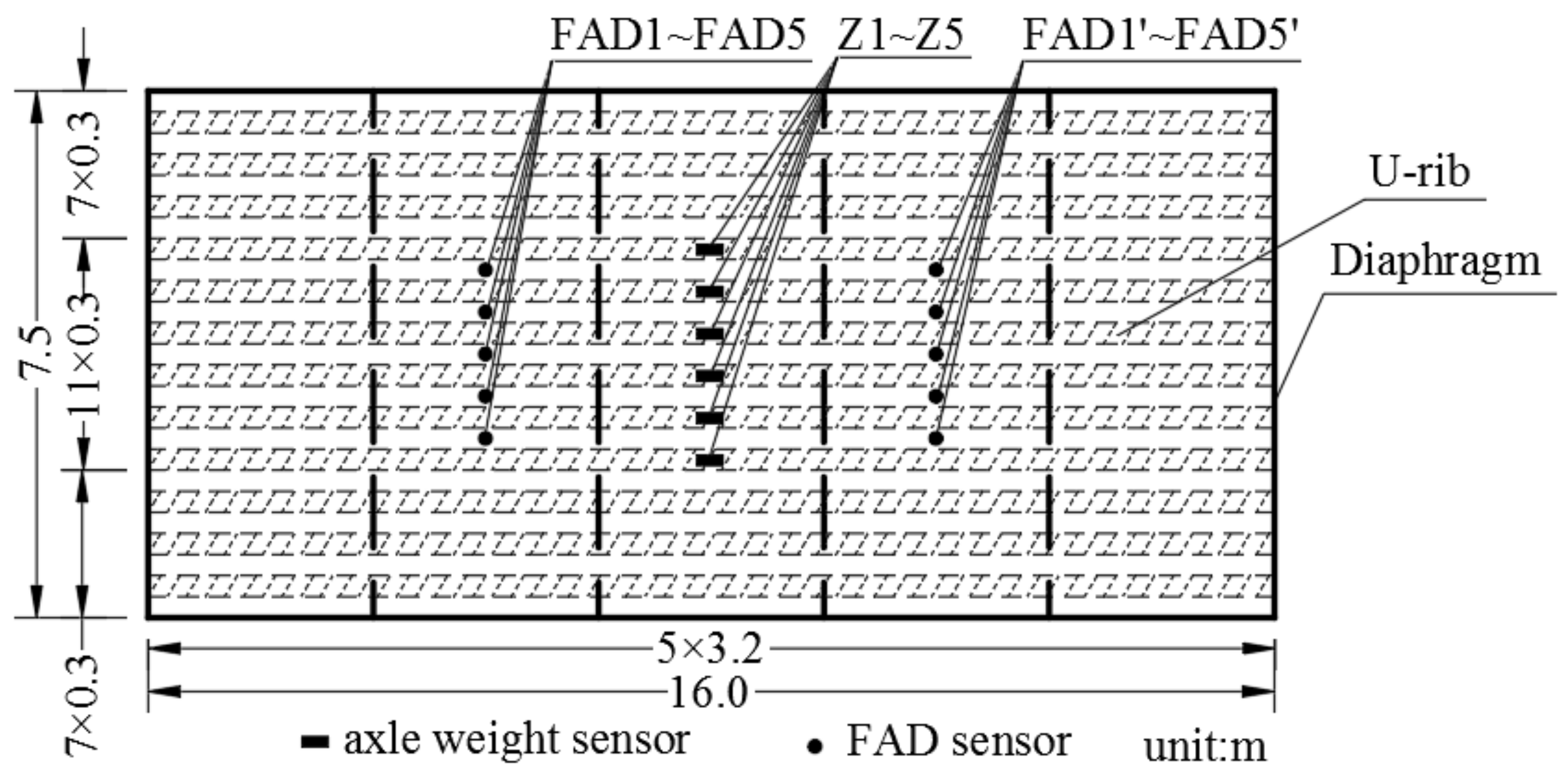
In order to identify vehicle loads on the orthotropic deck steel box beam bridge, two types of sensors need to be placed under the deck. One type is the Free-of-Axle Detector (FAD) sensor for detecting axle information such as the number of axles, wheelbase, and vehicle speed [31], which is installed at the lower edge of the deck between U-ribs. The other type of sensor is used to identify the axle’s weight and is set on the lower edge of the U-rib. The entire layout of sensor placements is shown in Figure 1.

2.1. Axle Information Recognition

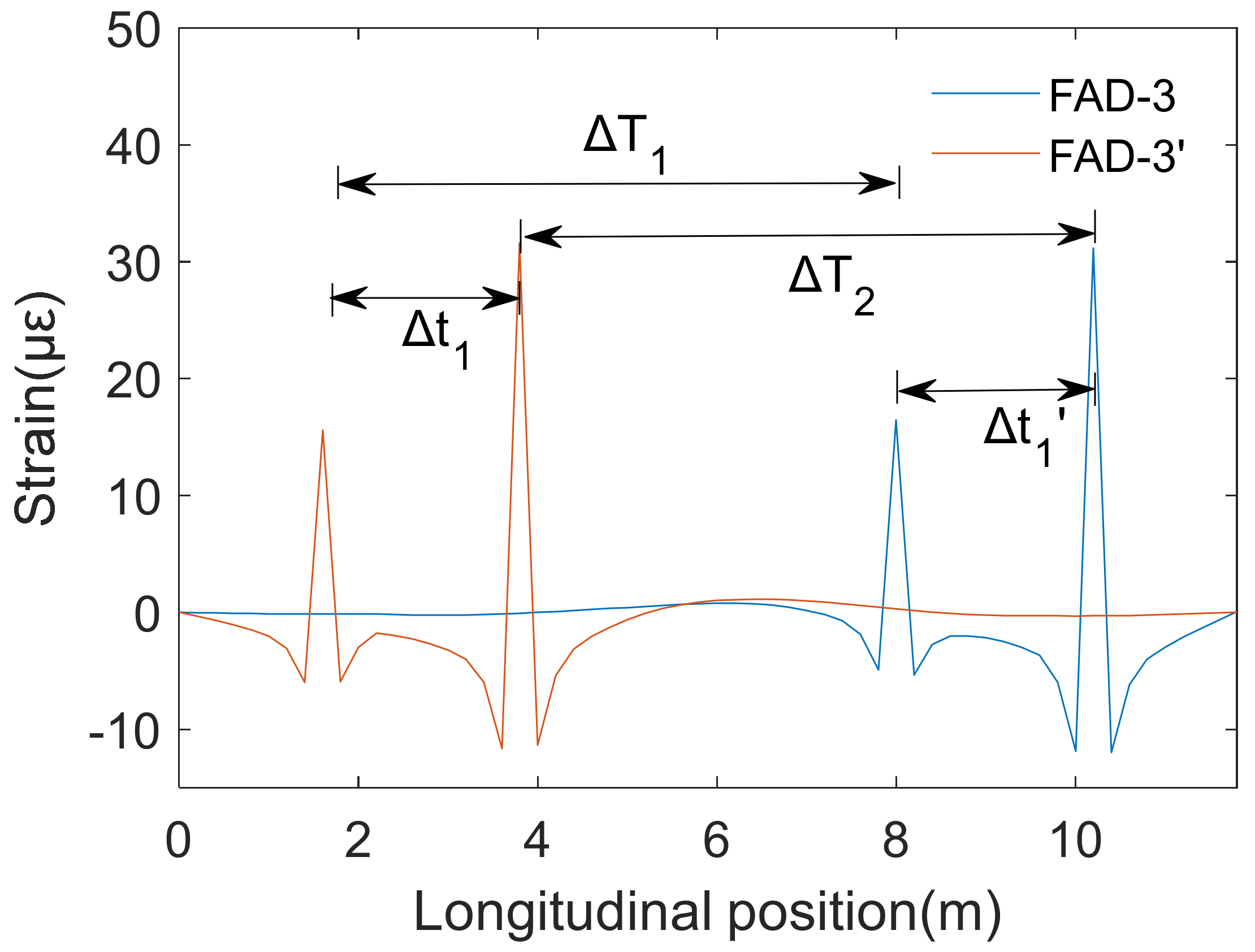
The FAD sensor identified axle information by monitoring the local response of the deck. FAD is ideally suited for detecting axle information with respect to the orthotropic deck with significant local forces and short influence lines. When the vehicle drives over the bridge, the FAD sensor will collect a significant peak response, as shown in Figure 2.

The number of peak points of the same FAD sensor represents the number of axles of the vehicle (here denoted as N_A), and the monitoring section spacing of the FAD sensor is D. The vehicle’s speed can be identified according to the time interval of the same axle driving through different sections of the FAD sensor (denoted as $\Delta \mathrm{T}$). The multi-axle monitoring results can be averaged considering the noise effect as follows.

$$v=\frac{\mathrm{D}}{\frac{1}{{\mathrm{N}}_{\mathrm{A}}}{\displaystyle \sum _{i=1}^{{\mathrm{N}}_{\mathrm{A}}}\Delta {\mathrm{T}}_i}}$$

(1)

Due to the localization of the deck force, when the wheel is far from a specific FAD sensor, the measured response is smaller, and the signal-to-noise ratio is lower, so multiple FAD sensors are deployed. The measurement point with a larger response can be selected to identify the vehicle’s speed.

By extracting time interval $\Delta t$ between adjacent peak points in the strain response measured by the same FAD sensor and multiplying it by the vehicle’s speed, we can obtain wheelbase $B_i$ (here, it is defined as the distance between the latter axle and the former axle).

$$B_i=v\times \frac{1}{2}(\Delta t_1+\Delta t_1^{\prime })$$

(2)

2.2. Strain Influence Line Identification

Next, a calibrated vehicle with a known axle weight and wheelbase information passes over the bridge deck, and the axle weight sensor collects the corresponding strain response; moreover, the strain influence line caused by the unit axle weight is identified by analyzing the strain response. Due to the local force characteristics of the orthotropic bridge deck, the strain influence line length of the measurement points on the U-rib is approximately the spacing between the front span and back span of the diaphragm [32]; thus, it can be taken as a three-span spacing of the diaphragm. The method is detailed as follows.

(1)

Assuming a calibrated vehicle, its axle weight is A_n (n = 1,2,...,N_A, N_A is the number of axles), and the wheelbase is B_n (n = 1,2,...,N_A, for uniformly descriptions, and B₁ = 0 is defined).

(2)

Assuming that the strain influence line of measurement point i to be identified is $I_i$ and the length of influence line is N_I, here, it denotes the sample point number. Take a moment when the first axle of the calibration vehicle passes the starting point of the strain influence line and define it as $t_0=0$; then, denote the starting point position as $d_0=0$. The sample frequency of signal is f, and the vehicle spacing between the two consecutive sample points is calculated as $\Delta d=\frac{v}{f}$. So at moment $t_k$ (k = 0, 1, 2,…,K, K is the number of points sampled when the last axle of the vehicle passes the end of the strain influence line), the longitudinal position of the vehicle on the bridge is $d_k=k·\Delta d$, and the strain response of measurement point i at moment $t_k$ can be expressed as follows:

$${\mathbf{\epsilon }}_i(t_k)={\mathbf{\epsilon }}_i(d_k)={\displaystyle \sum _{n=1}^{{\mathrm{N}}_{\mathrm{A}}}{A}_n{I}_i}(d_k-c_n)$$

(3)

$$c_n={\displaystyle \sum _{n=1}^{{\mathrm{N}}_{\mathrm{A}}}{B}_n}·f/v$$

(4)

where $I_i(d_k-c_n)$ is the value of the influence line for the nth axle of the calibration vehicle at position $d_k$, and $c_n$ is the difference in sampling points between the nth axle and the first axle of the calibration vehicle.

For all moments, the strain response of measurement point i can be expressed in matrix form as follows.

$${\left[A\right]}_{({\mathrm{N}}_{\mathrm{I}}+C_{\mathrm{N}}{}_{{}_{\mathrm{A}}}-1)\times {\mathrm{N}}_{\mathrm{I}}}{\left[I_i\right]}_{{\mathrm{N}}_{\mathrm{I}}\times 1}={\left[{\mathbf{\epsilon }}_i\right]}_{({\mathrm{N}}_{\mathrm{I}}+C_{\mathrm{N}}{}_{{}_{\mathrm{A}}}-1)\times 1}$$

(5)

$$\begin{array}{l}{\left[A\right]}_{({\mathrm{N}}_{\mathrm{I}}+C_{\mathrm{N}}{}_{{}_{\mathrm{A}}}-1)\times {\mathrm{N}}_{\mathrm{I}}}={\left[A_1\right]}_{({\mathrm{N}}_{\mathrm{I}}+C_{\mathrm{N}}{}_{{}_{\mathrm{A}}}-1)\times {\mathrm{N}}_{\mathrm{I}}}+{\left[A_2\right]}_{({\mathrm{N}}_{\mathrm{I}}+C_{\mathrm{N}}{}_{{}_{\mathrm{A}}}-1)\times {\mathrm{N}}_{\mathrm{I}}}+\dots +{\left[A_{{\mathrm{N}}_A}\right]}_{({\mathrm{N}}_{\mathrm{I}}+C_{\mathrm{N}}{}_{{}_{\mathrm{A}}}-1)\times {\mathrm{N}}_{\mathrm{I}}}\\ \hspace{1em}\hspace{1em}\hspace{1em}\hspace{1em}\hspace{1em}\hspace{0.33em}\hspace{0.33em}\hspace{0.17em}={\displaystyle \sum _{n=1}^{{\mathrm{N}}_{\mathrm{A}}}{\left[A_n\right]}_{({\mathrm{N}}_{\mathrm{I}}+C_{\mathrm{N}}{}_{{}_{\mathrm{A}}}-1)\times {\mathrm{N}}_{\mathrm{I}}}}\end{array}$$

(6)

$${\left[A_n\right]}_{({\mathrm{N}}_{\mathrm{I}}+C_n-1)\times {\mathrm{N}}_{\mathrm{I}}}=\left[\begin{array}{ccccc}0& 0& \dots & 0& 0\\ ⋮& ⋮& {\left[0\right]}_{(C_n-1)\times {\mathrm{N}}_{\mathrm{I}}}& ⋮& ⋮\\ 0& 0& \dots & 0& 0\\ A_n& 0& \dots & 0& 0\\ 0& A_n& \dots & 0& 0\\ ⋮& ⋮& ⋮& ⋮& ⋮\\ 0& 0& \dots & A_n& 0\\ 0& 0& \dots & 0& A_n\\ 0& 0& \dots & 0& 0\\ ⋮& ⋮& {\left[0\right]}_{(C_{{\mathrm{N}}_{\mathrm{A}}}-C_n)\times {\mathrm{N}}_{\mathrm{I}}}& ⋮& ⋮\\ 0& 0& \dots & 0& 0\end{array}\right]$$

(7)

Considering the effects of noise and vehicle vibration to the structural response, strain influence line $I_i$ can be estimated based upon the measured strain response of measurement point i using the least squares method.

$$I_i=A^{+}{\mathbf{\epsilon }}_i={(A^{\mathrm{T}}A)}^{-1}{A}^{\mathrm{T}}{\mathbf{\epsilon }}_i$$

(8)

2.3. Optimal Combined Strain Influence Line

The strain influence line can be identified separately for different measurement points. Theoretically, when the vehicle passes through the bridge in a determined transverse position, only one measurement point datum is needed during vehicle load identification using the influence line. However, when the transverse position of the vehicle changes, it is necessary to identify the influence lines of multiple transverse positions in advance. Then, the influence line corresponding to the transverse position of the vehicle load is used to identify the unknown load. Moreover, when the wheels are transversely far from the measurement point, the measured strain response is smaller, and the signal-to-noise ratio is lower. In order to facilitate the actual vehicle load’s identification, here, an optimizing analysis is carried out to find a combination of measurement point responses that is insensitive to the vehicle’s transverse position, and the optimal combined strain response is used to identify the corresponding combined strain influence line. Finally, the unknown load is identified based on the combined strain influence line. The detailed method is as follows.

Let the calibration vehicle pass over the bridge at transverse position k, we can extract the maximum strain response measured by the axle’s weight sensor. Calculate the maximum of the combined strain response at the measurement points:

$$y_j={\displaystyle \sum _{i=1}^{{\mathrm{N}}_{\mathrm{s}}}{x}_i·s_i}$$

(9)

where ${\mathrm{N}}_{\mathrm{s}}$ is the number of measurement points, $x_i$ is the combined coefficient of measurement points, and $s_i$ is the maximum value of strain response of measurement point i.

Let the vehicle pass through the bridge deck several times from different transverse positions k, we can obtain the corresponding maximum combined strain response, and then we calculate its variation coefficient according to the following Formula [14]:

$$c_v=\frac{\sigma (y_k)}{\mu (y_k)}$$

(10)

where $\sigma$ and $\mu$ is the mean and standard deviation of the maximum value of combined responses, respectively.

The smaller the variation coefficient, the less sensitive the corresponding combination strain to the transverse position of the vehicle load; thus, the optimal combination can be determined by searching for the combination with the smallest variation coefficient. The objective function to be optimized is as follows:

$$f_o(X)=c_v=\frac{\sigma ({\displaystyle \sum _{i=1}^{{\mathrm{N}}_{\mathrm{s}}}{x}_i·s_i})}{\mu ({\displaystyle \sum _{i=1}^{{\mathrm{N}}_{\mathrm{s}}}{x}_i·s_i})}$$

(11)

where $X=[x_1,x_2,\dots ,x_{{\mathrm{N}}_s}]$ denotes independent variable parameters consisting of ${\mathrm{N}}_{\mathrm{s}}$ measurement points.

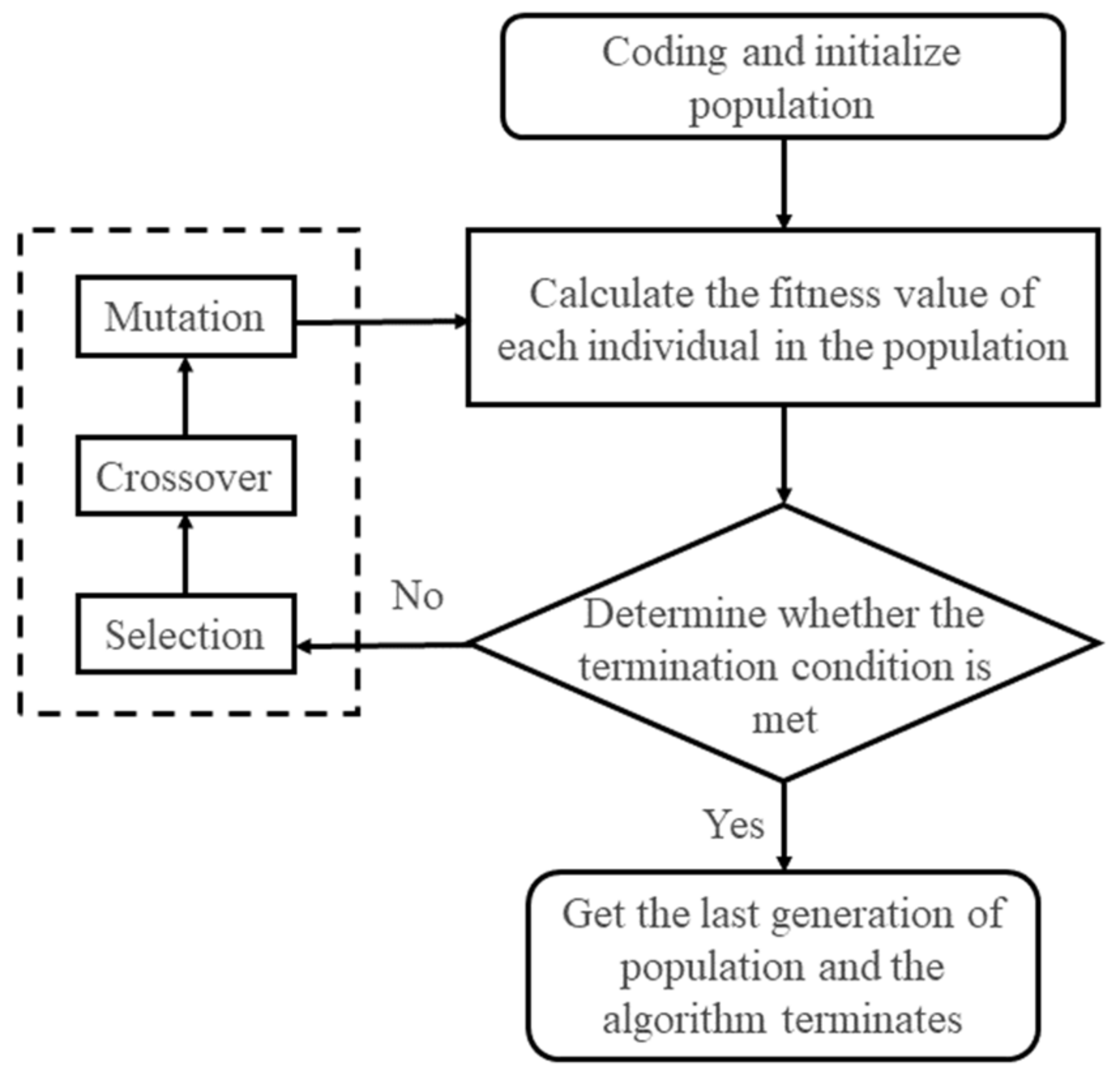
Here, the genetic algorithm is used to perform the optimal global search. A genetic algorithm (GA) is proposed by Holland [33] based on the natural selection and genetic mechanism of Darwinian biological evolution to obtain the optimal solution, which has been well applied in many fields. It first encodes the solution (called chromosome) of the problem, usually using binary encoding or real number encoding to map the solution space to the chromosome space as follows:

$$x_i={\mathrm{U}}_1+({\displaystyle \sum _{j=1}^m{b}_j}·2^{j-1})·\frac{{\mathrm{U}}_2{-\mathrm{U}}_1}{2^m-1}$$

(12)

where ${\mathrm{U}}_1$ and ${\mathrm{U}}_2$ denote the lower and upper limits of the value of parameter $x_i$, respectively, m is the length of the chromosome of encoded variable, and $b_j$ is the genetic coding at position j of the variable.

Subsequently, reasonable initial populations are generated in these solution spaces, and the initial populations are processed with crossover and mutation. Moreover, the kth individual fitness function is calculated as follows:

$$f_c(X_k)=\frac{1}{1+f_o(X_k)},k=1,2,\dots ,\mathrm{M}$$

(13)

where M is the number of populations.

In the following, the proportional selection operator $p_k$ is adopted to determine the likelihood of descendants being left behind. The probability that the kth individual will be selected in the next generation is calculated by fitness function as follows.

$$p_k=\frac{f_c(X_k)}{{\displaystyle \sum _{k=1}^M{f}_c(X_k)}},\hspace{1em}k=1,2,\dots ,\mathrm{M}$$

(14)

As improved individuals are selected based on selection operator $p_k$, the advantages of the previous generation are retained in the new generation. The calculation is repeated until the condition of convergence is met; thus, the optimization solution can be obtained. The basic principle of GA is shown in Figure 3.

The optimal combined strain response is used to identify the combined strain influence line according to Equation (15):

$$I_{\mathrm{z}}=A^{+}{\mathbf{\epsilon }}_{\mathrm{z}}={(A^{\mathrm{T}}A)}^{-1}{A}^{\mathrm{T}}{\mathbf{\epsilon }}_z$$

(15)

where ${\mathbf{\epsilon }}_z$ and $I_{\mathrm{z}}$ denotes combined strain responses and combined strain influence lines, respectively.

To reduce noise interference, multiple transverse positions loading can be performed to identify the corresponding combined strain influence lines, and the results are averaged.

2.4. Axle Weight Identification

For the unknown vehicle load, the above method is first used to identify the number of axles, N_A, the wheelbase, B_n, and the vehicle’s speed, v, and then according to the identified combined strain influence line, $I_{\mathrm{z}}$; the combined strain response can be expressed as follows.

$${\left[I\right]}_{({\mathrm{N}}_{\mathrm{I}}+C_{\mathrm{N}}{}_{{}_{\mathrm{A}}}-1)\times {\mathrm{N}}_A}{\left[A\right]}_{{\mathrm{N}}_{\mathrm{A}}\times 1}={\left[{\mathbf{\epsilon }}_z\right]}_{({\mathrm{N}}_{\mathrm{I}}+C_{\mathrm{N}}{}_{{}_{\mathrm{A}}}-1)\times 1}$$

(16)

$${\left[I\right]}_{({\mathrm{N}}_{\mathrm{I}}+C_{{\mathrm{N}}_{\mathrm{A}}}-1)\times {\mathrm{N}}_{\mathrm{A}}}=\left[\begin{array}{cccccc}{I}_{\mathrm{z}}& 0& \dots & 0& \dots & 0\\ 0& {\left[0\right]}_{(C_2-1)\times 1}& ⋮& ⋮& ⋮& ⋮\\ 0& 0& ⋮& {\left[0\right]}_{(C_n-1)\times 1}& ⋮& ⋮\\ ⋮& {\mathbf{I}}_z& ⋮& ⋮& ⋮& {\left[0\right]}_{(C_{{\mathrm{N}}_{\mathrm{A}}}-1)\times 1}\\ ⋮& 0& \dots & 0& \dots & ⋮\\ {\left[0\right]}_{(C_{{\mathrm{N}}_{\mathrm{A}}}-C_1)\times 1}& ⋮& ⋮& {\mathbf{I}}_z& ⋮& ⋮\\ ⋮& {\left[0\right]}_{(C_2-C_1)\times 1}& \dots & 0& \dots & 0\\ ⋮& ⋮& ⋮& {\left[0\right]}_{(C_n-C_1)\times 1}& ⋮& 0\\ 0& 0& \dots & 0& \dots & {\mathbf{I}}_z\end{array}\right]$$

(17)

$${\left[A\right]}_{{\mathrm{N}}_{\mathrm{A}}\times 1}={\left[A_1\hspace{0.33em}\hspace{0.33em}{A}_2\hspace{0.33em}\dots \hspace{0.33em}\hspace{0.33em}{A}_{{\mathrm{N}}_{\mathrm{A}}}\right]}^{\mathrm{T}}$$

(18)

Thus, the unknown vehicle axle weight can be estimated from the combined strain response using the least squares method.

$$A=I^{+}{\mathbf{\epsilon }}_z={(I^{\mathrm{T}}I)}^{-1}{I}^{\mathrm{T}}{\mathbf{\epsilon }}_z$$

(19)

The sum of the axle weights gives the gross vehicle weight.

3. Numerical Simulation

To verify the effectiveness of the proposed method, a local finite element model is established here for an actual orthotropic deck steel box beam bridge, and a numerical simulation is used to analyze the structural response when a vehicle passes the bridge. The response is used for unknown vehicle load identifications.

3.1. Model Building

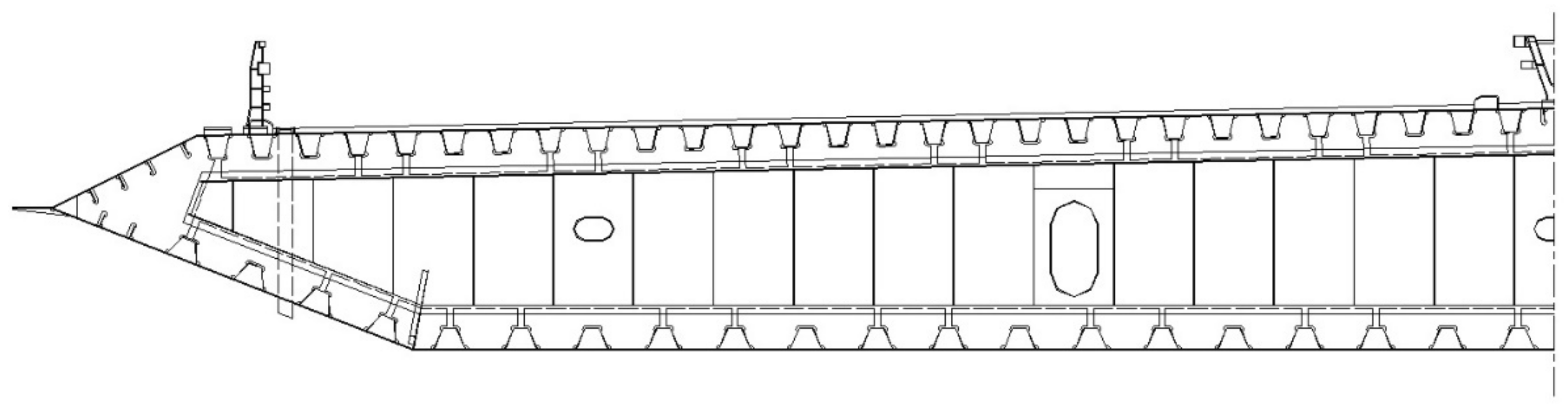
The half-span cross-section of an actual orthotropic deck steel box girder is shown in Figure 4. Considering the local force feature of the orthotropic deck, a partial structure is intercepted here to establish a local finite element model. The model has two lanes with a width of 7.5 m in the horizontal direction, five-span diaphragms with a length of 16 m in the longitudinal direction, and part of the diaphragm with 2 m down from the deck in the vertical direction. The deck, U-rib, and diaphragm thicknesses are 14 mm, 12 mm, and 8 mm, respectively. All components of the model are simulated using shell elements. 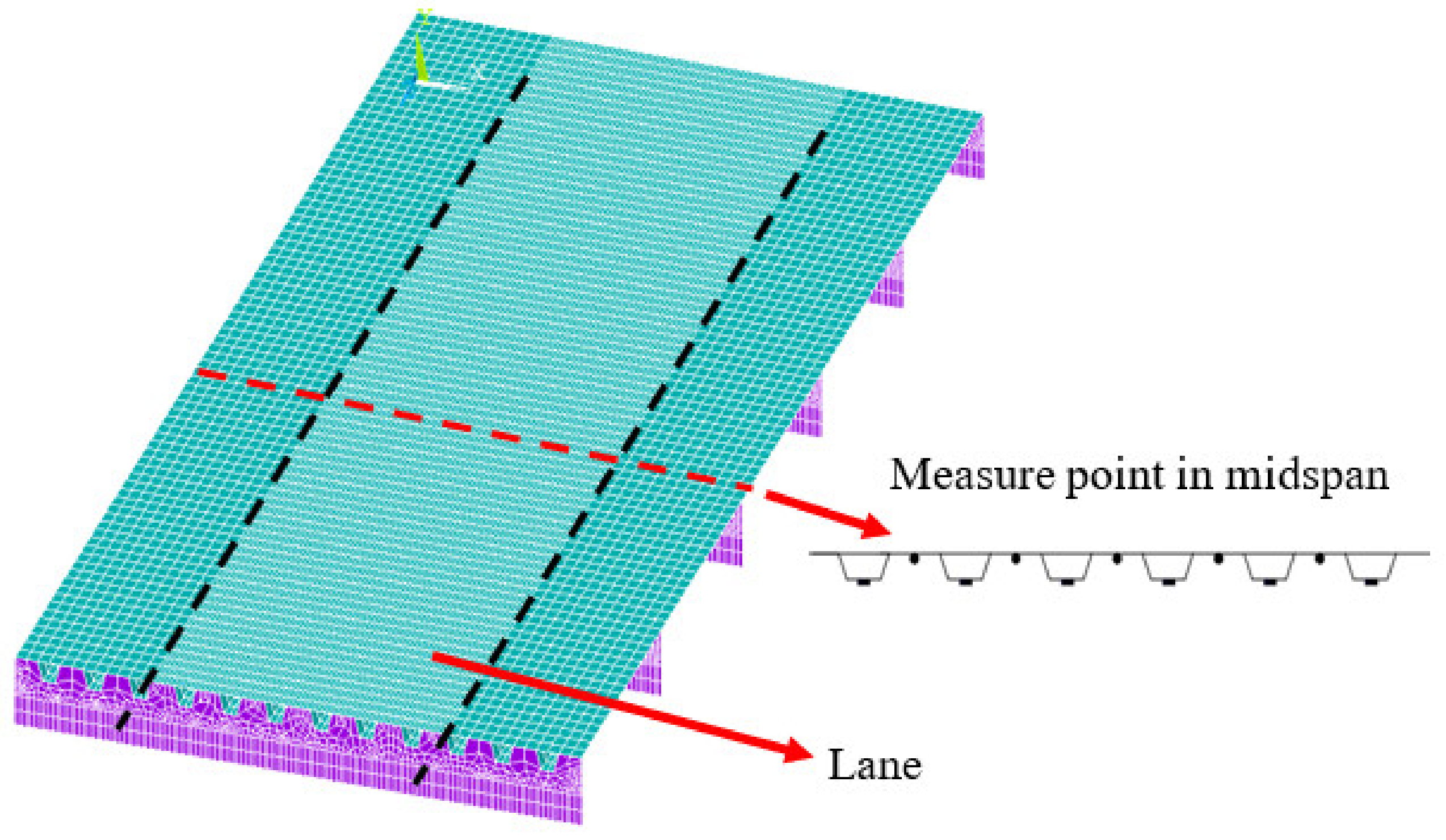The elasticity modulus of the material is $\mathrm{E}=2.1\times {10}^{11}$ Pa-. Here, the research focuses on the load identification of a vehicle driving in one lane, so the mesh size of the middle lane is refined with an element size of 5 cm, and the other part of the deck is meshed with an element size of 15 cm. The bottom of the diaphragm is simply supported at the outermost end. The entire finite element model is shown in Figure 5. The response at the position of measurement points shown in Figure 1 is calculated by finite element analyses.

For the built FEM model of the orthotropic deck steel box girder, the deck comprises a panel and U-rib, and it has different stiffnesse in longitudinal and transverse directions. The deck is supported on multiple diaphragms, and its mechanical performance in longitudinal direction is similar to continuous rigid frame bridges under local wheel loads. The strain influence line of U-rib is short, and it will vary with the transverse position of the vehicle. Because the transverse stiffness of the deck is smaller than longitudinal stiffness, the strain influence line of the panel is more localized, which is suitable for axle identification.

3.2. Axle Information Identification

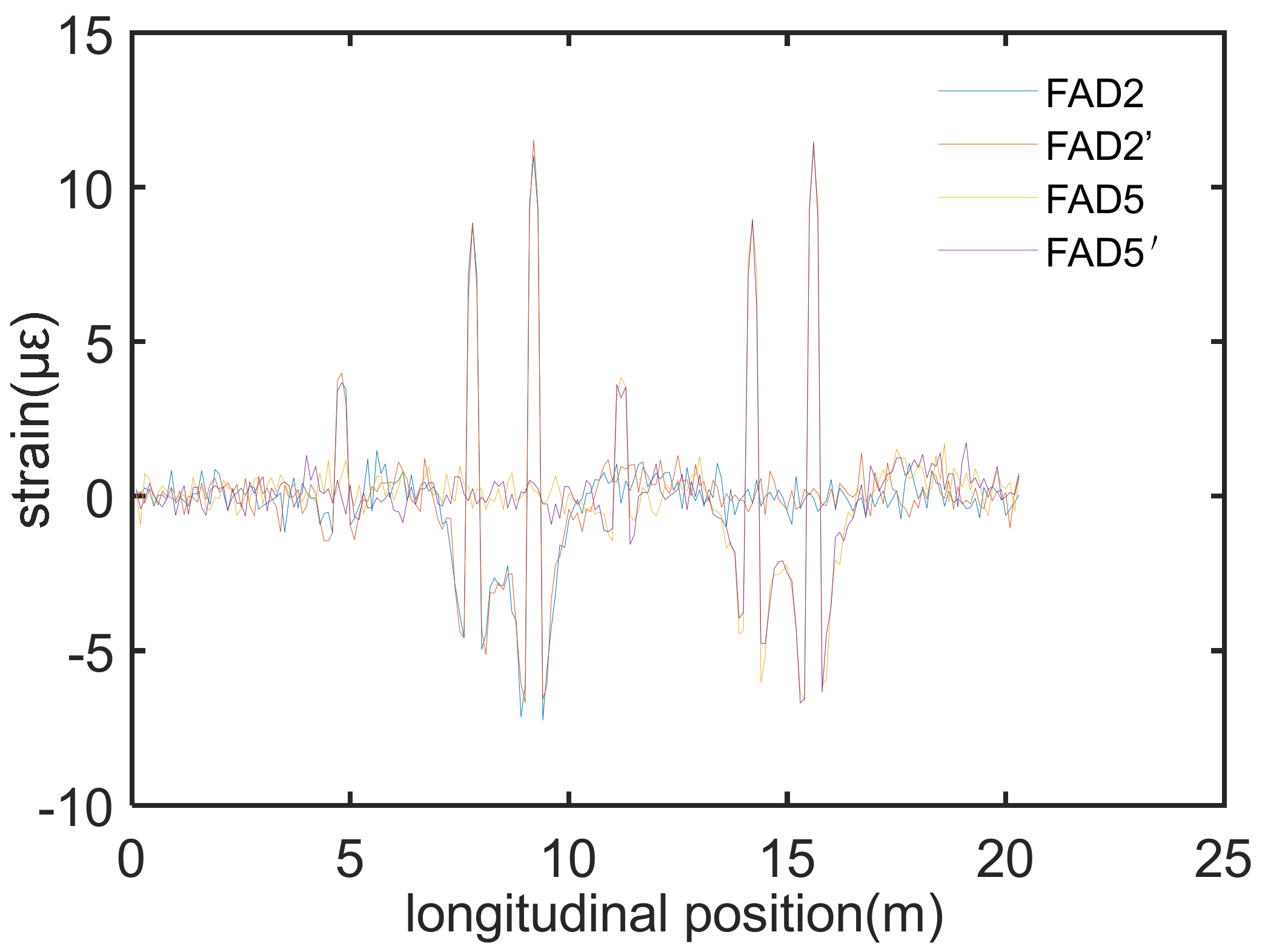
The vehicle’s load is applied on the deck along the longitudinal direction to simulate a vehicle passing on bridge. Here, a three-axle vehicle with a gross weight of 35 kN is taken to pass the bridge, and the strain response at the position of FAD sensors shown in Figure 1 is calculated by finite element analyses (FEA). The weight of the front, middle, and rear axles is 5 kN, 13 kN, and 17 kN, respectively. The wheel track of the vehicle is180 cm. The front and rear wheelbase is 300 cm and 140 cm, respectively. To consider the noise effect, a noise of 20% (defined as noise variance/signal variance) is added to the strain response, and the response of part of the sensors is shown in Figure 6.

As observed the figure, three pronounced peaks occur when the axle passes through the FAD sensor, which correspond to three axles. The identified wheelbases by the proposed algorithm are 3.0 m and 1.2 m, respectively, which validated the effectiveness of the proposed method.

3.3. Calibration of Influence Line

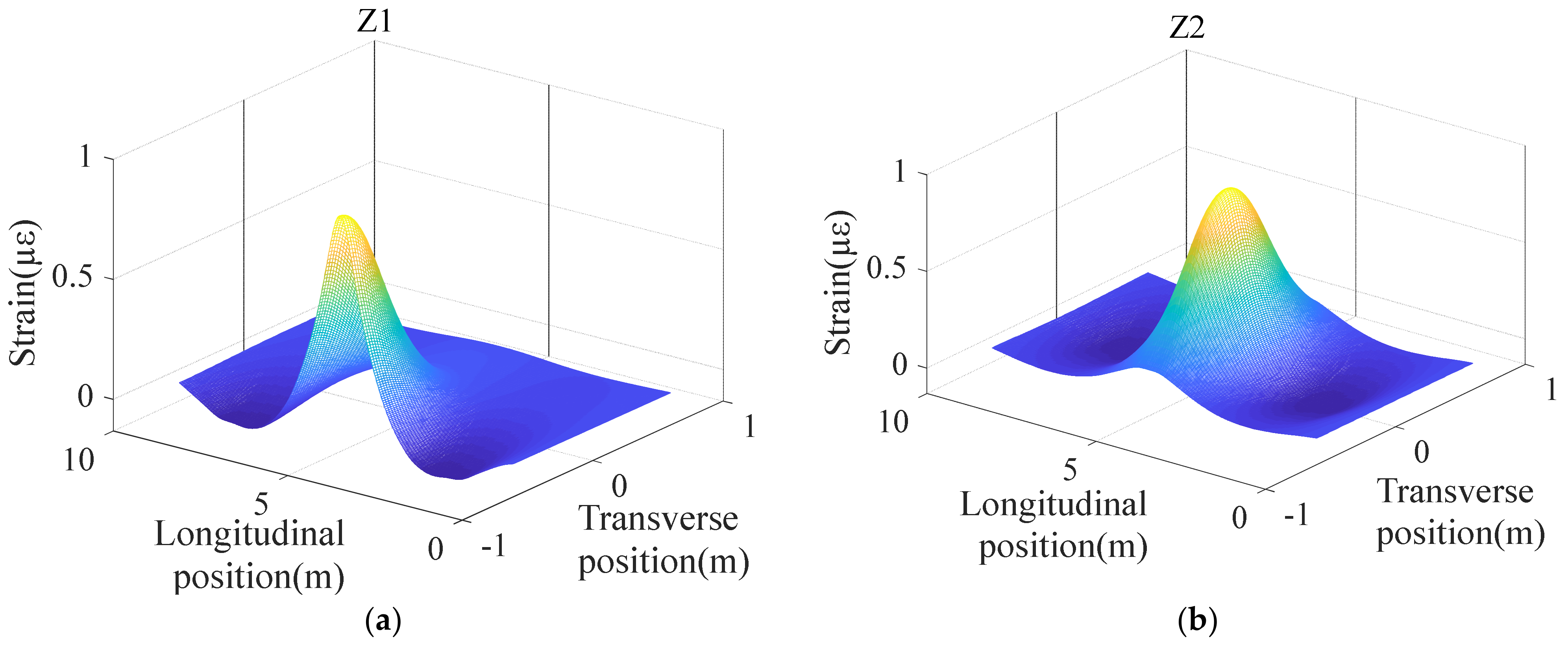
Taking the center position of the bridge deck as x = 0, a two-axle vehicle with a gross weight of 25 kN, a front and rear axle weight of 10 kN and 15 kN, respectively, and a wheelbase of 320 cm is driven across the bridge every 5 cm from x = −0.8 m to x = 0.8 m along the transverse position. The strain response at the position of the axle weight sensors shown in Figure 5 is calculated by FEA. Thus, the strain influence lines of each sensor under vehicle load at different transverse positions can be identified. The identified influence lines of Z1 and Z2 is shown in Figure 7 below.

As seen from the above figure, the influence line will be affected by the transverse position of the vehicle’s load. For precisely identifying the vehicle’s load, it is necessary to accurately identify the transverse position of the vehicle’s load, which is not convenient for practical engineering applications. Therefore, the proposed GA optimization method is adopted to find an optimal combination of measurement point responses that are insensitive to the vehicle load’s transverse position. The relevant parameter of GA is listed in

Table 1. The relevant parameter of GA.

Parameter	Value
Maximum number of genetic generations	1000
Population size	50
Encoding method	Binary encoding
Selection method	Roulette
Crossover approach	Uniform crossover
Mutation method	Multipoint mutation
Crossover probability	0.8
Mutation probability	0.2
Range of independent variables	(−20, 20)
Deviation of fitness function value	1 × 10−6

.

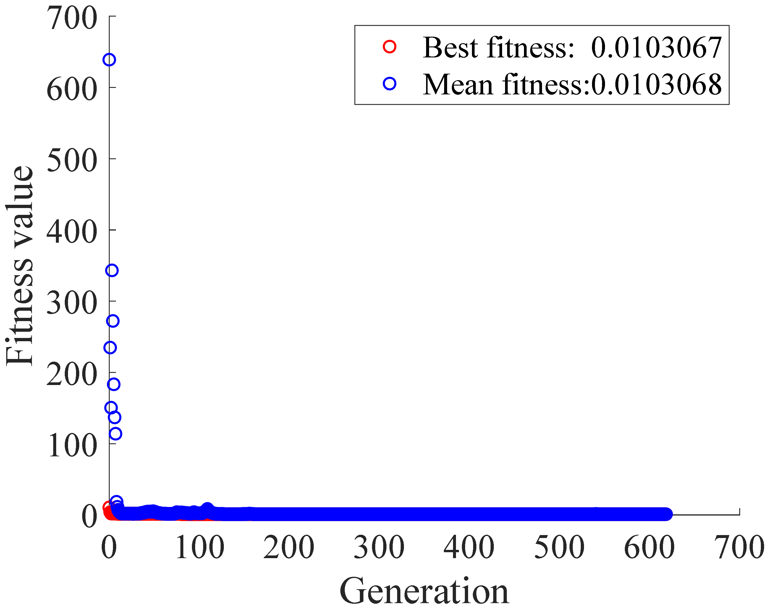
The result of the optimization iteration is shown in Figure 8.

After GA global optimization, we can obtain the optimal combination coefficients of six measurement points as $k_i$ = [−2.599, 4.758, 4.233, 4.965, −2.302, −1.865].

The optimal combined strain response is used to identify the corresponding combined strain influence line under the vehicle load at different transverse positions. The identified result is shown in Figure 9.

As observed from the figure, the optimal combined strain influence line does not change much when the vehicle passes the bridge at different transverse positions, so it is not sensitive to the lateral position of the load. It can be used for vehicle load identification without identifying the transverse position of the load. The optimal combined strain influence line identified under load at different transverse positions is averaged, which will be used for the following identification of axle weights.

3.4. Axle Weight Identification

To verify the identification effect of the proposed method on the axle’s weight, different vehicle loads were driven across the bridge from different transverse positions. The strain response of each measurement point was obtained by using finite element simulation analysis. A total of three types of vehicles were simulated, each with five cases and the vehicle parameters under various cases were listed in

Table 2. The parameter of the two-axle vehicle under different cases.

Case	TP (cm)	Wheelbase (m)	Axle Weight (kN)
		D1	A1	A2
1	−68	2.4	7	14
2	−42	2.6	14	14
3	8	2.8	14	21
4	34	3	14	28
5	50	3.2	21	28

Note: TP denotes the transverse position of the vehicle load, D1 denotes the first wheelbase, and A1 denotes the weight of the first axle, which is the same as the others.

,

Table 3. The parameter of the three-axle vehicle under different cases.

Case	TP (cm)	Wheelbase (m)		Axle Weight (kN)
		D1	D2	A1	A2	A3
1	−68	2.6	1.2	7	14	14
2	−42	2.8	1.4	14	14	14
3	8	3	1.4	14	14	21
4	34	3.2	1.2	14	14	28
5	50	3.2	1.4	14	28	28

and

Table 4. The parameter of the five-axle vehicle under different cases.

Case	TP (cm)	Wheelbase (m)				Axle Weight (kN)
		D1	D2	D3	D4	A1	A2	A3	A4	A5
1	−68	3	1.2	6	1.2	7	14	14	14	21
2	−42	3	1.4	6	1.4	14	14	14	14	21
3	8	3.2	1.4	6	1.4	14	14	21	21	21
4	34	3.2	1.4	5	1.4	14	14	21	28	28
5	50	3.4	1.4	6	1.4	14	28	28	28	28

, respectively.

The proposed method was used to identify the unknown axle loads based on the identified combined strain influence lines, and the identified results are listed in

Table 5. The identified result of the two-axle vehicle.

Case	Identified Error (%)
	A1	A2	GVW
1	0.30	1.01	0.77
2	−0.64	−0.33	−0.48
3	−0.75	−0.20	−0.42
4	1.11	1.14	1.13
5	1.36	1.46	1.42
Mean	0.83	0.83	0.84

Note: The GVW denotes the vehicle’s gross weight. The following are the same. The mean is the average of the absolute error, which is the same as follows.

,

Table 6. The identified result of the three-axle vehicle.

Case	Identified Error (%)
	A1	A2	A3	GVW
1	0.68	1.20	0.95	1.00
2	0.66	0.17	0.37	0.40
3	1.84	0.82	0.42	0.94
4	2.31	2.03	0.87	1.52
5	−0.22	0.21	2.46	1.02
Mean	1.14	0.87	1.01	0.98

and

Table 7. The identified result of the five-axle vehicle.

Case	Identified Error (%)
	A1	A2	A3	A4	A5	GVW
1	0.70	−0.26	2.08	2.32	0.54	1.06
2	0.26	0.02	−0.85	1.53	−0.78	−0.04
3	1.22	−2.50	−0.41	−0.22	−2.90	−1.01
4	0.89	−0.81	1.64	1.74	0.19	0.85
5	0.36	1.10	1.96	2.51	1.31	1.57
Mean	0.69	0.94	1.39	1.66	1.14	0.91

.

It can be seen from the results that the maximal identified error of the axle’s weight is below 2% and that of the gross weight is below 1%. The main cause is that the identified errors of some axles are positive while other axles are negative. This indicated that the optimized combined influence line is insensitive to the transverse position of the vehicle. The proposed algorithm can be used to identify vehicle loads without estimating the transverse position of the vehicle in advance.

4. Experimental Verification

4.1. Test Model

In order to further verify the effectiveness and accuracy of the proposed method, a 1:6 scale-down model test was designed according to the numerical simulated orthotropic steel box girder model, which consisted of a deck, U-rib, and diaphragm. The model is 270 cm long, 83 cm wide, and 20 cm high, with six U-ribs under the deck and six diaphragms with a spacing of 54 cm. The diaphragms are truncated vertically, so the model has no bottom plate, and all diaphragms are connected by two steel bars. The model is made of Q235 hot-rolled steel plate, and the thickness of all steel plates is 2 mm. The steel beam model is simply supported by a cushion at the bottom of the first and last diaphragm. To ensure that the test vehicle can pass the steel box beam model at a uniform speed, lead and tail beam were installed at the beginning and end of the steel box beam. The lead and tail beams are located as close as possible to the steel box girder but disconnected from the steel box girder.

It should be noted that the designed experimental model does not strictly meet the similarity ratio criterion. However, the study does not focus on the absolute force condition of the structure. For different scale models, the measured strain response maybe different with practical engineering structures. However, the local force characteristic of the orthotropic deck is similar, and the strain influence line is short. We can identify the strain influence line and the optimized parameters corresponding to different scale models using the proposed method, and then we can verify the proposed method based on the identified results.

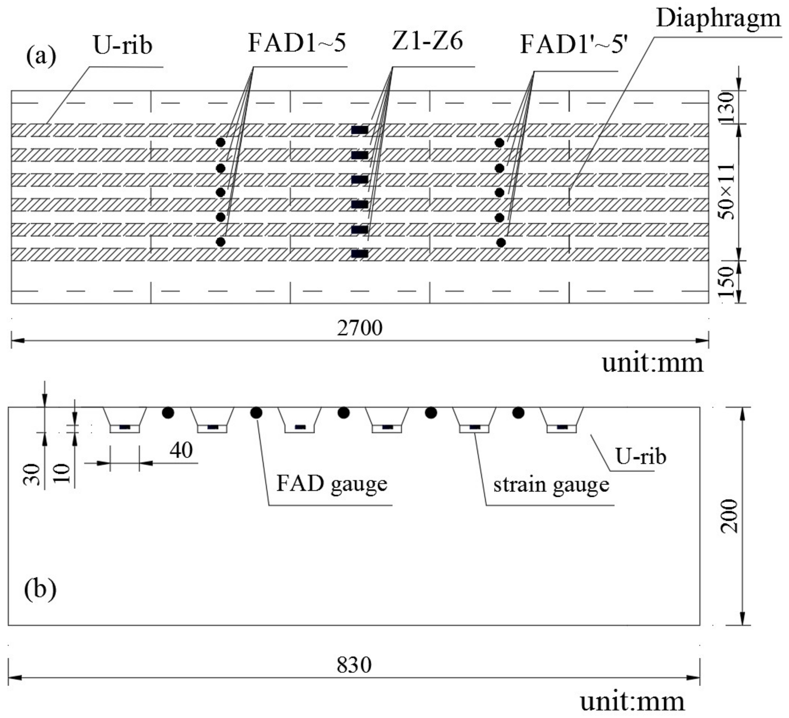
Six axle weight sensors are placed on the lower edge of the span of each of the U-ribs in the middle section of the model, and ten FDA sensors are placed on the lower edge of the deck between adjacent U-ribs. Detailed dimensions and layouts of measurement points are shown in Figure 10.

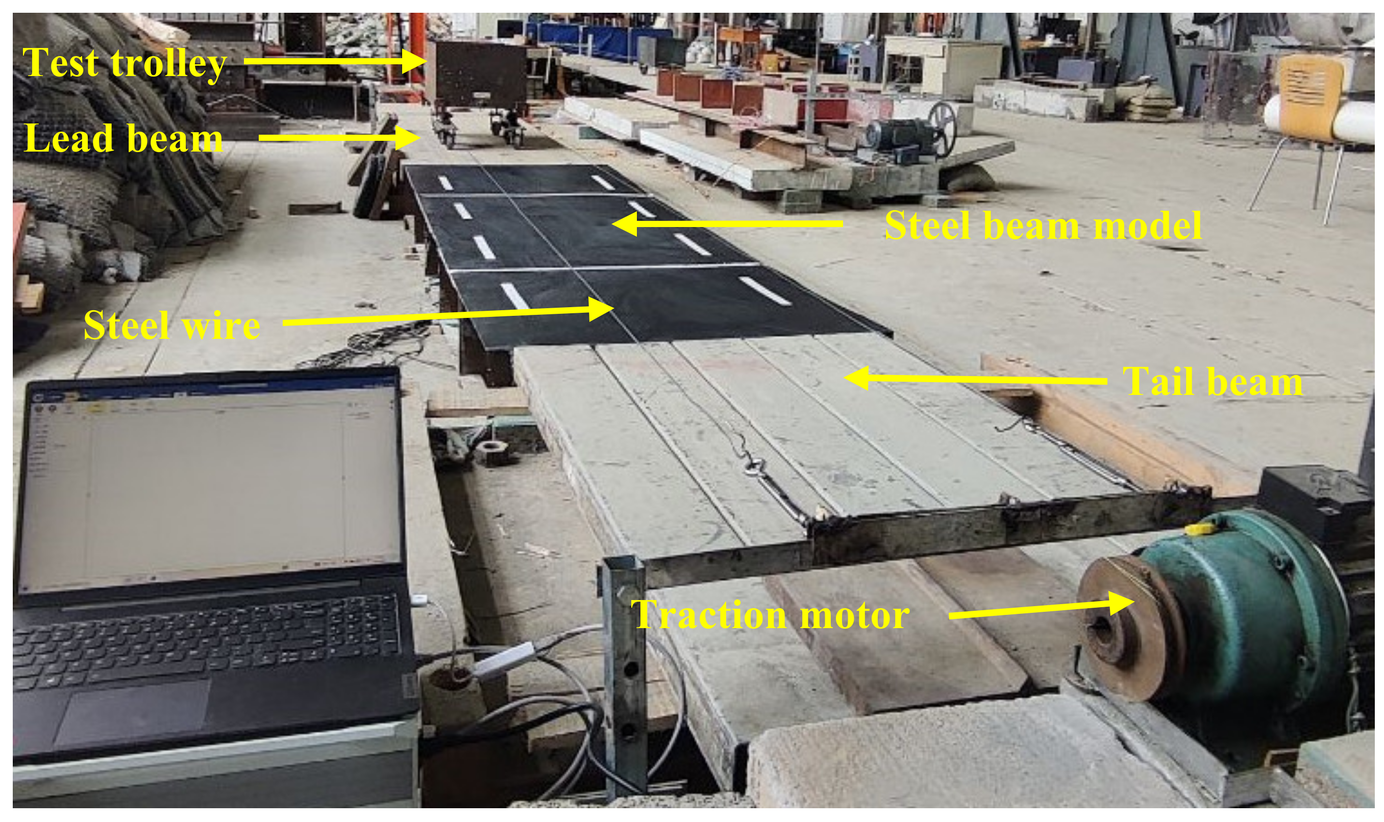
A two- and three-axle vehicle was designed to simulate a vehicle’s load. The vehicle’s tread was 28 cm, the wheel width was 2 cm, the wheelbase can be adjusted, and the axle weight and gross weight can be changed by adding mass blocks to the vehicle. In order to ensure that the experimental trolley drives through the steel beam model in a straight line as much as possible, two limit holes are set on the experimental trolley, and two steel wires that can move laterally are fixed above the steel beam model. The wires pass through the limit holes of the trolley. A motor was fixed at the end of the tail beam, and the motor dragged the trolley through the experimental steel box beam at a uniform speed. The entire experimental model is shown in Figure 11.

4.2. Identification of Axle Information

A known calibration vehicle is first driven through the steel beam model from different transverse positions by a motor traction to identify the axle’s weight. The calibration vehicle was a two-axle vehicle with a gross weight of 50.8 kg and front and rear axles of 26.2 kg and 24.6 kg, respectively. The center position of the vehicle acting on the beam model is defined as x = 0 cm, and a total of 47 transverse positions (x = −13.5~12.0 cm) were tested; FAD sensors and axle weight sensors collected corresponding strain responses. 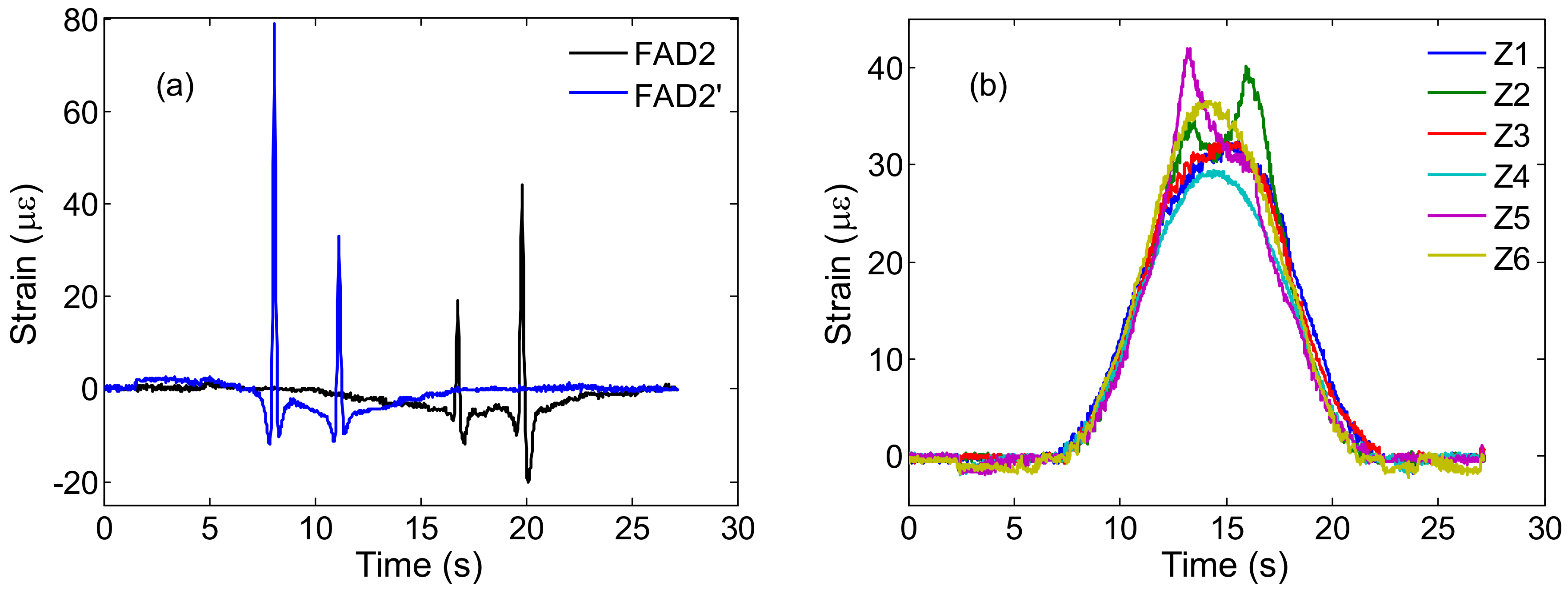Figure 12 shows part of the strain response when the calibration vehicle passes on the steel beam model from a transverse position of x = −1.5 cm.

It can be seen that FAD sensors monitor two distinct peak points, which correspond to the two axles of the calibrated vehicle. Based on the proposed method, the wheelbase and the vehicle’s speed can be estimated.

Table 8. Part of identification results of axle information.

Testing	Speed (cm/s)	Practical Wheelbase (cm)	Identifying Wheelbase (cm)	Error (%)
1	12.26	38	37.68	−0.84
2	12.34		38.25	0.66
3	12.34		38.13	0.34
4	12.44		37.82	−0.47
5	12.37		37.98	−0.05
6	12.44		37.82	−0.47
7	12.40		38.07	0.18
8	12.47		37.91	−0.24
Mean	12.38		37.96	0.41

Note: The mean is the average of the absolute error.

shows part of the identification results.

As observed from the above table, the identified speed varies in a range of 12.26~12.47 cm/s, and the mean speed is 12.38 cm/s. The identified wheelbase range is 37.68~38.25 cm, and the mean of identified error is 0.41%, which indicates that the identified speed and wheelbase have good stability and accuracy.

4.3. Calibration of Combined Strain Influence Line

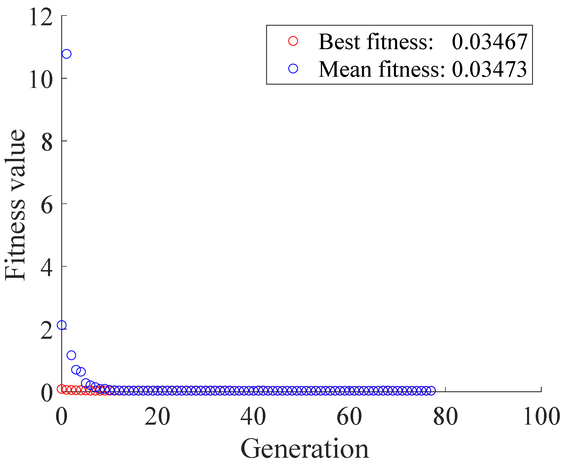
For the 47 sets of strain responses collected from the calibration vehicle test, the GA-proposed optimization method was used to determine the optimal combination of strain responses. The result of the optimization iteration is shown in Figure 13.

The minimum variation coefficient after GA global optimization is 0.03467, and the optimal combinations coefficients of six measurement points are $k_i$ = [9.645, 4.017, 1.255, 2.071, 14.709, 8.456].

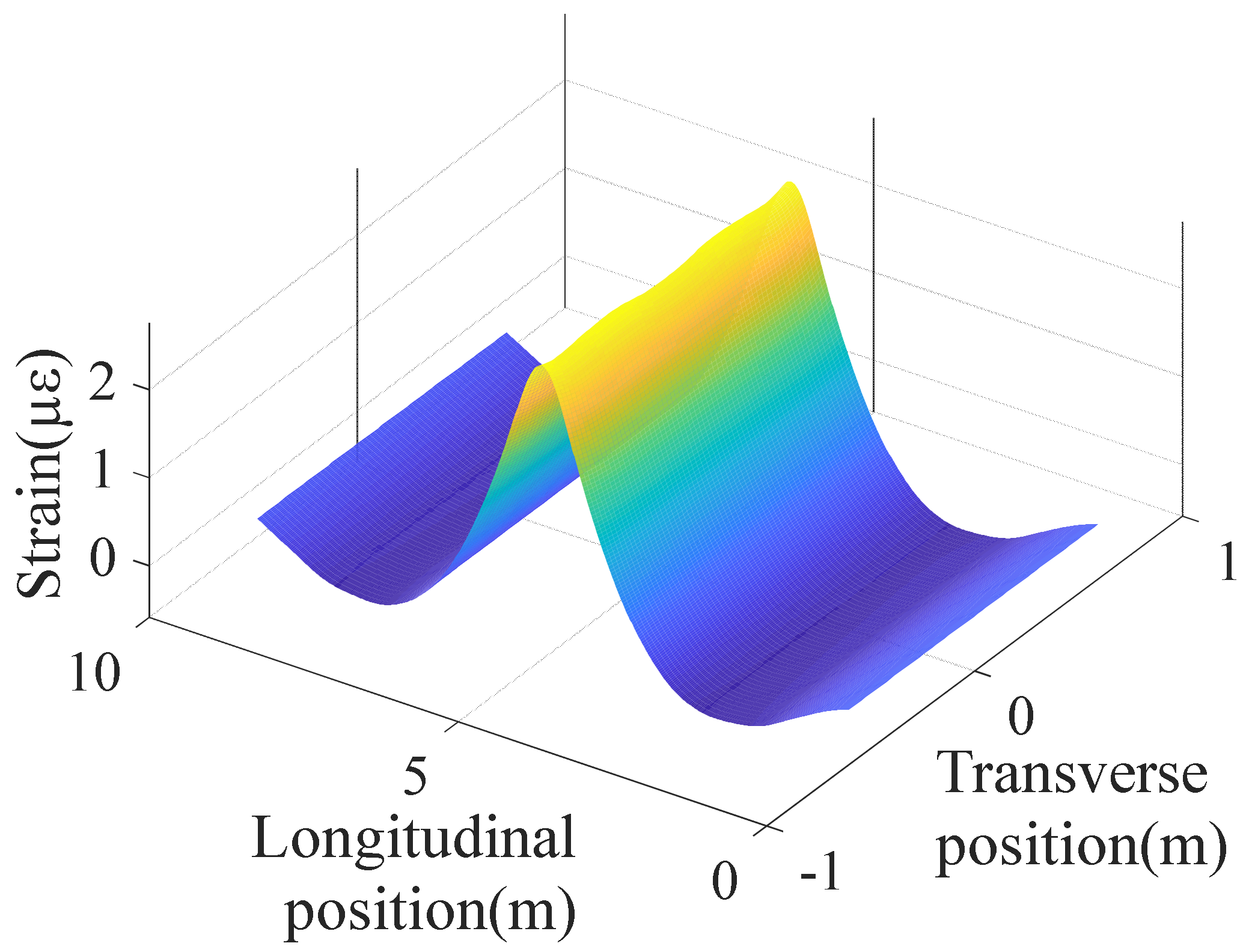
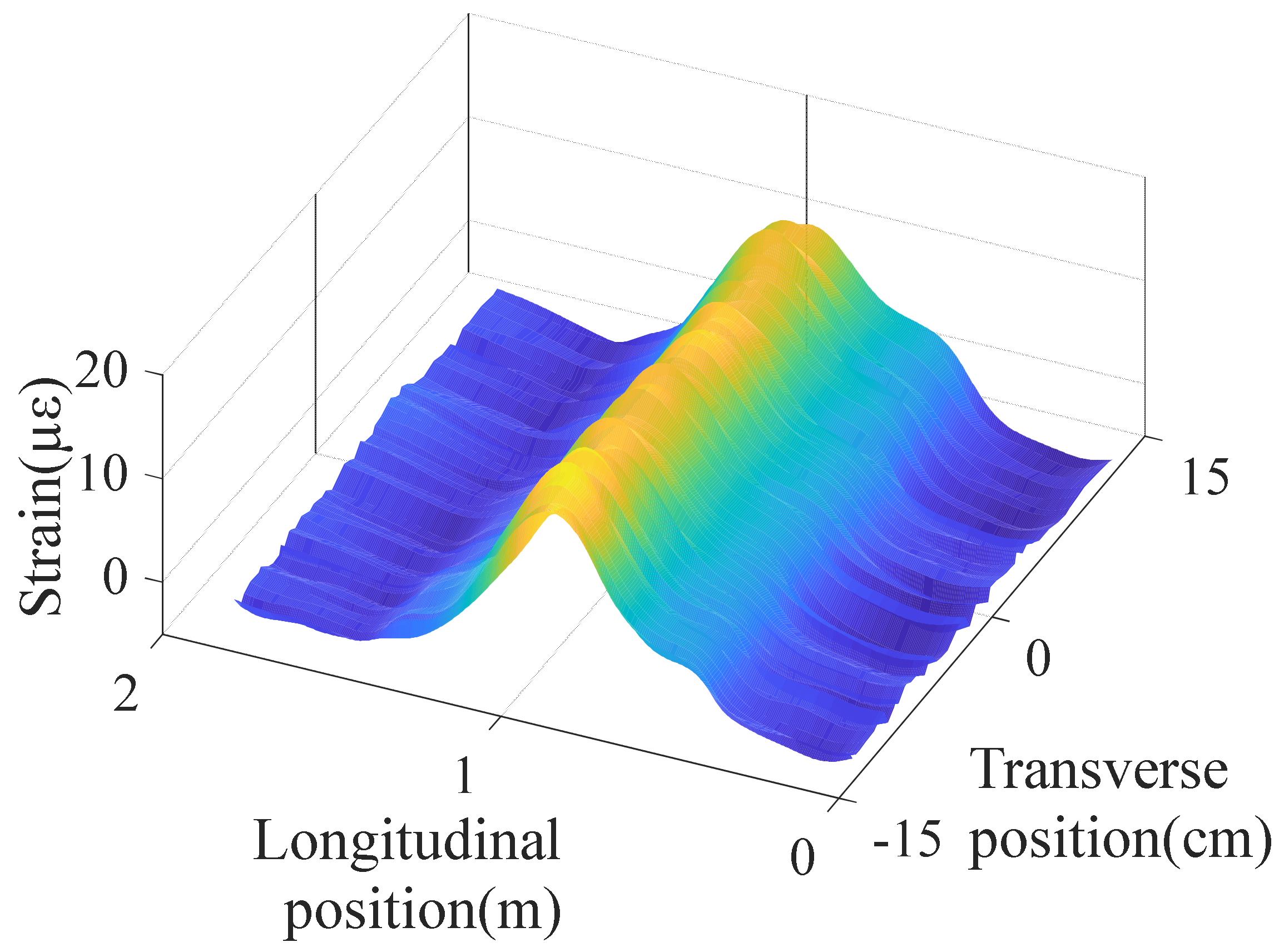
The optimal combined strain response is used to identify the optimal combined strain influence line under the vehicle load at different transverse positions. The combined strain influence line takes the length of the middle three diaphragms from the second diaphragm on the left to the fifth diaphragm in Figure 9, and the position of the second diaphragm is defined as zero along the longitudinal bridge direction. The identified results are shown in Figure 14.

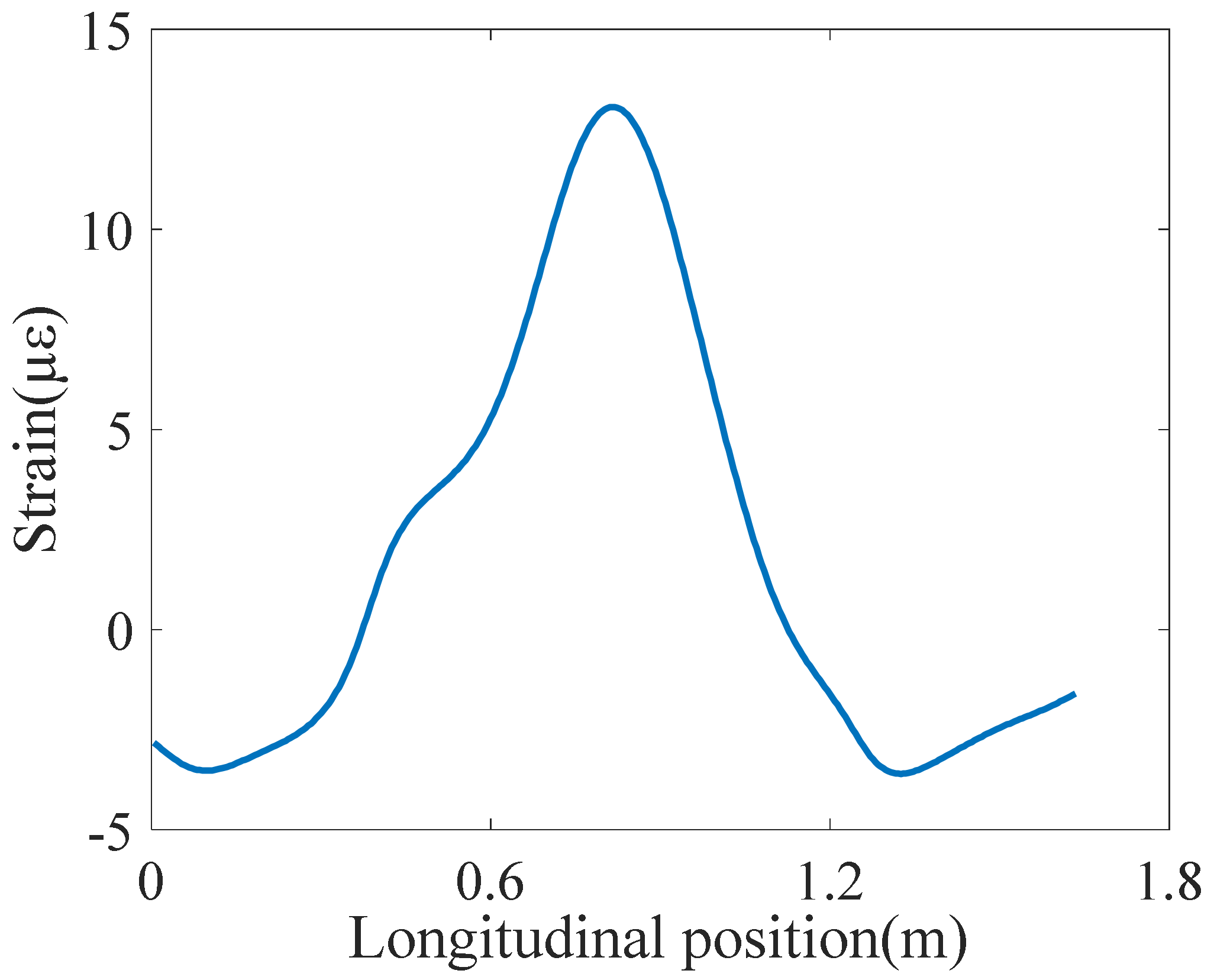
It can be seen that the combined strain influence line has good stability when the calibration vehicle is in different positions in the transverse direction. To simplify the axle weight load identification, the influence of the transverse position of the vehicle load can be disregarded. In order to reduce noise interferences, the combined influence lines at multiple transverse positions are averaged for the subsequent axle weight load identification, and the averaged result is shown in Figure 15.

As shown in the figure, the strain influence line is incomplete, symmetric, and smooth. The main reason is that the steel plate of the model is too thin (2 mm), so the welding leads to some deformations and local unevenness in the model. In addition, the vibration noise of the vehicle traveling on the uneven deck also introduces some identified errors.

4.4. Identification of the Axle Weight

Multiple tests were carried out using different configurations of two-axle and three-axle vehicles at different transverse positions. The detailed parameters of the vehicle are listed in

Table 9. Parameters of two- and three-axle vehicles.

Vehicle	Wheelbase (cm)		Axle Weight (kg)			GVW (kg)
	L1	L2	A1	A2	A3
Veh1	38.0	-	26.2	24.6	-	50.8
Veh2	38.0	-	45.3	32.7	-	78.0
Veh3	21.0	45.0	12.4	12..4	35.1	59.9
Veh4	21.0	53.0	16.35	16.35	28.8	61.5

Note: L1 denotes the first wheelbase, and A1 denotes the weight of first axle, which is same as the others.

.

Based on the optimal combined strain influence line, the axle and gross weight of the different test vehicles were identified, and the results are listed in

Table 10. The identified results of test vehicles.

Test ID	Vehicle	Transverse Position (cm)	Identification Error (%)
			A1 (kg)	A2 (kg)	A3 (kg)	GVW (kg)
1	Veh1	−12.6	5.77	3.41	-	4.63
2	Veh1	−4.2	−2.79	−7.16	-	−4.90
3	Veh2	5.2	−5.24	4.73	-	−1.06
4	Veh2	−5.2	−1.12	−5.35	-	−2.89
5	Veh3	10.4	2.79	1.99	−3.63	−1.13
6	Veh3	11.2	3.67	−6.17	3.43	1.50
7	Veh4	−10.2	3.16	−5.10	−3.44	−2.12
8	Veh4	3.8	−6.92	3.73	3.51	0.79

.

As listed in the table, the maximal identified error of the axle weight is about 5.8%, and that of the gross weight is about 4.9%. Due to the influence of the local unevenness of the model and measuring noise, the experimental test’s identified error is slightly larger than that of the numerical simulation. However, the current identification accuracy can meet practical engineering applications.

5. Conclusions

This paper proposed a vehicle load identification method based on an optimal combined strain influence line. Two types of strain sensors were installed on the deck and U-ribs to monitor the structural response for detecting the axle information and axle weight, respectively. To decrease the influence of the transverse position of the load, an optimal combined strain influence line was proposed using a genetic optimization algorithm based on an index of variation coefficient. Then, the vehicle load could be identified based on a calibrated combined strain influence line using the least squares method. From numerical and experimental results, some conclusions can be drawn as follows:

(1)

The axle’s information can be accurately identified based on the FAD sensors installed on the lower edge of the deck between the U-ribs.

(2)

The index of variation coefficient can be used to evaluate the sensitivity of the transverse position of the vehicle to the strain influence line. Based on the index, the optimized combined influence line searched by the genetic algorithm is, to some extent, insensitive to the transverse position of the vehicle.

(3)

Axle weight and gross weight identification errors for numerical simulation are below 2% and 1%, respectively, and that of the experimental test are below 5.8% and 4.9%, respectively. The maximal identified error of axle weight is larger than that of the gross weight, and the main cause is that the identified errors of some axles are positive while other axles are negative. The experimental test’s identified error is slightly larger than that of the numerical analysis due to the welding deformation and measuring noise. However, the identification accuracy insufficient for meeting the demand of practical engineering applications.

(4)

Overall, the proposed optimized combined influence line algorithm can effectively and accurately identify the vehicle’s load on the orthotropic deck steel box beam bridge without estimating the transverse position of the vehicle in advance, which is convenient for engineering applications.