Clustering Analysis for Classifying Student Academic Performance in Higher Education

Abstract

There are three income categories for Malaysians: the top 20% (T20), the middle 40% (M40), and the bottom 40% (B40). The government has extended B40′s access to higher education to eliminate socioeconomic disparities and improve their lives. The number of students enrolled in bachelor’s degree programmes at universities has risen annually. However, not all students who enrolled graduated. Machine learning approaches have been widely used and improved in education. However, research studies related to unsupervised learning in education are generally lacking. Therefore, this study proposes a clustering-based approach for classifying B40 students based on their performance in higher education institutions (HEIs). This study developed three unsupervised models (k-means, BIRCH, and DBSCAN) based on the data of B40 students. Several data pre-processing tasks and feature selection have been conducted on the raw dataset to ensure the quality of the training data. Each model is optimized using different tuning parameters. The observational results have shown that the optimized k-means on Model B (KMoB) achieved the highest performance among all the models. KMoB produced five clusters of B40 students based on their performance. With KMoB, this study may assist the government in reducing HEI drop-out rates, increasing graduation rates, and eventually boosting students’ socioeconomic status.

1. Introduction

The explosive growth of educational data in recent years has fostered data-driven actions concerning education quality improvement in public Higher Education Institutions (HEIs) by discovering patterns and knowledge. The increase in the quantity of data also challenges researchers to ensure that the performance of the machine learning algorithm developed is the best and can solve problems accurately. Every year, the total quantity of student data in the education sector increases dramatically. These are gigantic data and contain crucial information, making it impossible to analyse manually. So, tools and approaches that can automatically analyse these data are needed to derive hidden patterns and knowledge that could be of great use to provide insights into student performance. In turn, educators can leverage this information to help improve students’ performance.

Most recently, educational data mining has been regarded as a very useful tool in analysing and predicting the behaviour and performance of students in the future [1]. In addition, the use of learning analytics has also grown due to the significant increase in data quantity, improved data formats, computer advancements, and the availability of advanced analysis tools [2]. Predicting the performance of students as well as the drop-out rate in education is very important at the higher education level, especially in public universities. Due to uncertain economic conditions, higher education institutions (HEIs) had to cut expenses but enhance their quality and efficiency even before the COVID-19 pandemic. Thus, the key aim for ensuring the sustainability of higher learning institutions is to retain the number of students during student enrolment until the end of the course.

B40 represents the lowest household group, with an average income below RM4850 per month [3]. One of the Eleventh Malaysia Plan (11 MP) objectives is to advance the B40 household group to the middle-income group. According to the available statistics, the number of students enrolled in bachelor’s degree programmes at Malaysia’s universities has been increasing annually. Despite a large number of enrolments, not all students can graduate on time. Students dropping out of the university will negatively affect B40 families financially. The family financial burden will increase as students’ education loan has to be paid even if they fail to graduate.

Furthermore, it will affect a student’s chances of securing a high-income job. Student drop-out would also lead to a huge loss in human capital in the nation as fewer professionals and public universities will produce expert skills. Thus, to improve the standard of living among this group, the achievements and performance of B40 students in public HEIs need to be given more attention.

Lately, machine learning techniques have been widely applied in forecasting student performance at various levels of study. Most studies use supervised classification approaches to generate predictions. Previous studies focused on developing unsupervised machine learning models by predicting student performance using student data sets from online learning systems. Clustering techniques have been used to predict student performance; however, the data set only includes student performance from online learning, which does not represent B40 students, as B40 students do not have the ease of access to online learning. Research related to unsupervised machine learning to cluster B40 students based on their performance, behaviour, and achievement in HEI is generally lacking. Student behaviour factors were poorly considered in predicting drop-out among B40 households in public universities. This new dimension of student behaviour will look at the number of curriculum activities students participate in during their university studies. Therefore, this study proposes a clustering-based approach for classifying B40 based on their performance, behaviour (i.e., the number of student curriculum activities), and achievement in public HEIs. This study developed three unsupervised machine learning models (k-means, BIRCH, and DBSCAN) based on demographic, co-curricular activities, awards, industrial training, and employment data of B40 students. The following contributions made by this paper have been summarized as follows:

• Employing the most effective developed clustering algorithm, it has identified five clusters based on B40 student performance in Higher Education Institutions.
• B40 Student dataset used in this research was provided solely for this study and had never been used previously.
• It demonstrated that the B40 student dataset contains significant features that lead to academic performance.

The dataset used in this study was obtained from the Policy Planning and Research Division, Ministry of Higher Education (MOHE), consisting of student demographic, behavioural factors, participation in co-curricular activities, academic achievement, awards, industrial training, and employment data of B40 students. The dataset is used to train and validate each model. A clustering evaluation metric measures the better-defined cluster and spacing between clusters. The classification models (i.e., artificial neural network, random forests, and decision tree) will then be developed to classify the B40 students based on their performance as clustered by the KMoB model.

The remainder of this paper is organized as follows. Section 2 presents previous research articles on clustering and student performance in higher learning institutions. Section 3 describes the data pre-processing and development of clustering models using k-means, BIRCH, and DBSCAN algorithms. Results and discussion are discussed in Section 4, while the conclusion of this paper and further works is outlined in Section 5.

2. Related Work

Literature findings indicate that unsupervised machine learning methods, specifically the clustering technique for educational data, are widespread and frequently employed by researchers. Researchers took student datasets from online learning platforms and used them to develop clustering models to predict student performance [4,5,6,7]. Student information, student behaviour when using e-learning, and student achievements at the end of the learning are all common attributes. Since previous studies used student datasets from online course applications, this study will take a different approach by using a set of student data from HEIs that offered face-to-face learning courses. The data set includes a large number of students from Malaysian public universities studying in a variety of fields. Researchers often use popular clustering algorithms to build learning models for educational data: k-means, BIRCH, and DBSCAN [8,9]. These algorithms have advantages and disadvantages but can produce clusters with satisfactory performance. Among the restraints outlined by the reviewer above is the difficulty of finding good cluster results because it is sensitive to the parameter setting of the grouping algorithm.

In addition, Križanić [10] investigated student behaviour recorded in the e-learning system, which can contribute to the performance in the examination. The data mining techniques used are k-means and decision trees. The cluster analysis showed three groups of students based on their behavioural similarity in e-learning, and three decision tree models were built based on the cluster analysis. The feature that gave the highest information gain was scoring in mid-term exams. Low frequency in accessing lecture material and online learning would lead to lower exam achievement.

PanduRanga Vital et al. [11] analysed student performance using unsupervised machine learning, namely hierarchical and k-means algorithms. The techniques employed were proven to be effective at predicting students’ course achievement. Hierarchical clustering has yielded major contributing factors that influence student results through relationships in dendrograms, such as extracurricular activity, attendance, and the number of failed classes.

Similarly, a study by Govindasamy et al. [12] has conducted a comparative analysis involving four clustering algorithms: k-means, k-medoids, fuzzy c-min, and expectation maximization (EM). The data of 1531 college students were used to predict student performance in the semester’s final examination. The study’s results found that fuzzy c-means and EM had better clustering quality in terms of purity and normalized mutual information (NMI), but the implementation time was longer.

Navarro et al. [6] have applied seven clustering algorithms to educational data sets containing several student achievement grades. The study’s findings revealed that k-means and PAM techniques were the best in the division category, while DIANA and hierarchy were the best in the hierarchy category. In addition, they also found that student achievement grades were very easy to group and could be applied to other educational data sets.

Other studies have also shown similarities in using unsupervised machine learning, especially clustering algorithms, to predict student performance [13,14] and identify undesirable student behaviours [15]. The clustering technique showed good performance in making predictions and produced interesting patterns when using large student datasets. Table 1 below shows a list of past studies using clustering algorithms in the education domain.

Table 1. List of studies and types of machine learning algorithms in the education domain.

Author and Year	Objective	Data	Algorithm	Result
Palani et al. (2021) [20]	To develop a data-driven clustering model to identify low student engagement during the early stages of the course cycle.	Demographic, student’s interaction in the virtual learning environment (VLE).	fuzzy c-means (FCM), hierarchical, gaussian mixture, k-prototype	The k-prototype model clustered the low-engagement students more accurately and generated highly partitioned clusters.
Li et al. (2021) [8]	To propose an unsupervised ensemble clustering framework to use student behavioural data in order to discover behavioural patterns.	Behavioural, library entry, and gateway login behavioural data.	k-means, DBSCAN, BIRCH, CLIQUE, Expectation Maximization (EM)	The framework not only detects anomalous behavioural patterns but also finds mainstream patterns.
Krizanic (2020) [10]	To apply data mining techniques on educational data of a higher education institution in Croatia.	An e-learning system data.	k-means	The cluster analysis resulted in groups of students according to the frequencies of access to the e-contents, confirming author’s previous research.
Al-Hagery et al. (2020) [21]	To identify the factors affecting students’ academic performance.	Demographic, academic performance	x-means, k-means	The study finding includes a set of the most influencing personal and social factors on the students’ performance, such as parents’ occupation, parents’ qualification, and income rate.
Saric-Grgic (2020) [4]	Identify student groups that would benefit from the intervention in the AC-ware tutor online learning system.	Online learning behaviour	mean shift	Student clusters can be identified according to student interaction with AC-ware tutor.
Mallik et al. (2019) [22]	Clustering techniques are used to analyse the student’s performance and check how they vary from one another.	Demographic, academic performance	mean shift, k-means	Both the algorithms show that parent’s education is directly proportional to student’s academic performance.
Francis and Babu (2019) [23]	To evaluate student’s performance based on both classification and clustering techniques.	Demographic, academic performance, behaviour, and extra features.	k-means	The result proves that the hybrid algorithm combining clustering and classification approaches yields results that are far superior in terms of achieving accuracy in the prediction of the academic performance of the students.
PanduRanga et al. (2019) [11]	To analyse the student’s performance by using statistical and unsupervised machine learning algorithms.	Demographic, academic performance, behaviour	k-means, hierarchical	K-means and hierarchical cluster studies give good results for predicting student performance (pass or fail).
Macedo et al. (2019) [24]	To use the clustering process to generate groups of students whose characteristics might help to understand the reasons for drop-out among the students.	Student’s performance and activities in Moodle online learning education.	FCM	The Fuzzy C-Means generated groups based on how engaged the students are, and, in each group, there are two subgroups: students that drop out and do not drop out of the course.
Valarmathy et al. (2019) [9]	To focus on performance evaluation of some clustering algorithms using an educational dataset.	Demographic, academic performance, behaviour	EM, CLOPE, DBSCAN, k-means, CLARA, filtered cluster, farthest first	DBSCAN algorithm performs well in all of the performance measures.
Nisreen A Alzahrani (2019) [25]	To determine if student involvement and parental behaviour in e-learning systems have an impact on improving student performance.	Demographic, student’s behaviours, characteristics of their parents’ involvement, performance, educational background	Decision Tree (DT), Random Forest (RF), Gradient Boosting Machine (GBM)	The Random Forest method uses classification on datasets better than other classifiers (Decision Tree 64%, Gradient Boosting Machine reached 73%) because it achieves 74% accuracy
Mushtaq Hussain et al. (2018) [26]	To predict students having low engagement using machine learning algorithms and examine the relationship between student engagement and the course assessment score	Activities on VLE, assessment score, highest education level	J48, DT, JRIP, gradient boosted classifiers	J48 model has successfully identified the student with low engagement activities during VLE assessment.
Govindasamy et al. (2018) [12]	To study and compare four clustering algorithms.	Demographic and academic performance in seminars and assignments	k-means, k-medoids, FCM, EM	FCM and EM algorithms perform well as compared to the other two algorithms.

Furthermore, Nik Nurul Hafzan et al. [16] have explained that the quality indicators of HEIs are drop-out rate, timely graduation rate, and student marketability. Drop-outs have a devastating effect on students and higher learning institutions as they involve financial implications, graduation rates, and reputation in the eyes of the community [17,18].

Based on the Higher Education Statistics of Public Universities in 2020 released by the Malaysian Ministry of Higher Education, the number of students who completed their studies was lower in 2020 (68,606 people) as compared to the 2019 output (78,485 people) [19]. Accordingly, the comparison between total output and total admissions or enrolment also showed a very significant decrease. The situation in HEIs throughout the country is considered very worrying.

Failure in exams and a lack of interest in the courses that students were enrolled in are the main causes of drop-outs at public HEIs in Malaysia. Whereas, among private HEIs students, expensive tuition fees, unsatisfactory facilities and quality of teaching staff are the main causes of drop-outs [27]. It is commonly known that poverty is a major factor in causing drop-outs as students are more tempted to seek employment. These poor students had to work and provide financial support to help supplement their family income. To work, students often had to sacrifice their education [28].

Analysis of student data containing academic performance and behaviour is very important in understanding why drop-outs frequently occur, especially in public HEIs. Numerous studies have been carried out by taking into account environmental factors of students that influence students’ performance, such as academic, financial, motivational, and internal problems of the institution. However, drop-outs exist not due to one specific factor but are influenced by different factors and vary between universities [16,29].

In addition to demographic factors, citizenship, university enrolment, courses taken, and students’ study status in public universities, this study will also examine students’ behavioural factors in clustering their performance. The new dimension of student behaviour includes the number of extracurricular activities participated by students during their study at the public HEIs. Fredricks et al. [30] explained that student engagement has a significant positive relationship with their achievement. Furthermore, one of the definitions of behavioural engagement is the involvement of students in extracurricular activities while at school [31].

3. Methodology

The framework of the proposed study for classifying the B40 student’s performance in Malaysian public HEIs is shown in Figure 1. The workflow consists of two primary phases: data preparation; and modelling and evaluation. The experiments are implemented using python in Colab notebook and scikit-learn libraries.

Figure 1. The framework for the B40 clustering model.

3.1. Data Preparation

Data Acquisition. The dataset used in this study was obtained from the Policy Planning and Research Division, Ministry of Higher Education (MOHE), consisting of 248,568 students’ records such as demographic, co-curricular activities, awards, industrial training, and employment data with 53 attributes. All of them were undergraduate students from 20 public universities who had dropped out or graduated from the intake year of 2015 to 2019.

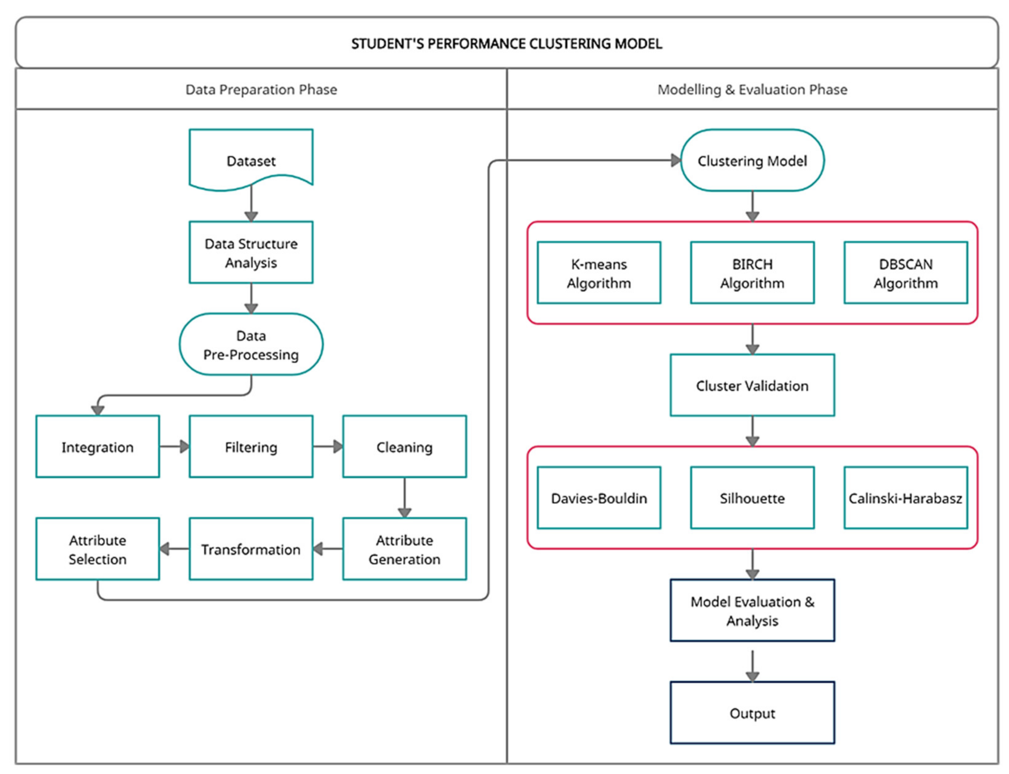
Data Pre-processing. This method focusses on transforming the dataset to ensure it is suitable for the clustering algorithms and the data mining tool. As depicted in Figure 1, six pre-processing techniques are involved: data integration, data filtering, data cleaning, attribute generation, data transformation, and attribute selection. Data integration was carried out at the start of the process, with six source files combined into a single dataset. The dataset was filtered where we only chose Malaysian citizens whose family income attribute ranges from RM 1 to RM 4000, which corresponded to the B40 group. We also consider full-time students for study mode attributes and undergraduate/first-degree students for the level of study attributes. Then, data cleaning was carried out to clear the attributes with too many missing values, such as postcode and parliamentary attributes with more than 30,000 missing values. The attributes that contain some missing values are replaced manually with specified values. Repeated and redundant attributes also have been removed from the dataset. Besides that, two attributes have been generated: registration age based on the date of birth and date of registration, and the number of activities based on the count of student activities. From a total of 53 attributes, only 16 attributes are left, and Table 2 shows the list of the attributes with its description.

Table 2. List of attributes and description.

No.	Attributes	Values	Data Type
1	Gender	Male	Nominal
		Female
2	Registration Age	Below 19	Nominal
		20
		Above 21
3	Marital Status	Single	Nominal
		Married
4	Place of Birth	Northern	Nominal
		Central
		Southern
		East Coast
		East Malaysia and others
5	Income Groups	Below RM2000	Ordinal
		RM2001–3000
		RM3001–4000
6	Secondary School	SMK	Nominal
		SBP and MRSM
		SM Agama
		SM Teknik
		Others
7	Entry Qualification	SPM, STPM and others	Nominal
		Matriculation and foundation programme
		Diploma
8	Sponsorship	Scholarship	Nominal
		Sels-funded
		Loans
9	Residence	Resident	Nominal
		Non-resident
10	University	Research Universities	Nominal
		Comprehensive Universities
		Focussed Universities
11	Field of study	Education	Nominal
		Literature and Humanities
		Social Sciences, Business and Law
		Science, Mathematics and Computer
		Engineering, Manufacturing and Construction
		Agriculture and Vaterinary
		Health and Welfare
		Services
12	CGPA	Below 2.00	Ordinal
		2.01–2.99
		3.00–3.49
		3.50–4.00
13	Industrial Training	None	Nominal
		Pass
		Failed
14	Number of Activities	None	Ordinal
		1
		2
		3 and 4
		5 to 9
		Above 10
15	Employment Status	Working	Nominal
		Unemployed
		Further Study
16	Drop-out Status	Drop-out	Nominal
		Graduate

Most machine learning algorithms generally require numeric input and output variables [32,33,34,35,36,37]. This restriction must be addressed for implementing and developing machine learning models. This implies that all characteristics, including categories or nominal variables, must be transformed into numeric variables before being fed into the clustering and classification model. All these have been dealt with in the data transformation process.

Machine learning models learn how to map input variables to output variables. As a result, the scale and distribution of the domain data may differ for each variable. Input variables may have distinct units, which means they may have different scales. Differences in scaling among input variables may increase the difficulty of the modelled problem. Large input values (for example, a spread of hundreds or thousands of units) can result in a model that learns large weight values. A model with large weight values is frequently unstable, so it may perform poorly during learning and be sensitive to input values, resulting in a larger generalisation error. On top of that, normalization was performed using the StandardScaler or z-transformation and MinMaxScaler methods to form datasets for three different models. The first method, StandardScaler, allows each attribute’s values to be in the same range so that a comparison can be made. Z-transformation normalisation refers to normalising every value in a dataset such that the mean of all values is 0 and the standard deviation is 1 [38]. The equation to perform the z-transformation normalisation on every value in a dataset is as Equation (1), where x_j is the input value of the sample j, $\mu$ is the sample mean, and σ is the standard deviation of the sample data.

$$z_j=\frac{x_j-\mu }{\sigma }$$

(1)

In the second method, MinMaxScaler converts all attributes into a range [0,1], which means the minimum value of the attribute is zero, and the maximum value of the attribute is one [38]. The mathematical formula for MinMaxScaler is defined as Equation (2), where the minimum x_min, and maximum x_max values correspond to the normalised value x.

$$x_j=\frac{x_j-x_{min}}{x_{max}-x_{min}}$$

(2)

Descriptive Analysis.Table 3 shows the descriptive analysis of the student’s dataset after it has been transformed into numerical data. A variable containing categories that lack a natural order or ranking is referred to as a nominal scale. Calculations like a mean, median, or standard deviation would be pointless for nominal variables because they are arbitrary. Hence, Table 3 does not generate the mean, median, or standard deviation for the nominal variables. Descriptive analysis of student’s dataset. Attributes with the highest standard deviations are CGPA and number of activities (0.922 and 1.684, respectively). Besides these two, a huge gap between the other attributes can be observed.

Table 3. Descriptive analysis of student’s dataset.

	Count	Mean	Std	Min	0.25	0.5	0.75	Max
University	117069	-	-	1	1	2	3	-
Registration Age	117069	-	-	1	1	2	2	-
Qualification	117069	1.823	0.739	1	1	2	2	3
Field of Study	117069	-	-	1	3	4	5	-
Sponsorship	117069	-	-	1	2	2	3	-
CGPA	117069	2.764	0.922	1	2	3	3	4
Industrial Training	117069	-	-	0	0	1	1	-
Number of Activities	117069	2.486	1.684	0	1	2	4	5
Employment Status	117069	-	-	1	1	1	2	-
Drop-out Status	117069	0.825	0.38	0	1	1	1	1

Feature Selection. Too many attributes in educational datasets can cause a curse of dimensionality and difficulties when processing and analysing the data. Moreover, calculation of distance by clustering algorithms may not be effective for high-dimensional data. To solve this problem, feature selection methods are applied to find the best attributes for this study. The feature selection methods can be divided into supervised and unsupervised. The features in supervised feature selection methods are chosen based on their relationship to the class label. It chooses qualities that are most relevant to the class label. On the other hand, unsupervised feature selection approaches assess feature relevance by exploring data using an unsupervised learning method [38].

The attributes in the dataset will go through the supervised feature selection process using random forest, extra tree, info gain, and chi-square techniques. After the execution, the attributes have been allocated weights based on their relative importance and are sorted in order. For this experiment, drop-out status has been selected as the class label. The selected attributes which were found to be significant are the place of birth, income groups, secondary school, number of activities, CGPA, employment status, registration age, entry qualification, sponsorship, university, the field of study, and drop-out status.

Then, Kendall’s W statistic is used to assess agreements between all the raters by showing the statistical value between 0 and 1. If the value is “zero”, there is no agreement between the raters, while the value “one” indicates complete agreement. Kendall’s W assessment produced a score of 0.8862 and showed good and strong agreement among all raters used.

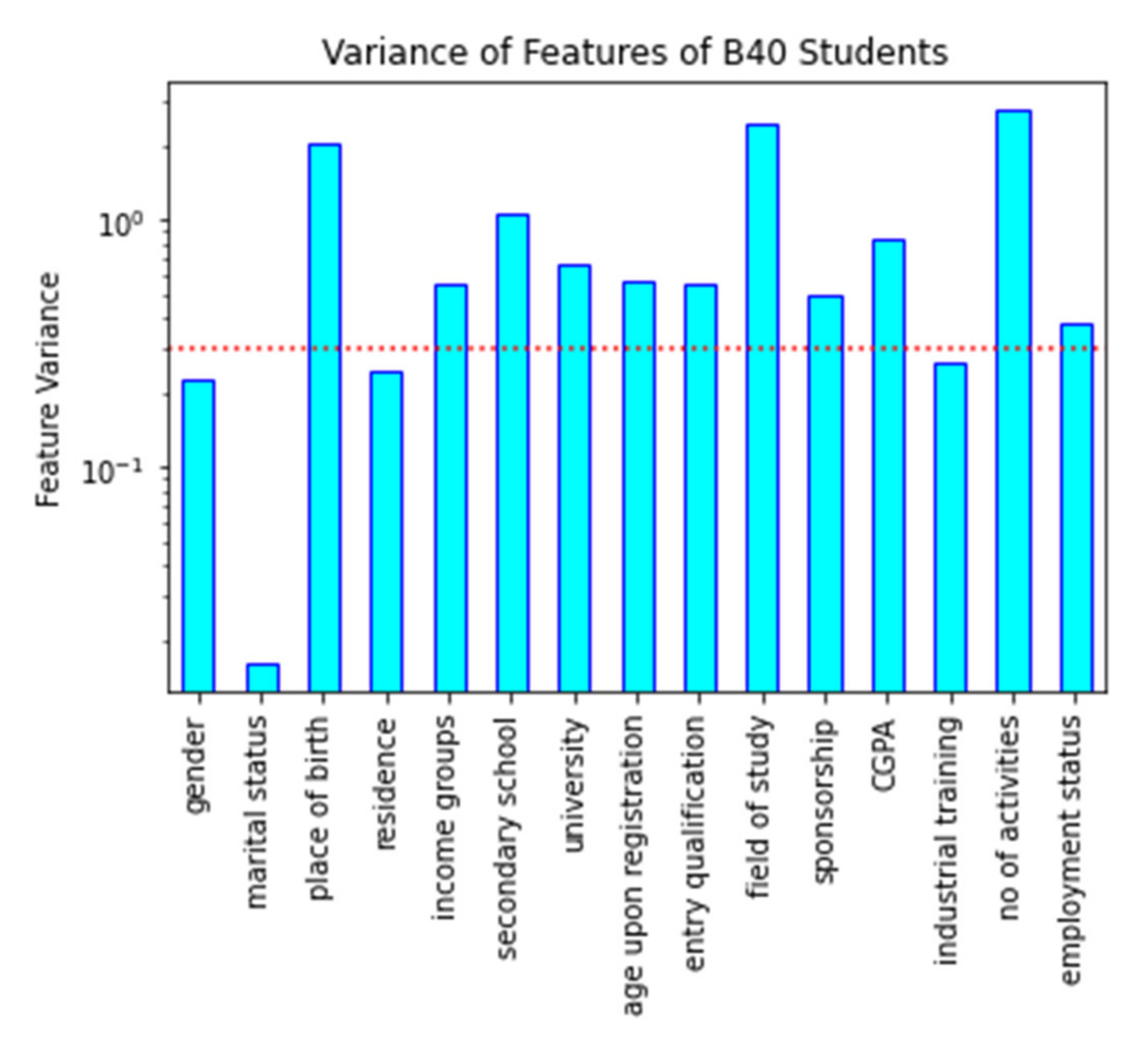
For unsupervised feature selection, a variance threshold will be used on the dataset. Variance is a metric that measures how dispersed the data distribution is within a dataset. Selecting attributes with considerable variance is necessary to avoid developing a biased clustering model and skewed toward certain attributes. Before developing an unsupervised machine learning model, choosing attributes based on their variance is essential. A high variance indicates that the attribute’s value is unique or has a high cardinality. Attributes with low variation have relatively comparable values, but attributes with zero variance have similar values. Furthermore, low-variance attributes are close to the mean value, providing minimal clustering information [8]. Because it solely evaluates the input attribute (x) without considering data from the dependant attribute, the variance thresholding technique is appropriate for unsupervised modelling (y). The variance of all student attributes is shown in Figure 2. As suggested by [39], in this study, the variance threshold value for attribute selection was set to 0.3 to eliminate redundant features with low variance. Based on observations from the figure, there are ten attributes with variance values exceeding 0.3, which indicates that its behavioural patterns are high. The features that have high variance are the place of birth, income groups, secondary school, university, registration age, entry qualification, the field of study, sponsorship, CGPA, number of activities, and employment status. On the other hand, there are four attributes with a variance value of less than 0.3, namely gender, marital status, residence, and industrial training. The attributes of the state of birth, field of study, and the number of activities show the highest variance value and can be used to show student performance patterns.

Figure 2. Variances of the features.

Additionally, gender, marital status, residence, and industrial training attributes are low-variance features. As all three attributes’ marital status has the lowest variance, the other two are close to the threshold, as seen in Figure 2. Furthermore, only 12 attributes with high variance (i.e., place of birth, income groups, secondary school, university, registration age, entry qualification, field of study, sponsorship, CGPA, number of activities, and employment status) are chosen at the end of the unsupervised feature selection, including the drop-out status attribute, and will be used in the next phase.

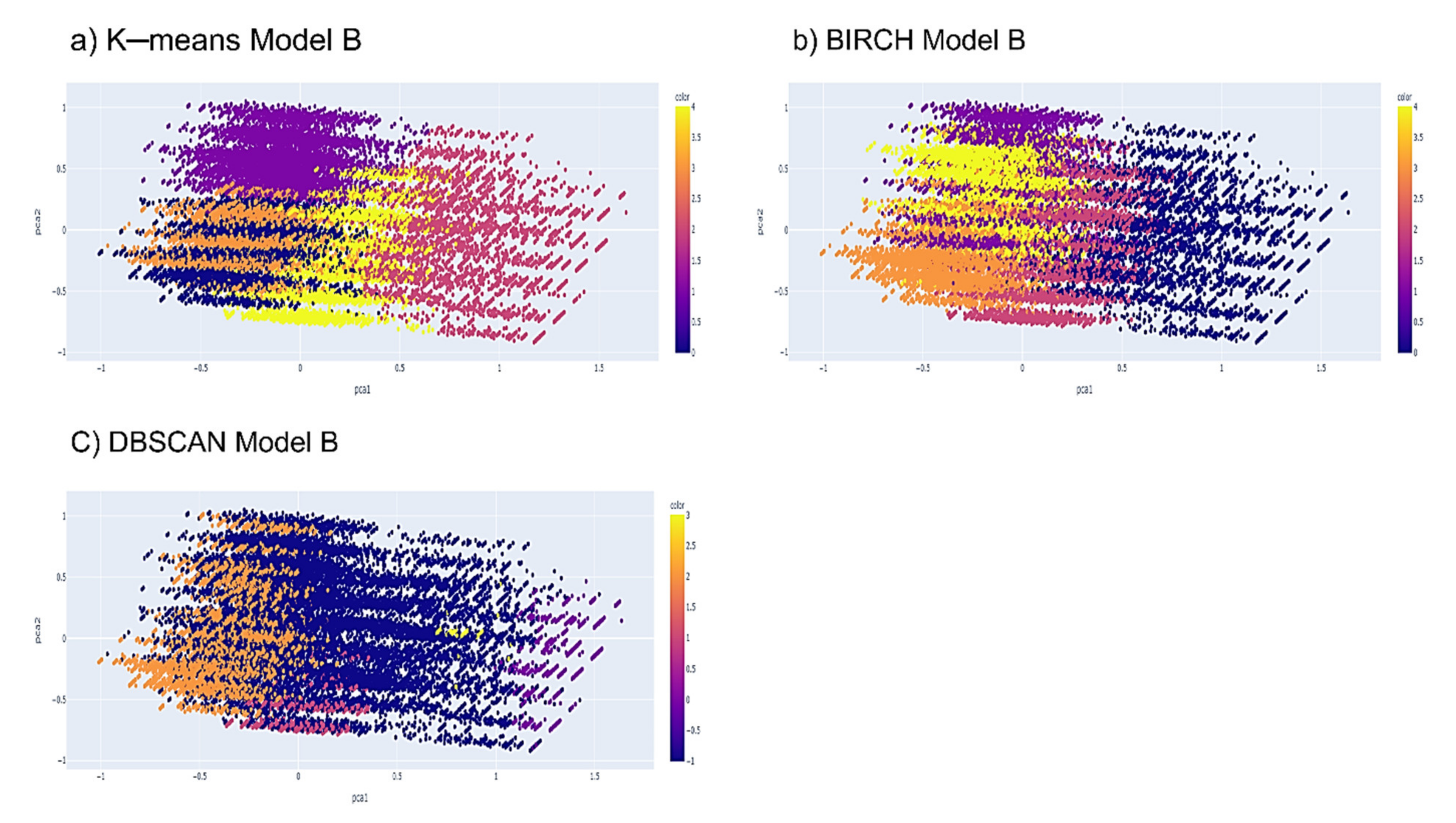
Final Dataset.Table 4, Table 5 and Table 6 show a list of selected sets of attributes after the attribute selection paired with StandardScaler and MinMaxScaler normalization methods. These sets of attributes are named Model A, Model B, and Model C, which will then be the inputs to the clustering models. Model A is a dataset that is normalized with StandardScaler and has 10 attributes after the supervised feature selection. Model B is a dataset that is normalized with MinMaxScaler and has 10 attributes after the supervised feature selection. Lastly, Model C is a dataset that is normalized with MinMaxScaler and has 12 attributes after the unsupervised feature selection.

Table 4. Model A (StandardScaler and supervised feature selection).

No.	Attribute	No.	Attribute
1.	Number of Activities	6.	Qualification
2.	CGPA	7.	Sponsorship
3.	Employment Status	8.	University
4.	Industrial Training	9.	Field of study
5.	Registration Age	10.	Drop-out Status

Table 5. Model B (MinMaxScaler and supervised feature selection).

No.	Attribute	No.	Attribute
1.	Number of Activities	6.	Qualification
2.	CGPA	7.	Sponsorship
3.	Employment Status	8.	University
4.	Industrial Training	9.	Field of study
5.	Registration Age	10.	Drop-out Status

Table 6. Model C (MinMaxScaler and unsupervised feature selection).

No.	Attribute	No.	Attribute
1.	Place of Birth	7.	Registration Age
2.	Income Groups	8.	Qualification
3.	Secondary School	9.	Sponsorship
4.	Number of Activities	10.	University
5.	CGPA	11.	Field of study
6.	Employment Status	12.	Drop-out Status

3.2. Proposed Clustering Methodology

In recent years, the effectiveness of the use of clustering techniques in student performance prediction studies has attracted the interest of many researchers. The clustering technique refers to one method of grouping several similar objects into one cluster while different objects into another. The clustering technique will be very useful if the labelled information from students in the dataset is unknown. In addition, the division of large data sets into small, logical clusters will make it easier for researchers to examine and explain the meaning of the data.

K-means Algorithm. The researchers’ main choice is the k-means algorithm, a popular clustering technique. This technique is popular because the way it is implemented is very simple, and the results are also easy to understand. The k-means algorithm is a method for grouping nearby objects into the k number of the centroid. The elbow method is a popular way to figure out the best number of clusters. When given several clusters, k, this approach calculates the total of the within-cluster variance, also known as inertia, and then shows the variance curve concerning k. The best number of clusters could be the k value at the curve’s initial turning point.

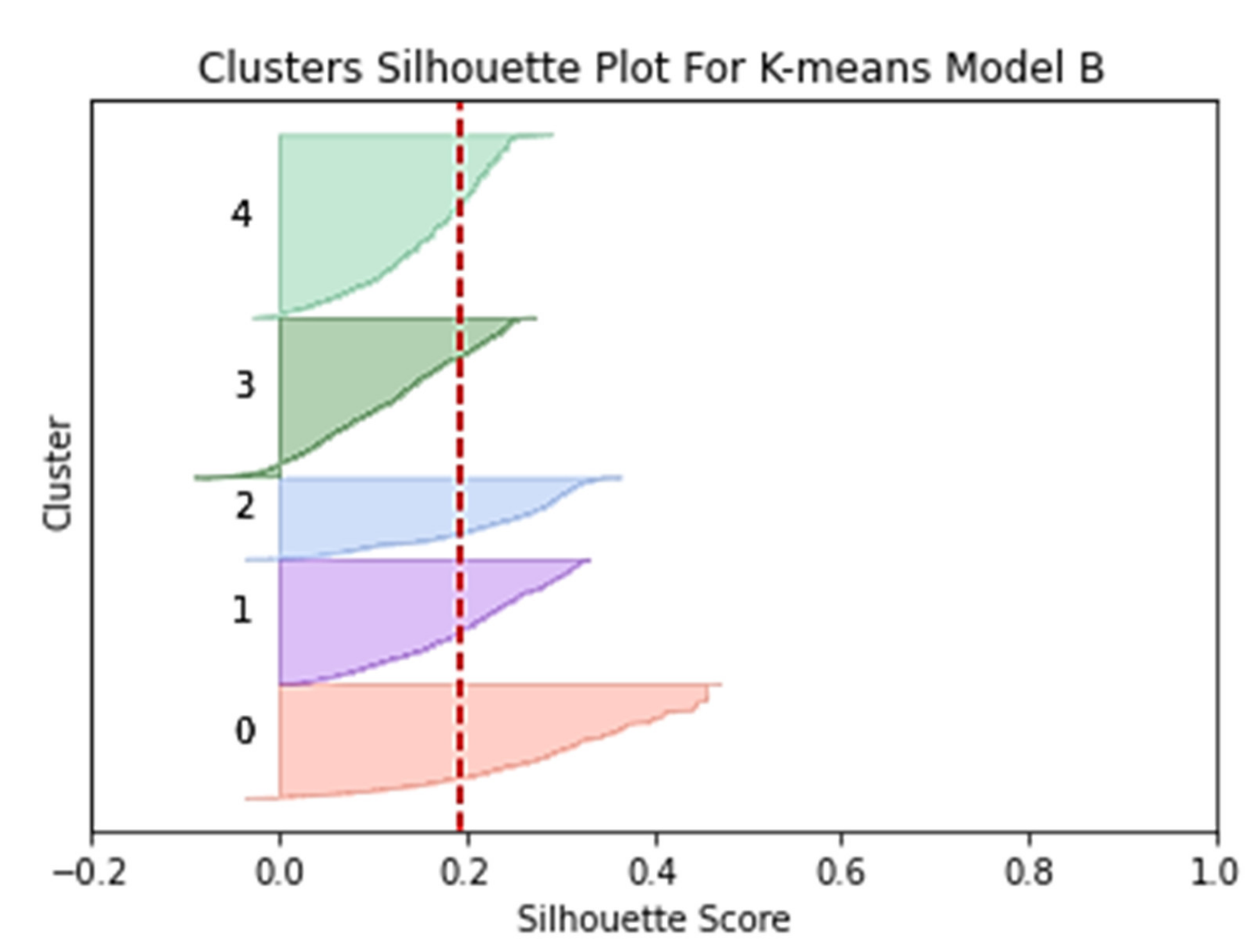
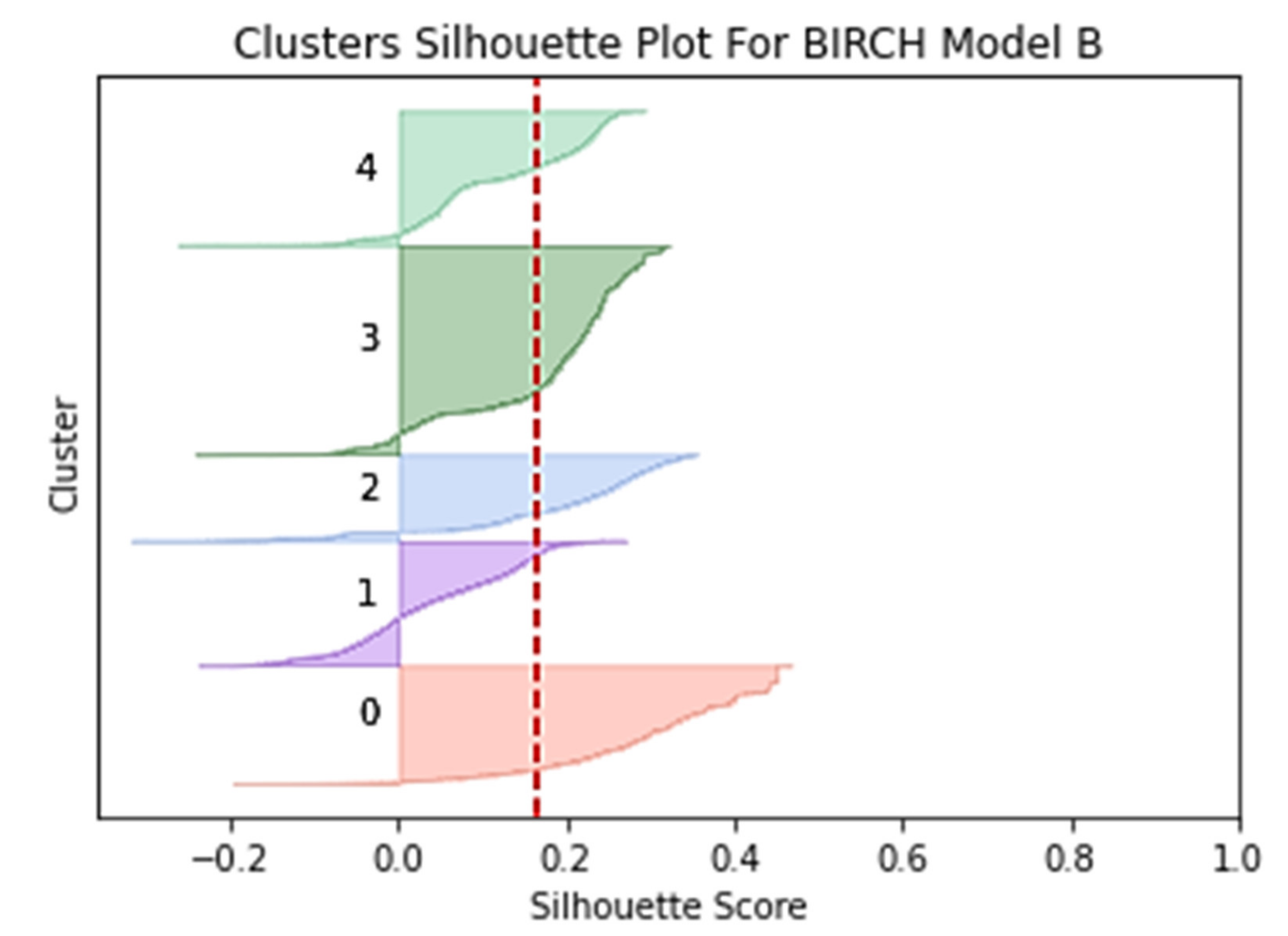
The alternative technique is to use silhouette plot analysis by calculating the coefficients for each data point to measure its similarity with its cluster as compared to other clusters. The value of the silhouette coefficient is in the range [1,−1] where a high value indicates that the object is well matched to its cluster.

BIRCH Algorithm. The BIRCH algorithm is an agglomerate hierarchical clustering technique that excels at huge datasets with high dimensionality. By aggregating the cluster’s zero, first, and second moments, BIRCH generates a height-balanced clustering feature tree of nodes that summarises data. The clustering feature (CF) produced is utilised to determine the centroids and quantify the cluster’s compactness and distance. This storage of statistical information in the CF, such as the number of data points, the linear sum of N points, and the sum of squares of N points, reduces the number of recalculations and allows for incremental sub-cluster merging.

DBSCAN Algorithm. One of the most popular algorithms in the density clustering category is DBSCAN, which was introduced by Martin Ester, Hans-Peter Kriegel, Jorg Sander, and Xiaowei Xu in 1996. This algorithm separates the data points into three parts. The first part is the main point which is the points that are in the cluster. The second part is the boundary points which are the points that fall into the neighbourhood of the main point. The last part is the noise, which is the points not included in the main and boundary points. DBSCAN is very sensitive to the setting of epsilon parameters where a small value will cause the resulting clusters to be categorized as noise. At the same time, the change to a larger value will cause the clusters to be merged and become denser. DBSCAN does not require setting the number of clusters at the start-up phase of the algorithm.

3.3. Parameters Tuning

In machine learning, parameter tuning selects the optimal parameters for a learning algorithm through experimentation. The value of a parameter is utilised to control the learning process. Three clustering algorithms are compared in this study, which are k-means, BIRCH, and DBSCAN. Each algorithm is tuned using different tuning parameters to produce high accuracy results. Its implementation requires the specification of parameters for a specific algorithm, with the tested tuning values shown in Table 7. A number of experiments are carried out using the B40 student dataset to determine the best parameter values for each algorithm. After that, the performance of the three cluster algorithms is reviewed and compared. The optimum parameter tuning values from the experiments for the k-means, BIRCH, and DBSCAN algorithms are used to develop the algorithms in the following experiment to produce high accuracy results. Table 7 shows the final parameters with optimal values. All of the results presented in this research were obtained using the k-means, BIRCH, and DBSCAN algorithms with the optimal tuning value, as shown in Table 7.

Table 7. Results of parameter tuning.

Clustering Model	Parameter	Tested Tuning Value	Optimum Tuning Value
k-means	k	2 to 10	5
	n_iter	5–10 in steps of 1	10
	max_iter	100–500 in steps of 100 Euclidean	300
	Distance metric		Euclidean
BIRCH	n_clusters	2 to 10	5
	threshold	0.1–0.10 in steps of 0.1	0.5
	branching_factor	10–100 in steps of 10	50
DBSCAN	epsilon	0.1–3.0 in steps 0.5	0.5 (Model C) and 1.0 (Model A and B)
	metric	Euclidean	Euclidean
	min_samples	1000–2000 in steps of 20	1000 (Model B and C) and 1200 (Model A)

3.4. Clustering Model Evaluation

In the clustering analysis phase, the accuracy or quality of clustering results will be determined and confirmed. It is an important measurement in determining which algorithm achieved the best performance by using input data for the study. Clustering evaluation is a stand-alone process and is not included during the clustering process. It is always carried out after the final output of the clustering is produced [38]. There are two methods practiced in measuring the quality of clustering results: internal validation and external validation.

Internal validation is the process of evaluating clustering that is compared to the results of the clustering itself, namely the relationship between the structures of clusters that have been formed. This is more realistic and efficient in solving problems involving educational datasets with increasing daily sizes and dimensions.

This study used three types of internal validation methods that are often used in recent clustering studies: (1) the Davies-Bouldin index (DB), (2) the silhouette coefficient index, and (3) the Calinski-Harabasz index (CH). Important notations to be used in mathematical formulas for grouping assessment measurements are as follows: D is the input data set, n is the number of data points in D, g is the midpoint for the entire D data set, P is the dimension number of D, NC is the number of the group, C_i is the i-th group, n_i is the number of data points in C_i, C_i is the midpoint for the C_i group, and d(x,y) is the distance between points x and y [40].

Davies-Bouldin. The Davies-Bouldin (DB) metric is a method that has long been introduced but is still widely used in internal validation measurements. DB uses intra-group variance and inter-group midpoint distance to determine the worst group pairs. Thus, the reduction in DB index value provides the optimum group number. The mathematical formula for DB is defined as Equation (3) [40].

$$DB=\frac{1}{NC}{{\displaystyle \sum }}_i\underset{j\ne i}{\max }\frac{\frac{1}{n_i}{{\displaystyle \sum }}_{x\in C_i}d\left(x,c_i\right)+\frac{1}{n_j}{{\displaystyle \sum }}_{x\in C_j}d\left(x,c_j\right)}{d\left(c_i,c_j\right)}$$

(3)

Silhouette Coefficient Index. The silhouette coefficient index is used to evaluate the quality and strength of a group. The high silhouette coefficient value indicates a model with a better batch and signals that an object is well matched to its batch and does not match the adjacent batches. The equation for calculating the value of the silhouette coefficient of a single sample is as Equation (4):

$$s=\frac{1}{NC}{\displaystyle \sum }_i\left(\frac{1}{n_i}{\displaystyle \sum }_{x\in C_i}\frac{b\left(x\right)-a\left(x\right)}{max\left[b\left(x\right),a\left(x\right)\right]}\right)$$

(4)

where $a\left(x\right)=\frac{1}{n_i-1}{{\displaystyle \sum }}_{y\in C_i,y\ne x}d\left(x,y\right),$ and $b\left(x\right)=mi{n}_{j\ne i}\left[\frac{1}{n_j}{{\displaystyle \sum }}_{y\in C_j}d\left(x,y\right)\right]$.

S does not consider c_i or g and uses pairwise distances between all objects in the clusters to calculate the density a(x). At the same time, b(x) measures separation, the average distance of objects to alternative groups or the nearest second group. Of Equation (2), the silhouette coefficient values range can be between −1 and 1. The greater the positive value of the coefficient, the higher the probability of it being grouped in the right cluster. In contrast, elements with negative coefficient values are more likely to be grouped in the wrong cluster [41,42].

Calinski-Harabasz Index. The Calinski-Harabasz (CH) index measures two criteria simultaneously using the average power-added result between two groups and the average yield of two plus forces in the group. The numerator in the formula describes the degree of separation, the extent to which the midpoint of the group is scattered. The denominator also describes the density that is as close as the objects in the group gather around the midpoint. The mathematical formula for CH is defined as Equation (5):

$$CH=\frac{{{\displaystyle \sum }}_i{d}^2\left(c_i,g\right)/\left(NC-1\right)}{{{\displaystyle \sum }}_i{{\displaystyle \sum }}_{x\in C_i}{d}^2\left(x,c_i\right)/\left(n-NC\right)}$$

(5)

4. Experimental Results and Analysis

4.1. Internal Validation

This section demonstrates the clustering results obtained using the proposed method. Indicators that should be given attention when checking the scores of clustering evaluation metrics are as follows: low DB index values; silhouette coefficient index with a high positive value; and the CH index with high values shows good clustering achievement. Table 8 summarizes the results of clustering performance based on internal validation for three clustering algorithms, k-means, BIRCH, and DBSCAN, applied to three different model types: Model A, Model B, and Model C. The algorithm’s running time to execute is also given in the table.

Table 8. Result of clustering model evaluation.

Algorithm	Model A				Model B				Model C
	DB	Silhouette	CH	Time (s)	DB	Silhouette	CH	Time (s)	DB	Silhouette	CH	Time (s)
k-means	1.85	0.18	20,846.33	238	1.71	0.192	24,946.34	238	1.891	0.16	17,358.46	231
BIRCH	2.08	0.14	17,203.63	254	1.96	0.165	21,722.28	223	2.222	0.12	14,664.02	235
DBSCAN	1.43	−0.17	3034.38	269	2.08	0.082	11,218.19	306	2.229	−0.02	6760.80	308

Table 9 summarizes clustering performance based on the internal validation of three clustering algorithms, k-means, BIRCH, and DBSCAN, applied to three models: Model A, Model B, and Model C. The internal validation evaluation metrics used in this study show if the clusters produced are well separated and if data points do not overlap.

Table 9. Final score ranking based on the algorithms.

Algorithm	Model A				Model B				Model C
	DB	Silhouette	CH	Mean Score	DB	Silhouette	CH	Mean Score	DB	Silhouette	CH	Mean Score
k-means	2	2	2	2	1	1	1	1	3	3	3	3
BIRCH	2	2	2	2	1	1	1	1	3	3	3	3
DBSCAN	1	1	3	2	2	2	1	2	3	3	2	3
Total mean score	6				4				9
Ranking position	2				1				3

Based on the results of clustering performance in Table 8, each algorithm is ranked to identify its performance. Table 9 shows the list of ranks for each algorithm based on the mean score of DB, silhouette, and CH. For example, the k-means algorithm for Model B is given the first rank because after comparing it with other models, its DB has the lowest value, the silhouette has the highest value, and the CH has the highest value. Model B recorded the best mean score of 4, followed by Model A with a score of 6 and Model C with a total score of 8. Hence, Model B is the best model compared to the other two based on the table above.

From the comparison between all of the models above, we will focus on the evaluation analysis of the three clustering algorithms used in Model B because it was better than Model A and C. Table 8 shows the DB index, silhouette coefficient index, and CH index clearly show the k-means dominance over the other two algorithms. The DB index value for the k-means is 1.71, which is lower than BIRCH (1.96) and DBSCAN (2.08). For the silhouette index, k-means again recorded the best result where the value is the highest (0.192) as compared to BIRCH (0.165) and DBSCAN (0.082). Meanwhile, for the CH index, values recorded by all three algorithms are 24946.34 for k-means, the highest, followed by 21722.28 for BIRCH and 11218.19 for DBSCAN. So, based on the internal validation evaluation, the k-means algorithm was the best for Model B.

4.2. Silhouette Analysis

Additional analysis to investigate the clustering results of the k-means and BIRCH algorithms is examining the silhouette plots as in Figure 3 and Figure 4. The plot in Figure 3 shows that all five clusters generated by the k-means are above the silhouette average value line, giving a good picture of the clustering results. The mean value of the Model B silhouette coefficient index for the K-means (KMoB) is 0.192 and is marked on the plot with a red dotted line. The fluctuation of the silhouette plot size did not show a significant change where all clusters recorded a positive mean score, indicating that almost all values were assigned to the correct cluster.

Figure 3. Clusters silhouette plot for k-means Model B (KMoB).

Figure 4. Clusters silhouette plot for BIRCH Model B.

The silhouette plot in Figure 4 shows that all five clusters generated by the BIRCH algorithm are above the silhouette average value line and show good clustering results. The mean value of the Model B silhouette coefficient index for the BIRCH algorithm is 0.165 and is shown on the plot with a red dotted line. Compared to the k-means, the silhouette coefficient value of the BIRCH algorithm decreased by 0.027. Plot size fluctuations showed large and significant changes where small sizes were indicated by clusters 1, 2, and 4 while large sizes were indicated by clusters 0 and 3.

4.3. Visualization of The Clustering Results

Based on the internal validation evaluation metrics discussions, the results clearly show why the k-means technique performs better than BIRCH and DBSCAN in Model B. To further explain the clustering results, we have taken the principal component analysis method (PCA) approach to reduce the dimensions of student attributes to two-dimensional spaces. The two principal components were then plotted on a scatter chart to produce visual clustering results as in the study [8]. In Figure 5, three plots of different algorithms are shown whereby five different colours symbolize five different clusters.

Figure 5. Clustering results of Model B using (a) k-means (KMoB); (b) BIRCH; (c) DBSCAN.

The separation method between clusters in Model B is the best because the clusters separated from each other are distinguished by colours. By comparison, the k-means algorithm for Model B (KMoB) produced the best clusters, followed by the BIRCH algorithm and the DBSCAN algorithm. The result of the DBSCAN algorithm is the weakest because it cannot separate the data points properly, and extreme overlap can be observed in the plot. Apparently, the noise samples make the clusters less represenYestative in all plots.

4.4. Feature Extraction

Further analysis was conducted on the extraction of features from the k-means Model B (KMoB). Table 10 shows the KMoB’s clustering results by listing each cluster’s important attributes. Notably, for the drop-out status attribute, the graduate (1) value affects clusters 0, 1, 3, and 4, with the highest percentage of students falling in cluster 0 (27.48%). While the drop-out (0) only affected cluster 2, accounting for 18.8% of students (refer to Figure 6).

Table 10. Descriptive statistics from the clustering result for the KMoB.

Attribute	Cluster 0	Cluster 1	Cluster 2	Cluster 3	Cluster 4
Drop-out Status	Graduate	Graduate	Drop-out	Graduate	Graduate
%	27.48	23.99	17.21	18.71	12.28
CGPA	3.01–3.49	3.01–3.49	Below 2.00	3.01–3.49	3.01–3.49
%	12.78	12.39	10.57	8.99	5.64
Employment Status	Working	Working	Unemployed	Working	Working
%	17.34	14.59	17.2	12.78	8.23
No. of Activities	Above 10	5 to 9	None	1	1
%	8.04	5.6	13.33	6.16	2.92
Field of Study	Social Sciences, Business, and Law	Engineering, Manufacturing, and Construction	Engineering, Manufacturing, and Construction	Engineering, Manufacturing, and Construction	Engineering, Manufacturing, and Construction
%	12.12	7.57	6.37	7.18	4.6
Qualification	SPM, STPM, and others	Matriculation and foundation programme	Diploma	Matriculation and foundation programme	Diploma
%	24.08	15.62	8.96	17.77	10.92
Industrial Training	Pass	Pass	Failed	Pass	Pass
%	16.76	13.8	16.57	14.41	7.41
Sponsorship	Loans	Self-funded	Self-funded	Loans	Loans
%	19.31	8.75	10.25	11.43	6.3
Registration Age	20	Below 19	Above 21	Below 19	Above 21
%	25.48	12.02	10.12	17.5	11.98
University	Focussed	Research	Comprehensive	Focussed	Focussed
%	16.93	18.82	7.99	14.52	7.19
Cluster Size	32,315	28,206	22,005	20,145	14,398
%	27.6	24.09	18.8	17.21	12.3

Figure 6. Clustering result of students’ drop-out status.

The CGPA attribute with a value of 3.01–3.49 was a distinct characteristic for clusters 0, 1, 3, and 4, where the highest percentage of students (12.78%) is in cluster 0. Only cluster 2 has recorded a CGPA value of below 2.00 for 10.57% of students (refer to Figure 7). Working as a distinct value in clusters 0, 1, 3, and 4, with the highest percentage of students belonging to cluster 0. Cluster 2 comprises unemployed students who recorded a percentage of 17.2%. Next, the number of “1” activities affected clusters 3 and 4, accounting for 6.16 and 2.92 per cent of the total students, respectively. The value “5–9” affected only cluster 1, accounting for 5.6%, while the value “above 10” affected only cluster 0, accounting for 8.04%. Cluster 2 recorded the “none” value, accounting for 13.33% of the total number of students.

Figure 7. Clustering results of students’ CGPA.

For the field of study, “engineering, manufacturing, and construction” have been observed as the majority in clusters 1, 2, 3, and 4, with cluster 1 having the largest percentage of students at 7.57%. While the field of “social sciences, business, and legislation” are only observed in cluster 1 with a percentage of 12.12% of students. Qualification for the university entrance for cluster 1 is SPM, STPM, and others, accounting for 24.08% of the total students. While clusters 1 and 3 were influenced by matriculation and foundation, with percentages as high as 15.62% and 17.77%, respectively.

The last two clusters of 4 and 2 were influenced by diplomas with 10.92% and 8.96%, respectively. Industrial training attributes showed that the students who passed had influenced four clusters, with cluster 0 recording the highest percentage, followed by clusters 3, 1, and 4. While cluster 2 was influenced by the failed results amounting to 16.57% of total students. Besides that, three clusters were dominated by study loans, and they are clusters 0, 3, and 4, with the highest percentage recorded by cluster 0. Self-funded students were the majority in clusters 2 and 1, with percentages as high as 10.25% and 8.75% each.

Registration age attribute shows that values under 19 affected clusters 3 and 1 with 17.5% and 12.02% percentages, respectively. Cluster 0 became the only cluster affected by the value “20” with 25.48%. The percentage of students belonging to clusters 4 and 2 that were influenced by students older than 21 was 11.98% and 10.12%, respectively. The last attribute is university and observations, and it is found that cluster 1 was influenced by research universities with a percentage as high as 18.82%. Comprehensive universities, on the other hand, only influenced cluster 2 by 7.99%. In contrast, focused universities become an influential value with three clusters involved. Those clusters were 0, 3, and 4, with 16.93%, 14.52%, and 7.19% of the total B40 students.

4.5. Class Label

Based on the previous analysis, we can conclude that the clustering results can establish five class labels: the highest, highest, medium, low, and lowest performance groups. Table 11 summarizes the cluster’s class label based on the student’s performance.

Table 11. Clusters class labels based on the student’s performance.

Cluster	Class Label	No. of Students
0	Highest	32,315
1	High	28,206
2	Lowest	20,145
3	Medium	22,005
4	Low	14,398

Cluster 0 represents the group with the highest performing students who received a high CGPA, recorded a high number of participation in activities, and had a high employment rate after graduation. While cluster 2 represents the lowest performing students with low CGPA in their studies, fewer participation in activities at university, students who failed to get employed after graduation, and a high number of drop-out cases. Clusters 1, 3, and 4 represent students with high, moderate, and low performance, where their CGPA, number of participation in activities, employment status after graduation, and successful graduation status are in between group 0 and group 2 achievements.

4.6. Classification Model on Student’s Performance

After the KMoB determined five class labels, the cluster dataset was used to develop the B40 student performance, classification model. The development of this classification model aims to select the best model that can classify B40 students based on performance class labels that have been produced. Performance of the models that have been used, such as decision tree, random forest, and artificial neural network (ANN), are reported in Table 12. In terms of classification accuracy, all three algorithms produced high accuracy values, and the differences are not very significant. The ANN algorithm recorded the highest accuracy of 99.92%, followed by random forest at 99.81%. The lowest accuracy was produced by the decision tree algorithm or J48, which is 99.71%.

Table 12. Performance results of the classification models.

Classifier	Accuracy (%)
Decision tree	99.71
Random forests	99.81
ANN	99.92
Average	99.81

A statistical test has been conducted to determine if the performance produced by one classifier is better than the other. The selected statistical test is a paired t-test for classification performance with a confidence level of 0.05 (95%).

Based on Table 13, the ANN marked with (1) is the base comparison with an accuracy value of 99.92%. The ANN accuracy was compared to random forests marked with (2) and decision trees marked with (3). The test results showed the asterisk symbol (*) in random forests and decision trees that indicated the accuracy of these two classifiers was significantly lower than the ANN. This means ANN is the best classifier, and the paired t-test shows the results are statistically significant at a confidence level of 0.05.

Table 13. Classification performance t-test result.

Test: Paired t-test
Analysis: Percentage of correctly classified
Dataset: k-means Model B
Confidence: 0.05 (two tailed)
Data label	(1) ANN	(2) Random forests	(3) Decision tree
k-means Model B	99.92	99.81 *	99.71 *
	(v/ /*)	(0/0/1)	(0/0/1)

* Indicates that the result is different from the ANN.

5. Discussion

The k-means algorithm produces the best clustering compared to the BIRCH and DBSCAN algorithms. This is due to k-means algorithms that easily cluster high-dimensional numerical data. Implementing k-means also helped label groups of students and successfully selected influential features in this student dataset. In general, the k-means algorithm is reliable and consistently produces consistent clusters after several runs of tests.

The BIRCH algorithm, the second-best algorithm for Model B, has produced low classification quality compared to k-means. After the analysis was conducted, it was found that the characteristics of the students were not well separated. This weakness may be related to the lack of this algorithm, which is sensitive to the arrangement of records in the data set and prefers spherical clusters.

Moreover, the evaluation results show that DBSCAN is the lowest and weakest algorithm in clustering student datasets. The clustering analysis results also showed that the students could not be separated well, and there were no prominent performance characteristics for each group of students. The DBSCAN algorithm is a density-based clustering technique that assumes that clusters are high-density areas in a single space and are separated by low-density areas. So, this algorithm can identify clusters in a dataset by simply looking at the local density of data points. In this case, the DBSCAN algorithm cannot cluster well because the student dataset used is both high-dimensional and not spatial in nature, with noise causing the complexity to be high [40]. The principal component analysis method (PCA) approach successfully reduced the dataset’s dimensions but caused data interpretation difficulties.

6. Conclusions

This paper proposed an unsupervised clustering framework for classifying B40 students’ performance using k-means, BIRCH, and DBSCAN algorithms. The dataset used in this study has 117,069 undergraduate students’ information with 16 attributes from 20 public HEIs. The experimental results demonstrate that three clustering models have been successfully developed using k-means, BIRCH, and DBCSCAN algorithms. Then, the analysis showed that the k-means algorithm applied to Model B (KMoB) produced the best performance when compared to the other two models. Attributes such as CGPA, number of activities, employment status, and drop-out status were the most important attributes in classifying students’ performance. The cluster labels, which are the output of the methods, can be produced and distinguished by these four important attributes. Next, a B40 students performance classification model was developed using the k-means Model B cluster dataset that included class labels generated by the KMoB. The experimental results show that the ANN classification algorithm has produced the best model with accuracy performance as high as 99.92%. Based on the study, the management of Malaysian public HEIs can use the KMoB to cluster the B40 student based on their performance in higher education institutions to reduce drop-out rates as this model can identify student performance levels during their studies. With these students’ early detection abilities, intensive and effective early interventions can be carried out to support and guide students to master the lessons well. For better clustering analysis of students’ dataset, future work should include the following: (1) expand the dataset by adding more attributes related to student performance, behavioural, psychological and employment; (2) further improvements of the clustering performance by using suitable feature selection techniques and different parameter tuning.

References

- Ahuja, R.; Jha, A.; Maurya, R.; Srivastava, R. Analysis of Educational Data Mining. In Harmony Search and Nature Inspired Optimization Algorithms; Springer: Singapore, 2019; pp. 897–907. [Google Scholar] [CrossRef]
- Vahdat, M.; Oneto, L.; Ghio, A.; Anguita, D.; Funk, M.; Rauterberg, M. Advances in Learning Analytics and Educational Data Mining. In Proceedings of the 23rd ESANN 2015, Bruges, Belgium, 22–24 April 2015; pp. 297–306. [Google Scholar]
- Sani, N.S.; Nafuri, A.F.M.; Othman, Z.A.; Nazri, M.Z.A.; Mohamad, K.N. Drop-out Prediction in Higher Education among B40 Students. Int. J. Adv. Comput. Sci. Appl. 2020, 11, 550–559. [Google Scholar] [CrossRef]
- Šarić-Grgić, I.; Grubišić, A.; Šerić, L.; Robinson, T.J. Student Clustering Based on Learning Behavior Data in the Intelligent Tutoring System. Int. J. Distance Educ. Technol. 2020, 18, 73–89. [Google Scholar] [CrossRef]
- Hooshyassr, D.; Pedaste, M.; Yang, Y. Mining Educational Data to Predict Students’ Performance through Procrastination Behavior. Entropy 2019, 22, 12. [Google Scholar] [CrossRef] [PubMed]
- Navarro, Á.A.M.; Ger, P.M. Comparison of Clustering Algorithms for Learning Analytics with Educational Datasets. IJIMAI 2018, 5, 9–16. [Google Scholar] [CrossRef]
- DeFreitas, K.; Bernard, M. Comparative Performance Analysis of Clustering Techniques in Educational Data Mining. IADIS Int. J. Comput. Sci. Inf. Syst. 2015, 10, 65–78. [Google Scholar]
- Li, X.; Zhang, Y.; Cheng, H.; Zhou, F.; Yin, B. An Unsupervised Ensemble Clustering Approach for the Analysis of Student Behavioral Patterns. IEEE Access 2021, 9, 7076–7091. [Google Scholar] [CrossRef]
- Valarmathy, N.; Krishnaveni, S. Performance Evaluation and Comparison of Clustering Algorithms Used in Educational Data Mining. Int. J. Recent Technol. Eng. 2019, 7, 103–112. [Google Scholar]
- Križanić, S. Educational Data Mining Using Cluster Analysis and Decision Tree Technique: A Case Study. Int. J. Eng. Bus. Manag. 2020, 12, 1847979020908675. [Google Scholar] [CrossRef]
- Vital, T.P.; Lakshmi, B.G.; Rekha, H.S.; DhanaLakshmi, M. Student Performance Analysis with Using Statistical and Cluster Studies. In Soft Computing in Data Analytics; Nayak, J., Abraham, A., Krishna, B.M., Chandra Sekhar, G.T., Das, A.K., Eds.; Springer: Singapore, 2019; pp. 743–757. [Google Scholar] [CrossRef]
- Govindasamy, K.; Velmurugan, T. Analysis of Student Academic Performance Using Clustering Techniques. Int. J. Pure Appl. Math. 2018, 119, 309–323. [Google Scholar]
- Prabha, T.; Priyaa, D.S. Knowledge Discovery of the Students Academic Performance in Higher Education Using Intuitionistic Fuzzy Based Clustering. J. Theor. Appl. Inf. Technol. 2017, 95, 7005–7019. [Google Scholar]
- Nafis, M.; Owais, S.T. Students Academic Performance Using Partitioning Clustering Algorithms. Int. J. Adv. Res. Comput. Sci. 2017, 8, 640–644. [Google Scholar] [CrossRef]
- Aldowah, H.; Al-Samarraie, H.; Fauzy, W.M. Educational data mining and learning analytics for 21st century higher education: A review and synthesis. Telemat. Inform. 2019, 37, 13–49. [Google Scholar] [CrossRef]
- Hafzan, M.Y.N.N.; Safaai, D.; Asiah, M.; Saberi, M.M.; Syuhaida, S.S. Review on Predictive Modelling Techniques for Identifying Students at Risk in University Environment. In Proceedings of the 9th EASN International Conference on “Innovation in Aviation & Space”, MATEC Web Conference, Athens, Greece, 3–6 September 2019; Volume 255, pp. 1–8. [Google Scholar] [CrossRef]
- Xu, J.; Moon, K.H.; van der Schaar, M. A Machine Learning Approach for Tracking and Predicting Student Performance in Degree Programs. IEEE J. Sel. Top. Signal Process. 2017, 11, 742–753. [Google Scholar] [CrossRef]
- Márquez-Vera, C.; Cano, A.; Romero, C.; Noaman, A.Y.M.; Fardoun, M.H.; Ventura, S. Early Drop-out Prediction Using Data Mining: A Case Study with High School Students. Expert Syst. 2016, 33, 107–124. [Google Scholar] [CrossRef]
- Statistics of Higher Education. Ministry of Higher Education. Available online: https://www.mohe.gov.my/muat-turun/statistik/2020/493-statistik-pendidikan-tinggi-2020-04-bab-2-universiti-awam/file (accessed on 12 May 2022).
- Palani, K.; Stynes, P.; Pathak, P. Clustering Techniques to Identify Low-Engagement Student Levels. In Proceedings of the 13th International Conference on Computer Supported Education, Online, 23–25 April 2021; pp. 248–257. [Google Scholar]
- Al-Hagery, M.A.; Alzaid, M.A.; Alharbi, T.S.; Alhanaya, M.A. Data Mining Methods for Detecting the Most Significant Factors Affecting Students’ Performance. Int. J. Inf. Technol. Comput. Sci. 2020, 12, 1–13. [Google Scholar] [CrossRef]
- Mallik, P.; Roy, C.; Maheshwari, E.; Pandey, M.; Rautray, S. Analyzing Student Performance Using Data Mining. In Ambient Communications and Computer Systems; Hu, Y.-C., Tiwari, S., Mishra, K.K., Trivedi, M.C., Eds.; Springer: Singapore, 2019; pp. 307–318. [Google Scholar] [CrossRef]
- Francis, B.K.; Babu, S.S. Predicting Academic Performance of Students Using a Hybrid Data Mining Approach. J. Med. Syst. 2019, 43, 162. [Google Scholar] [CrossRef]
- Macedo, M.; Santana, C.; Siqueira, H.; Rodrigues, R.L.; Ramos, J.L.C.; Silva, J.C.S.; Maciel, A.M.A.; Bastos-Filho, C.J.A. Investigation of College Dropout with the Fuzzy C-Means Algorithm. In Proceedings of the IEEE 19th International Conference on Advanced Learning Technologies (ICALT), Maceió, Brazil, 15–18 July 2019; Volume 2161-377X, pp. 187–189. [Google Scholar] [CrossRef]
- Alzahrani, N.A.; Abdullah, M.A. Student Engagement Effectiveness in E-Learning System. Biosc. Biotech. Res. Comm. 2019, 12, 208–218. [Google Scholar] [CrossRef]
- Hussain, M.; Zhu, W.; Zhang, W.; Abidi, S.M.R. Student Engagement Predictions in an E-Learning System and Their Impact on Student Course Assessment Scores. Comput. Intell. Neurosci. 2018, 2018, 6347186. [Google Scholar] [CrossRef]
- Sangodiah, A.; Balakrishnan, B. Holistic Prediction of Student Attrition in Higher Learning Institutions in Malaysia Using Support Vector Machine Model. Int. J. Res. Stud. Comput. Sci. Eng. 2014, 1, 29–35. [Google Scholar]
- Rashid, S.M.R.A.; Samat, N. Kemiskinan Keluarga Dan Pengaruhnya Terhadap Tahap Pendidikan Rendah Masyarakat Luar Bandar: Kajian Kes Di Jajahan Bachok, Kelantan. J. Soc. Sci. Humanit. 2018, 13, 11–23. [Google Scholar]
- Perez, B.; Castellanos, C.; Correal, D. Applying Data Mining Techniques to Predict Student Dropout: A Case Study. In Proceedings of the 2018 IEEE 1st Colombian Conference on Applications in Computational Intelligence (ColCACI), Medellin, Colombia, 16–18 May 2018; pp. 1–6. [Google Scholar] [CrossRef]
- Fredricks, J.A.; Blumenfeld, P.C.; Paris, A.H. School Engagement: Potential of the Concept, State of the Evidence. Rev. Educ. Res. 2004, 74, 59–109. [Google Scholar] [CrossRef]
- Yusuf, N.Y.; Yunus, A.S.M. Tingkah Laku, Emosi Dan Kognitif Murid Sebagai Faktor Peramal Pencapaian Akademik. J. Hum. Cap. Dev. 2014, 7, 1–20. [Google Scholar]
- Nasif, A.; Othman, Z.A.; Sani, N.S. The Deep Learning Solutions on Lossless Compression Methods for Alleviating Data Load on IoT Nodes in Smart Cities. Sensors 2021, 21, 4223. [Google Scholar] [CrossRef] [PubMed]
- Holliday, J.D.; Sani, N.; Willett, P. Calculation of substructural analysis weights using a genetic algorithm. J. Chem. Inf. Model. 2015, 55, 214–221. [Google Scholar] [CrossRef] [PubMed]
- Holliday, J.; Sani, N.; Willett, P. Ligand-Based Virtual Screening Using a Genetic Algorithm with Data Fusion. Match Commun. Math. Comput. Chem. 2018, 80, 623–638. [Google Scholar]
- Bakar, A.A.; Hamdan, R.; Sani, N.S. Ensemble Learning for Multidimensional Poverty Classification. Sains Malays. 2020, 49, 447–459. [Google Scholar] [CrossRef]
- Mansor, N.; Sani, N.S.; Aliff, M. Machine Learning for Predicting Employee Attrition. Int. J. Adv. Comput. Sci. Appl. 2021, 12, 435–445. [Google Scholar] [CrossRef]
- Othman, Z.A.; Bakar, A.A.; Sani, N.S.; Sallim, J. Household Overspending Model Amongst B40, M40 and T20 Using Classification Algorithm. Int. J. Adv. Comput. Sci. Appl. 2020, 11, 392–399. [Google Scholar] [CrossRef]
- Rahman, A.M.; Sani, N.S.; Hamdan, R.; Ali Othman, Z.; Abu Bakar, A. A Clustering Approach to Identify Multidimensional Poverty Indicators for the Bottom 40 Percent Group. PLoS ONE 2021, 16, e0255312. [Google Scholar] [CrossRef]
- Gaurav, M. The Most Comprehensive Guide to Automated Feature Selection Methods in Python. Available online: https://datagraphi.com/blog/post/2019/9/23/feature-selection-with-sklearn-in-python (accessed on 5 June 2022).
- Hassani, M.; Seidl, T. Using Internal Evaluation Measures to Validate the Quality of Diverse Stream Clustering Algorithms. Vietnam J. Comput. Sci. 2017, 4, 171–183. [Google Scholar] [CrossRef]
- Shutaywi, M.; Kachouie, N.N. Silhouette Analysis for Performance Evaluation in Machine Learning with Applications to Clustering. Entropy 2021, 23, 759. [Google Scholar] [CrossRef] [PubMed]
- Lai, D.T.C.; Malik, O.A. A Cluster Analysis of Population Based Cancer Registry in Brunei Darussalam: An Exploratory. Asia-Pac. J. Inf. Technol. Multimed. 2022, 11, 54–64. [Google Scholar] [CrossRef]
Publisher’s Note: MDPI stays neutral with regard to jurisdictional claims in published maps and institutional affiliations. |
© 2022 by the authors. Licensee MDPI, Basel, Switzerland. This article is an open access article distributed under the terms and conditions of the Creative Commons Attribution (CC BY) license (https://creativecommons.org/licenses/by/4.0/).