Abstract
The repeated updating of parametric designs is computationally challenging, especially for large-scale multi-physics models. This work is focused on proposing an efficient modal modification method for gradient-based topology optimization of thermoelastic structures, which is essential when dealing with their complex eigenproblems and global sensitivity analysis for a huge number of design parameters. The degrees of freedom of the governing equation of thermoelastic structures is very huge when its parametric partial differential equation is discretized using the numerical technique. A Krylov subspace preconditioner is constructed based on the Neumann series expansion series so that the thermoelastic eigenproblem can be solved in an efficient low-dimension solver, rather than its original high-fidelity solver. In the construction of Krylov reduced-basis vectors, the computational cost of the systemic matrix inverse becomes a critical issue, which is solved efficiently by means of constructing a diagonal systemic matrix with the lumped mass and heat generation submatrices. Then, the reduced-basis preconditioner can provide an efficient optimal solver for both the thermoelastic eigenproblem and its eigen sensitivity. Furthermore, a master-slave pattern parallel method is developed to reduce the computational time of computing the global sensitivity numbers, and therefore, the global sensitivity problem can be efficiently discretized into element-scale problems in a parallel way. The sensitivity numbers can thus be solved at the element scale and aggregated to the global sensitivity number. Finally, two case studies of the iterative topology optimization process, in which the proposed modal modification method and the traditional method are implemented, are used to illustrate the effectiveness of the proposed method. Numerical examples show that the proposed method can reduce the computational cost remarkably with acceptable accuracy.
1. Introduction
The repeated updating of parametric designs is computationally challenging, especially for large-scale multi-physics models. Thermoelastic structures are involved in many engineering fields. For example, micro-electronic mechanical systems with thermodynamic behavior now dominate the billion-level market, including aviation, space, and daily life [1]. Thermoelastically coupled microresonators are usually used as the core component of micro-electronic mechanical systems and have two main characteristics: the resonant frequency and dissipative ratio [2,3,4]. A higher resonant frequency leads to a higher reaction speed and sensitivity, while a lower dissipative ratio means better accuracy. There are dense analyses of the characteristics of thermoelastically coupled microresonators, including analytical, numerical, and experimental analyses of the resonant frequency and dissipative sources [5,6,7]. Sherief and Hussein investigated thermoelasticity within the Laplace transform domain and gave analytical solutions for thermoelasticity in spherical and cylindrical systems [8,9,10,11]. On the other hand, with the maturity of microresonator fabrication techniques [12,13], rational design methods for microresonators with complex substructures are more needed than ever.
The structural topology optimization method is one of the rational gradient-based optimization methods which can be used to design the frequencies and dissipative ratios of microstructures [14]. Lohan et al. established a generative algorithm for steady state heat conduction, and the optimal designs obtained by the proposed method were compared with commercial finite element software [15]. Deng et al. presented an efficient level set-based topology optimization method for weakly coupled thermoelastic systems, and an augmented Lagrangian method was developed to explore Pareto topologies [16]. Zhu et al. proposed a temperature-constrained topology method for thermoelastically coupled problems, and the numerical results showed that the proposed method significantly reduced the system temperature while maintaining the system’s stiffness [17]. However, for large-scale thermoelastically coupled systems, the computational cost of topology optimization is extremely high due to the asymmetry of the system matrices. Furthermore, the repeated iterative processes could even prolong the unbearable computation time. Although there is intense research on the topology optimization methods of multi-physical coupled systems [15,18,19], most of them focus on weakly coupled and small-scale systems, and there are few studies on improving the computational efficiency of optimization methods. The most important feature of gradient-based optimization methods is the sensitivity numbers of elements in the design region, while the time-consuming steps in the process of obtaining the sensitivity of design variables focus on the eigenvalue solution and global sensitivity analysis.
Since the material distribution of the structure alters during the iterative process of topology optimization, the eigenvalue solution has to be performed at each iteration. Regardless of the objective of the design’s character, designing microresonators with complex geometry generally means structural modifications [14,20]. Structural modifications are encountered frequently in practical designs to improve or enhance the performance of a structural or mechanical system by changing its design parameters. One of these structural modification problems is to predict the eigenfrequencies and mode shapes of the modes of a modified structural system. The modal modification problem usually needs to be repeated several times, which may arise in different subjects, including conceptual design problems, structural optimization, damage analysis, probabilistic analysis, structural control, and smart or adaptive structures. Specifically, in the design of a thermoelastically coupled system, the modal modification problem is encountered in each iteration of the iterative topology optimization process.
The repeated modal analysis technique gives an efficient procedure for the modal modification analysis to obtain the modified performance responses without having to repeat the equilibrium equation several times [21]. The repeated analysis technique has received much attention over the past few decades, and its common methods may be broadly classified into three distinct categories: the local single-point approximation method, global multi-point approximation method, and combined approximation method. The local single-point approximations, including the perturbation and series expansion [22,23], Taylor series approximation, and Neumann series expansion [24], are based on information computed at a single design point. Although these methods are efficient, they are usually suitable in cases involving small changes in the modification process. In the case of the structural modification process with large changes, the local single-point approximations may not only become meaningless but also misleading. The global multi-point approximations, including polynomial reduced-basis techniques and the response surface method [25], are used to analyze the structure in terms of a number of design points, and they are usually valid for the structural modification process with large changes or the whole design space. However, the global approximations may require much computational effort to obtain engineering accuracy. In general, a better approximation usually involves a higher computational cost; that is, the accuracy and efficiency are conflicting factors. The combined approximation methods, combining the local single-point approximations (e.g., Taylor series expansion, perturbation technique, or Neumann series expansion) and the global multipoint approximations (e.g., reduced-basis techniques or the response surface method), were developed to accurately and efficiently calculate the repeated analysis results during the last two decades [26].
From the opening literature mentioned above, there is still a need for developing an effective method for repetitive modal analysis of coupled thermoelasticity eigenvalue problems.
On the other hand, in the case of obtaining global sensitivity numbers, the direct solution of the sensitivity numbers at a global scale could be difficult for large-scale models with massive degrees of freedom. The sensitivity numbers are usually solved at the element scale and then constructed in global form, while elemental-scale solutions, in a linear way, could also be computationally expensive. Thus, the parallel computation method is introduced to the solution process. There have been dense works on parallel computing due to the endless pursuit of computer performance [27]. Shao et al. proposed a parallel computing-based model for a high-accuracy Gaussian mixture model based on soft sensors. Case studies on real-world industrial processes were conducted, and the effectiveness of the proposed method was proven [28]. Turgut et al. published a novel master-slave optimization process for reservoir operation. The results of the case study showed that the master-slave pattern outperformed the remaining algorithms in minimizing the mismatch between the water supply and demand [29]. Simkus et al. implemented a parallel finite element solution for a heat transfer problem in MATLAB code, and a maximal speed-up of 2.3 times was observed for the parallel method compared with the serial computation method [30]. Zhang et al. reviewed the parallel computing methods and strategies adopted in MATLAB toolboxes. A series of benchmarks of different types of computing were tested, and advice on the improvement of performance was given [31]. The master-slave pattern of the parallel method within these abundant parallel computing methods and implementations is famous for its ease of implementation and relatively high stability. Thus, the master-slave parallel method could be adopted herein to find the global sensitivity numbers.
In summary, there is still a lack of an efficient modal modification method in the gradient-based topology optimization of a large-scale, fully coupled thermoelastic system, although there are some works for standard eigenproblems and their sensitivities. This work, therefore, proposes a technological framework to efficiently update the eigenvalues and their sensitivities in gradient-based topology optimization for thermoelastic systems, which is essential when dealing with their complex eigenproblem and global sensitivity analysis for a huge number of design parameters. The proposed framework can be easily implemented in the optimization framework of thermodynamics to improve their computational efficiency [14,32]. Furthermore, though the proposed method focuses on fully coupled thermoelastic systems, it can also be implemented in dense optimization frameworks for purely static or dynamic systems with simple reductions of the heat conduction equation [16,33,34]. A Krylov subspace preconditioner will be constructed based on the Neumann series expansion so that the thermoelastic eigenproblem can be solved in an efficient, low-dimension solver, rather than its original high-fidelity solver. In constructing Krylov reduced-basis vectors, the computational cost of the inverse of the system matrix can be solved efficiently by constructing a diagonal system matrix with the lumped mass and heat generation submatrices. Then, the reduced-basis preconditioner can provide an efficient optimal solver for both the thermoelastic eigenproblem and its eigensensitivity. Furthermore, a master-slave pattern parallel method will be developed to reduce the computational time of computing the global sensitivity numbers, and therefore, the global sensitivity problem can be discretized into elemental-scale problems in a parallel way. Finally, two case studies of topology optimization of two types of micro-beams will be used to illustrate the effectiveness of the proposed method. It is shown that the proposed method can reduce the computational cost remarkably with little loss of accuracy in the iterative optimization process.
2. Statement of the Modal Modification Problem
This section states the modal modification analysis problem in the thermoelastic coupled topology optimization process and analyzes the computationally expensive steps in the iterative process.
Note that the eigensolution of the eigenproblems of thermoelastic systems is complex instead of real due to the thermoelastic damping. The governing equations of the fully thermoelastic coupled systems and their topology optimization model are derived herein.
The thermoelastic damping is considered the dominant dissipative source in -level microstructures [6,35]. Thus, the design of thermoelastic damping is of importance for microstructures. Take a clamped-clamped microbeam resonator under a purely flexural vibration mode for example. As shown in Figure 1, the maximum strain occurred in the regions along the thickness of the beam. The temperature in the region decreased as one side of the beam stretched, whereas it increased as the other side was compressed. This phenomenon caused a temperature gradient along the thickness of the beam, which led to the irreversible heat flux along the temperature gradient direction, and thus energy was dissipated.
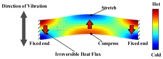
Figure 1.
Sketch map of the regime of thermoelastic damping (TED). As the clamped-clamped microbeam resonator vibrates in a purely flexural mode, one side along the thickness of the beam stretches, which causes the temperature of the region to decrease. The temperature of the compressed side increases, causing a temperature gradient along the thickness of the beam. The irreversible heat flux induced by the temperature gradient causes the dissipation of energy.
Compared with the traditional undamped dynamic system, the introduction of the dissipative source of thermoelastic damping led to a fully coupled thermodynamic system. The governing equations of the motion and heat conduction of the thermoelastically damped systems will be derived in the next part.
2.1. Governing Equation
In the case of a thermoelastically coupled system, the eigenproblem becomes complex and is the main concern here. For problems considering thermoelastic damping, the thermal dilation term is taken into account in the equation of momentum. The equations of motion for the generalized thermodynamic problem can be formulated in matrix form as follows:
where is the displacement vector and is the temperature vector. In this study, we consider that is a positive definite lumped mass matrix and is a non-negative definite symmetric stiffness matrix. The lumped mass matrix is a diagonal positive definite matrix obtained from the traditional consistent mass matrix [36,37]. The lumped mass matrix is widely used in finite element dynamical analyses, and its accuracy has been validated in numerical examples [38,39]. The diagonal elements of the lumped matrix are rational to the corresponding diagonal elements of the original consistent mass matrix. Furthermore, the sums of all elements of the two mass matrices are assumed to be equal such that
where ∑ is a conventional operator for the summation of the elements in the matrix. We will use for the lumped matrix hereafter for simplicity. The matrix of thermal dilation is the coupled term in the equation of motion. Note that even if the lumped mass matrix is singular (e.g., it can be encountered in finite element analysis involving shell elements), the mass matrix can also be formed to be non-singular by introducing the Guyan reduced method [40].
On the other hand, the governing equation of heat conduction takes the following form:
where , and are the matrices of thermal conductivity, heat generation, and heat generation coupled by deformation, respectively. Similar to the mass matrix in the governing equation of motion, the heat generation matrix in the equation of heat conduction is constructed to be a positive definite lumped matrix. A more detailed derivation of the governing equations of the thermodynamically coupled system can be found in [32] and [7].
Notice that both the equations of motion and heat conduction contain the coupled terms. This indicates that they have to be solved simultaneously for the fully coupled system. To overcome the effect of higher-order time derivatives in the system equations of motion and heat conduction, a transformation is applied to the system equations to reduce the order of the thermoelastically coupled system, despite the increased dimensionality of the eigenvalue problem [41]. The traditional direct combination of governing equations is listed below [7]:
where is the identity matrix. Notice that both fixed terms in the equation are asymmetric, which leads to the fact that the direct solution of this equation will suffer a severe computational cost due to the inverse and decomposition processes of the global matrices. To avoid the time-consuming decomposition and inverse step of the solution, the lumped system matrices and are considered in constructing the same term in the transformation to reduce the calculation time. Thus, the combined equation can be constructed in a form similar to the standard dynamic problem and maximally retain the original structure of the governing equations [42]. Combining the governing equations of motion (Equation(1)) and heat conduction (Equation (3)) in the way mentioned before yields
Equation (5) is the eigenvalue problem for a thermoelastically damped microsystem under free vibration. It is clear that the second matrix term in Equation (5) is asymmetric and may not be positive definite, which would significantly increase the computational cost of solving the combined complex eigenvalue problem. However, the first term in Equation (5) is constructed as a diagonal matrix, and the inverse step would cost much less time than in Equation (4).
For the free vibration considered here, to solve the combined equation (Equation (5)), we assume a solution in the form of
where is the ith eigenvalue of the thermoelastically coupled system and and are the amplitudes of the temperature and displacement, respectively.
Then, Equation (5) can be rewritten in the following form:
Note that we construct the combined matrix as a lumped matrix, while is asymmetric. This leads to a complex value for eigenvalue .
2.2. Topology Optimization
The objective of the topology optimization process is to reduce the thermoelastic dissipation of the microbeam resonator. The thermoelastic dissipative ratio can be calculated by dividing the imaginary part of the eigenvalue of the system into its real part [6,43]:
where and denote the imaginary and real part of , respectively.
An iterative bidirectional evolutionary structural optimization (BESO) method for thermoelastic dissipation of a first-order mode shape can be constructed as follows:
where is the design variable (elemental pseudo-density) and is a minimum positive number near 0 to avoid singularity in the finite element analysis process. and are the elemental and global volumes, respectively, is the volume constraint factor, and is the total number of the finite element mesh. The combined governing equation (Equation (9a)) is the main constraint of the optimization problem, along with the standard BESO topology optimization volume constraint in Equation (9b) and design variable constraint in Equation (9c).
According to the definition of thermoelastic dissipation (8) and the complex eigenvalue problem (7), the sensitivity of the objective function with respect to design variable can be obtained through the chain rule as follows [44]:
where the sensitivity of the ith eigenvalue of the system can be obtained through
where is the left eigenvector of the system.
The process of the gradient-based iterative optimization method can be discretized into several steps, as shown in Figure 2. The main task of the iterative optimization process is to obtain the sensitivity numbers of elements through the modal modification analysis process.
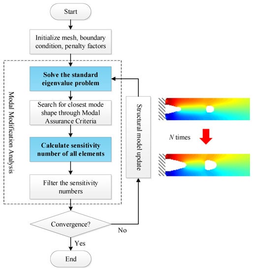
Figure 2.
Flowchart of the topology optimization process.
Marked in blue in Figure 2, the solution of the eigenvalue problem and calculation of global sensitivity numbers are the most time- and computational effort-consuming steps of the modal modification analysis process. As mentioned before, the complex eigenvalue problem for large-scale models is difficult and time-consuming to solve. Due to the change in the material distribution of the structure during the iterative process of topology optimization, the system matrices and eigenvalue problems are altered in each iteration. According to Equations (10) and (11), the sensitivity of the objective function with respect to the design variable is dependent on the mode shape of the system. This leads to the fact that the optimization process requires repeated complex modal analysis of the system in each iteration, which will further prolong the existing time-consuming task.
On the other hand, the observation of the sensitivity equation (Equation (10)) shows that for large-scale models with massive degrees of freedom, solving the sensitivity number of the whole system at one time could be difficult (or even impossible). For this, the sensitivity number of each element has to be solved at the element scale and aggregated to a global matrix. This process can be observed in many examples of research on topology optimization considering static problems [33,34]. However, for thermoelastic coupled systems with complex eigenvalues and eigenvectors, the serial solution method can take a significant amount of time to solve for the element sensitivity numbers. To make matters worse, sensitivity analysis must be performed at each iteration of the optimization process.
The computational and memory effort of the modal modification analysis for the iterative optimization problem of large-scale thermomechanical coupled systems may become unbearable, especially when the problem features a slow convergence requiring tens or even hundreds of iterations. The repeated updating of parametrized designs becomes, therefore, computationally challenging. An efficient modal modification method for repeated analyses of both the eigenproblem and eigensensitivity within gradient-based topology optimization of thermoelastic structures is therefore proposed herein to resolve this computational challenge. As the sensitivity number is dependent on the complex eigenvalue of the system, an efficient modal repeated analysis method is proposed herein to solve the ever-changing eigenvalue problem and mode shape in each iteration of the optimization process. Then, since the sensitivity number of each element is independent of each other, a parallel method is adopted for the process of calculating the sensitivity number of all elements in the thermoelastically coupled structure.
3. Efficient Modal Modification Analysis Method
To efficiently predict the modified modes in each iteration of the topology optimization process, a novel efficient method is presented by combining the Neumann series approximation and the reduced-basis preconditioner technique. The lumped matrices in Equation (2) are used in the matrix decomposition and inverse step to reduce the computational cost of the eigensolution. The Neumann series expansion is usually used to approximately calculate the inverse matrix. The basic character of the Neumann series expansion can be expressed as
where is a identity matrix. The Neumann series expansion converges to the exact value if and only if all the absolute values of the eigenvalues of are less than one; that is, the spectral radius of matrix should be less than the unity. Additionally, the rate of convergence can increase with the decrease in the value of the spectral radius of matrix .
The reduced-basis preconditioner method is one of the most important reduced-order-modeling methods and has been successfully implemented in the solutions of many dynamical systems [45,46]. The reduced-basis preconditioner method seeks an approximation of the high-fidelity solution of the eigenproblem in a reduced space, which is spanned by a set of bases obtained through linear combinations of the solutions of the original eigenproblem.
3.1. Neumann Series Expansion- and Reduced Basis-Based Preconditioner Method
As stated before, the mass and heat generation matrices are lumped matrices to efficiently solve the combined equation. A Neumann series expansion- and reduced basis-based preconditioner method is proposed herein.
Due to the fully coupled characteristic of the system, the coupled terms in governing the equations of motion (Equation (1)) and heat conduction (Equation (3)) have to be solved at the same time. For two-dimensional thermoelastically coupled eigenvalue problems, the degrees of freedom of the system is (including the displacement and temperature ), where is the number of nodes. Thus, the traditional solution of the combined equation (Equation (5)) suffers an increase in the dimensions of . The increase in computational cost could be further magnified by the decomposition and inverse process of the solution. The Krylov subspace-based methods are often used to solve the eigenvalue problems for their simplicity and efficiency in generating orthonormalized bases [47,48]. The standard Krylov method of the standard eigenvalue problem in the form of Equation (7) can be formulated as [49]
However, considering the increase in the dimensions and repeated process in the optimization procedure, solving the eigenproblem directly with the traditional Krylov method could be time- and computational cost-consuming. Thus, we use a Neumann series expansion based technique to construct a lower-order subspace of the system.
As mentioned above, structural modification is encountered frequently in each iteration of the topology’s optimal designs to enhance the performance of structural or mechanical systems by altering their substructures. Suppose a change in the design parameters resulting in modified system matrices, which can be expressed as
Here, and are the modified matrices. and denote the change in the system matrices.
The modified eigenproblem can then become
A preconditioner is used here to turn this eigenproblem into a standard Neumann series expansion form. The preconditioners have been widely used in the solution of linear partial differential equations within finite element eigenvalue problems [50,51], which occur frequently in thermal and dynamical systems. There are many types of preconditioners, including the diagonal preconditioners, the reduced-basis preconditioners, and the differential preconditioners, which can be interpreted as a differential operator [45,52]. The preconditioners are frequently (or even necessarily) used in the subspace solutions of partial differential equations [53]. Based on different types of preconditioners, preconditioned iterative methods were proposed to solve large-scale eigenproblems with a slow convergence [47]. Among all the types of preconditioners, the diagonal preconditioner is famous for its simplicity and fast convergence. Thus, a diagonal preconditioner is chosen herein and pre-multiplied to the modified eigenproblem in Equation (15) [54]. Note that for a specific ith mode shape, the system eigenvalue is scalar, while the system matrix has been constructed as a diagonal matrix. Thus, the preconditioner adds little to the computational effort of the inverse step in constructing the basis. With the help of the preconditioner and Equation (14), one obtains
where
Next, we will use the Neumann series expansion to approximate the modified mode shapes. The process of obtaining an r-order Neumann basis procedure is shown in Algorithm 1. By using the Neumann series expansion, one obtains
On the condition that the mode shapes do not change significantly, it may be convenient to approximate the eigenvectors with known mode shapes:
where
As stated before, the calculation of the basis vectors requires the inverse of the matrix , whose operation count is trivial due to the fact that it is constructed as a diagonal matrix. Thus, we define the r-order Neumann series expansion-based Krylov subspace as [48]
It is clear that the Neumann series expansion-based subspace is constructed as a linear combination of the traditional subspace . Note that is a diagonal matrix, and the inverse process could be easy since the basis vectors can be efficiently calculated by only sparse matrix multiplications using a simple iterative procedure. However, the coefficients of each basis vector are still unknown and, therefore, need to be determined based on a preconditioner technique. Next, we introduce the reduced-basis-based preconditioner technique to solve these coefficients.
| Algorithm 1: Neumann basis procedure |
 |
With the proposed r-order Neumann subspace basis vectors, the modified mode shape vector can be rewritten as
where denotes the matrix of the explicit Neumann series expansion-based Krylov basis of and
Since the approximate eigenvectors should satisfy the eigenproblem in Equation (15), the unknown coefficients can be determined by substituting the approximate eigenvectors back into Equation (15). However, note that the solution of the unknown coefficients of may still be time-consuming, since the dimensions of Equation (15) are still .
To reduce the dimension of the system and maintain the robustness of the system’s eigenvalue problem, a reduced-basis preconditioner is used here. As stated before, the reduced-basis preconditioner technique requires the linear combination of the original high-fidelity subspace, which was obtained through Equations (20) and (22). Thus, the transpose of the basis matrix , a rectangular reduced-basis preconditioner is chosen here and pre-multiplied to the corresponding high-fidelity terms in Equation (15) [55]:
As is a reduced-basis preconditioner and may not be a Hermitian matrix, the robustness of the rectangular basis matrix has to be improved by using a Gram–Schmidt orthonormalization (GSO) procedure. The GSO procedure is shown in Algorithm 2, where denotes the modulus of the vector and denotes the inner product the two vector elements; that is, the rectangular basis matrix should be normalized to such that each column of it becomes uncoupled and becomes .
| Algorithm 2: GSO procedure |
 |
Finally, the solution of the eigenproblem in Equation (15) can be replaced by solving a smaller one, defined as
The reduced system matrices are dense matrices, but they are symmetric and much smaller in size than the original system matrices. The approximate modified eigenvalue can be chosen by finding the absolute smallest eigenvalue of the reduced eigenproblem in Equation (25). This means that only the first-order mode of the reduced eigenproblem needs to be solved. This method allows the size of the problem to be decreased remarkably (the reduced size is ) so that the computational effort can be reduced remarkably. Once the vector is calculated, the modified eigenvectors can be obtained through Equation (22).
3.1.1. Procedure of the Proposed Preconditioner Method
The procedure of the proposed method shown in Figure 3 can be summarized as follows.
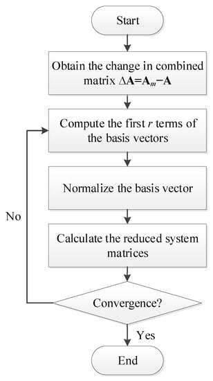
Figure 3.
Flowchart of the modal repeated analysis method.
Step 1: Obtain the change in the combined matrix by ;
Step 2: Compute the first r terms of the basis vectors by using Equation (20). Since the lumped matrices and are diagonal, the inverse of the combined matrix is trivial. Thus, the basis vector can be efficiently calculated by only sparse matrix multiplications. The algorithm for obtaining the basis vectors is given in Algorithm 1;
Step 3: Normalize the basis vector using the Gram–Schmidt orthonormalization procedure in Algorithm 2. Note that the basis vectors will become linearly dependent if a large value of the number r is chosen. With the Gram–Schmidt orthonormalization algorithm, the proposed method is robust;
Step 4: Calculate the reduced system matrices by Equation (24) and solve the reduced eigenproblem in Equation (25) for the first-order mode. The eigenvalue of the first-order mode is the modified eigenvalue ;
Step 5: Validate the convergence of the Neumann series expansion with the spectral radius of the expanded term in Equation (16).
3.1.2. Convergence Condition and Relative Computational Effort of the Neumann Series Expansion
As stated before, the convergence of a Neumann series expansion depends on the eigenvalues of the non-identity term. For the convergent Neumann series expansion in Equation (18), one obtains the necessary and sufficient condition
Here, denotes the spectral radius of the matrix . This means that all the eigenvalues of the matrix have absolute values less than one. The maximum eigenvalues of the matrix can be found by solving the minimum eigenvalues of the following eigenproblem:
Once the minimum eigenvalue is solved, the convergence condition can be given by
By considering the relationship in Equation (17), we obtain
which can be approximately determined using the known undamped (real) frequencies:
For structures modeled by the lumped mass matrix and heat generation matrix , the system matrix is a diagonal matrix, and the operation count for the matrix decomposition of is trivial. The process of forward and backward substitutions for these basis vectors is for real matrices and for complex matrices, where b is the semi-bandwidth of the combined matrix and L is the number of the modes of interest. Since the number of the basis vectors and the number of the calculated modes , the other operation count is trivial. Since the half-bandwidth b is roughly proportional to [56], the operation count is simplified as in the case of real modal analysis and in the case of complex modal analysis. Therefore, the proposed repeated analysis method shows a clear advantage in the eigenvalue analysis step and thus results in an improvement over the full analysis in engineering and optimization applications.
It is worth noting that solving the complex eigenvalue problem is not an end in itself, as the final goal of the modal analysis of the optimization process is to obtain the sensitivity number with respect to the design variable. Thus, the repeated analysis method is implemented in an optimization process along with the parallel sensitivity analysis technique.
3.2. Parallel Sensitivity Analysis Technique
As shown in Figure 2, calculating the sensitivity numbers of all elements is the other of the two time-consuming steps of the iterative optimization process. To reduce the computational effort of the sensitivity analysis process, a parallel computational technique is adopted for calculation of the global sensitivity numbers.
The parallel technique has been widely used recently for better computer performance. There are dense parallel techniques that can be inferred as several patterns: the master-slave pattern [57], the divide-and-conquer pattern [58], speculative multithreading [59], etc. The master-slave pattern is the most representative distributed pattern and contains two parts: the master node and slave nodes. The master takes full responsibility for the main task, and the slaves deal with independent subtasks. The divide-and-conquer pattern aims to divide the main task into several subtasks, where some of the subtasks are dependent on each other and are aggregated before others to obtain an integrated solution of the subtasks. The speculative multithreading parallelizes the sequential codes aggresively, while the hardware guarantees the success of the execution [60].
The master-slave pattern, among all alternatives, is widely used for its ease of implementation and relatively better convergence capabilities [29]. Thus, we choose the master-slave parallel pattern for the parallel analysis of the matrix of global sensitivity numbers.
The master-slave pattern herein is organized into three layers, as shown in Figure 4. The task layer contains the main task of the entire parallel program (i.e., to obtain the global matrix of sensitivity numbers of the eigenvalue with respect to the elemental pseudo-densities of the thermodynamically coupled system):
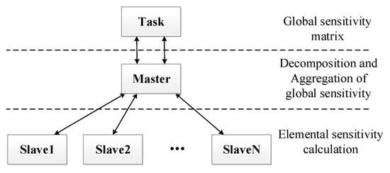
Figure 4.
Sketch map of the parallel method of the master-slave pattern.
The master layer takes full responsibility for the main task. It constructs and manipulates the global sensitivity matrix according to the demand of the main task. The slave layer handles the subtasks assigned by the master to calculate the sensitivity number of each element.
The flow of the master-slave parallel algorithm is shown in Algorithm 3.
The master node handles task decomposition and collects feedback for each subtask. Recalling the definition of the eigenvalue part of the system in Equation (11), the sensitivity numbers of the elements are independent of each other. This in turn shows that the sensitivity of the ith eigenvalue to the eth element’s pseudo-density can be solved at the element scale with the reduced system matrix. The ith system’s mode shape of the modified structure can be obtained with Equation (22).
| Algorithm 3: Master-slave parallel procedure |
 |
For the eth element, as messages of other elements are not necessary for computing the elemental sensitivity number, the system matrix can be replaced by , where is a conventional operator retaining the message of the eth element and neglecting others. Other system matrices can be replaced in a similar way for the elemental calculation.
Thus, the elemental sensitivity number of the eth element of the ith mode shape can be solved by
The slave nodes in the slave layer are solely responsible for their assigned subtasks, which is to solve the elemental sensitivity matrix in Equation (10) with the help of the elemental sensitivity number of the eigenvalue with respect to the design variable in Equation (32). The input and output of the eth subtask are the extracted system matrices and eth elemental sensitivity numbers, respectively.
The master-slave pattern can be distributed among different computers and use the remote procedure call to communicate with each other or be distributed in one computer among different cores of the CPU. As the time delay between different computers is significantly larger than that between the cores of the CPU of the same computer, in some cases, the time cost of a data transfer may strongly influence the total computational time of the parallel process. To balance the time cost between the computational time within a slave node and the transferring time between the master and slaves, the master-slave parallel technique is implemented in one computer here. The master-slave pattern developed here may also be useful for the repeated eigenvalue sensitivity analysis arising in different subjects [44,61,62,63,64], and further research in this direction is worth pursuing.
4. Results and Discussion
In this study, the efficient repeated analysis- and parallel-based modal modification analysis method proposed was compared to the traditional method with two examples of thermodynamically damped systems. The efficient reduced-basis preconditioner method and parallel technique of calculation of the sensitivity number developed herein were compared to the traditional subspace method and linear computation of the sensitivity number in an iterative topology optimization process for complex eigenfrequency and sensitivity analysis [32].
The proposed repeated analysis method was implemented in an iterative topology optimization process to validate its accuracy and computational cost, and the examples were constructed in Matlab. As stated before, the convergence of the Neumann series expansion was dependent on the spectral radius of the term in parentheses in Equation (12). However, in was altered each time as the material distribution changed in the topology optimization process. Thus, a posterior validation of the convergence of the Neumann series expansion was conducted in each iteration of the optimization process.
The same material parameters and evolutionary optimization parameters were implemented in the topology optimization process for the traditional linear method and the proposed repeated analysis- and parallel-based method. The material properties were a Young’s modulus of , density of , Poisson’s ratio of 0.22, thermal expansion coefficient of , specific heat per unit mass of , and thermal conductivity of with no penalty applied to these parameters. The evolutionary optimization parameters were set to a volume limitation of 0.8, evolutionary rate for each iteration of 0.01, and mesh-independent filter radius of 4. A normalization process was adopted for the objective function for better comparison.
A clamped-clamped microbeam resonator of μm was chosen as a numeric example for optimizing the quality factor of the first-order mode shape, where both the proposed method and traditional method were implemented in the finite element analysis process for a complex eigenvalue solution. The whole design region was discretized into a finite element mesh with a total of 49,323 degrees of freedom (DOFs), including the displacement and temperature.
The optimization results with the traditional subspace method and the proposed method () for finite element analysis are shown in Figure 5.
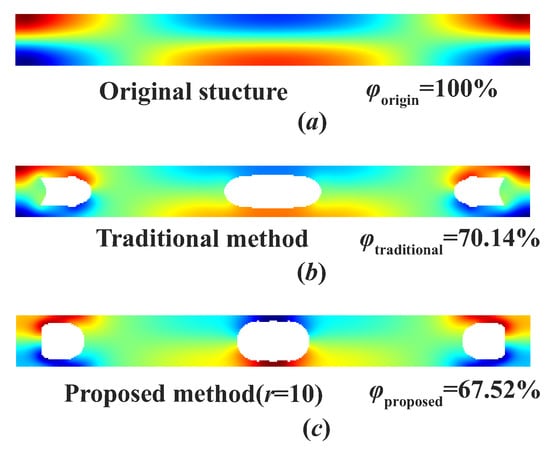
Figure 5.
Topology optimization results for a clamped-clamped microbeam resonator. (a) The original structure. (b) The optimization result where the traditional subspace method is implemented in the finite element analysis step. (c) The optimization result where the proposed method is implemented in the finite element analysis step.
It can be observed in the optimized structure for the traditional method (Figure 5b) and the proposed method (Figure 5c) that the positions of the main voids were nearly the same, which indicates that the main optimizing directions of the optimization methods containing two different eigenvalue solution methods were the same. The difference at the border of the voids may be explained by the truncation error, which may slightly affect the local optimizing direction of the topology optimization method. On the other hand, the error of the normalized thermoelastic dissipation rate was also acceptable, and the optimized structure for the proposed method even had a better dissipative rate than the optimized structure conducted by the traditional subspace method. The average computation time of the step of the solution of the complex eigenvalue problem in each iteration for the traditional subspace method was 4.3108 s, while the computation time of the same step for the proposed method was 1.5779 s, as shown in Table 1. The average computation time of the linear calculation of the global matrix of the sensitivity number was 6.1492 s, while the computation time of the same step in a parallel method was 0.9175 s. The modal assurance criteria and filter of the sensitivity numbers were simple vector multiplications and cost little computation effort. Thus, the proposed method saved approximately 76.14% of the computation time compared with the traditional linear method for sensitivity analysis of the topology optimization process of a clamped-clamped microbeam resonator.

Table 1.
The comparison of the average computational times of each iteration of topology optimization of the clamped-clamped microbeam resonator with the traditional linear method and the proposed method.
Similarly, a clamped-free microbeam resonator of 30 × 6 μm was chosen as a numeric example for comparison. The whole design region was discretized into a 300 × 60 finite element mesh with a total of 55,083 DOFs, including the displacement and temperature.
It can be observed in the optimized structure for the traditional method (Figure 6b) and the proposed method (Figure 6c) that the void regions near the clamped side and in the middle were quite alike, with some difference at the border.
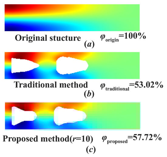
Figure 6.
Topology optimization results for a clamped-free microbeam resonator. (a) The original structure. (b) The optimization result where the traditional subspace method is implemented in the finite element analysis step. (c) The optimization result where the proposed method is implemented in the finite element analysis step.
This may be because the truncation error may affect the local optimizing direction of the topology optimization method. Once again, the error of the normalized thermoelastic dissipation rate was acceptable, and the computational efficiency was improved significantly for the proposed method, as shown in Table 2.
Table 2.
The comparison of the average computational times of each iteration of topology optimization of the clamped-free microbeam resonator with the traditional linear method and the proposed method.
Thus, the proposed method saved significant computation time in comparison with the traditional linear method for the sensitivity analysis of the thermodynamically coupled system, with little loss of accuracy of the optimization result.
5. Concluding Remarks
Thermoelastically coupled microresonators are widely applied in micro-electronic mechanical systems. The dense research on the main characteristics (resonant frequency and dissipative rate) of microresonators and the maturing of manufacturing technology leads to the demand for design methods for microstructures. The computation cost of repeated sensitivity analysis of a large-scale, fully thermoelastically coupled system in optimization iterations is extremely high. There is still a lack of an efficient modal modification method in the gradient-based topology optimization of a large-scale, fully coupled thermoelastic system, although there are some works for standard eigenproblems and their sensitivities. To this end, a modal modification analysis method was proposed herein to efficiently update the eigenvalues and their sensitivities in gradient-based topology optimization for thermoelastic systems, which is essential when dealing with their complex eigenproblem and global sensitivity analysis for a huge number of design parameters. The feasibility of the modal modification analysis method for large-scale, fully coupled thermoelastic structures is demonstrated in the gradient-based topology optimization problem. The modal modification analysis method is useful for the repeated eigenvalue analysis of thermoelastic structures arising in different subjects, including conceptual design problems, structural optimization, damage analysis, probabilistic analysis, structural control, and smart or adaptive structures.
The two most time-consuming and computationally expensive steps in sensitivity analysis were analyzed, and a targeted efficiency improvement method was proposed. The modal modification analysis technique gives efficient procedures to obtain the eigensolution due to the changes in the design parameters of the system without having to repeat the equilibrium equation several times. A novel, efficient Neumann series expansion- and reduced-basis-based preconditioner method was presented for the modal analysis of the structures modeled by the lumped mass and heat generation matrices. The characteristic of the lumped combined matrix (diagonal) led to a trivial operation count, while the basis vector could be efficiently calculated by only sparse matrix multiplications using a simple iterative procedure. The sufficient condition for the Neumann series approximation was derived, and the computational complexity of the proposed method was also discussed. On the other hand, the master-slave pattern parallel technique was adopted for the solution of the global sensitivity numbers. The sensitivity numbers were solved at the element scale within the slave nodes and aggregated to the global sensitivity matrix by the master node.
Finally, two case studies were used to illustrate the effectiveness of the proposed method. The proposed modal modification analysis method was implemented in an iterative topology optimization process of reducing thermoelastic dissipation. A comparison between the proposed method and the traditional method was conducted in terms of the optimization results and computation times. It was shown by the two case studies that the proposed method showed a clear advantage in the computational cost with little loss of accuracy. The solution steps are straightforward, and the proposed method can be easily implemented in general purpose finite element software.
The proposed modal modification analysis method may be useful for the repeated eigenvalue analysis of thermoelastic structures arising in different subjects, including conceptual design problems, structural optimization, damage analysis, probabilistic analysis, structural control, and smart or adaptive structures. Furthermore, there are other computationally challenging problems for different multiphysical systems, such as electro-mechanical coupled systems and piezo-elastic systems, which may result in tremendous computational times of the optimization frameworks for these systems. Thus, the research conducted here can be helpful for accelerating recent developments in the analysis and design of thermoelastic structures as well as microresonators for engineering applications, and further research in this direction is worth pursuing.
Author Contributions
Y.F.: methodology, software, investigation, formal analysis, and writing—original draft; L.L.: conceptualization, methodology, writing—review and editing, supervision, and funding acquisition; Y.H.: methodology, writing—review and editing, resource, and project administration. All authors have read and agreed to the published version of this manuscript.
Funding
This work was supported by the National Key Research and Development Program of China (grant no. 2021YFB1714600), the National Natural Science Foundation of China (grant no. 52175095), and the Young Top-Notch Talent Cultivation Program of Hubei Province of China.
Institutional Review Board Statement
Not applicable.
Informed Consent Statement
Not applicable.
Data Availability Statement
Not applicable.
Conflicts of Interest
The authors declare no conflict of interest.
References
- Shi, J.; Liu, S.; Zhang, L.; Yang, B.; Shu, L.; Yang, Y.; Ren, M.; Wang, Y.; Chen, J.; Chen, W. Smart textile-integrated microelectronic systems for wearable applications. Adv. Mater. 2020, 32, 1901958. [Google Scholar] [CrossRef]
- Kim, B.; Candler, R.N.; Hopcroft, M.A.; Agarwal, M.; Park, W.T.; Kenny, T.W. Frequency stability of wafer-scale film encapsulated silicon based MEMS resonators. Sens. Actuators Phys. 2007, 136, 125–131. [Google Scholar] [CrossRef]
- Sandberg, R.; Mølhave, K.; Boisen, A.; Svendsen, W. Effect of gold coating on the Q-factor of a resonant cantilever. J. Micromech. Microeng. 2005, 15, 2249–2253. [Google Scholar] [CrossRef]
- Hao, Q.; Chen, G.; Jeng, M.S. Frequency-dependent Monte Carlo simulations of phonon transport in two-dimensional porous silicon with aligned pores. J. Appl. Phys. 2009, 106, 114321. [Google Scholar] [CrossRef]
- Biot, M.A. Thermoelasticity and Irreversible Thermodynamics. J. Appl. Phys. 1956, 27, 240–253. [Google Scholar] [CrossRef]
- Lifshitz, R.; Roukes, M.L. Thermoelastic damping in micro-and nanomechanical systems. Phys. Rev. B 2000, 61, 5600. [Google Scholar] [CrossRef]
- Guo, X.; Yi, Y.B.; Pourkamali, S. A finite element analysis of thermoelastic damping in vented MEMS beam resonators. Int. J. Mech. Sci. 2013, 74, 73–82. [Google Scholar] [CrossRef]
- Sherief, H.H.; Hussein, E.M. Fundamental solution of thermoelasticity with two relaxation times for an infinite spherically symmetric space. Z. Angew. Math. Phys. 2017, 68, 1–14. [Google Scholar] [CrossRef]
- Sherief, H.H.; Hussein, E.M. Contour integration solution for a thermoelastic problem of a spherical cavity. Appl. Math. Comput. 2018, 320, 557–571. [Google Scholar] [CrossRef]
- Hussein, E.M. Mathematical model for thermoelastic Porous spherical region problems. Comput. Therm. Sci. Int. J. 2020, 12. [Google Scholar] [CrossRef]
- Hussein, E.M. Mathematical model for thermo-poroelastic plate saturated with fluid. Spec. Top. Rev. Porous Media Int. J. 2020, 11. [Google Scholar] [CrossRef]
- Fu, H.; Nan, K.; Bai, W.; Huang, W.; Bai, K.; Lu, L.; Zhou, C.; Liu, Y.; Liu, F.; Wang, J. Morphable 3D mesostructures and microelectronic devices by multistable buckling mechanics. Nat. Mater. 2018, 17, 268–276. [Google Scholar] [CrossRef] [PubMed]
- Meng, L.; Zhang, W.; Quan, D.; Shi, G.; Tang, L.; Hou, Y.; Breitkopf, P.; Zhu, J.; Gao, T. From Topology Optimization Design to Additive Manufacturing: Today’s Success and Tomorrow’s Roadmap. Arch. Comput. Methods Eng. 2019, 27, 805–830. [Google Scholar] [CrossRef]
- Fu, Y.; Li, L.; Duan, K.; Hu, Y. A thermodynamic design methodology for achieving ultra-high frequency–quality product of microresonators. Thin-Walled Struct. 2021, 166, 108104. [Google Scholar] [CrossRef]
- Lohan, D.J.; Dede, E.M.; Allison, J.T. Topology optimization for heat conduction using generative design algorithms. Struct. Multidiscip. Optim. 2016, 55, 1063–1077. [Google Scholar] [CrossRef]
- Deng, S.; Suresh, K. Stress constrained thermo-elastic topology optimization with varying temperature fields via augmented topological sensitivity based level-set. Struct. Multidiscip. Optim. 2017, 56, 1413–1427. [Google Scholar] [CrossRef]
- Zhu, X.; Zhao, C.; Wang, X.; Zhou, Y.; Hu, P.; Ma, Z.D. Temperature-constrained topology optimization of thermo-mechanical coupled problems. Eng. Optim. 2019, 51, 1687–1709. [Google Scholar] [CrossRef]
- Gao, T.; Zhang, W. Topology optimization involving thermo-elastic stress loads. Struct. Multidiscip. Optim. 2010, 42, 725–738. [Google Scholar] [CrossRef]
- Homayouni-Amlashi, A.; Schlinquer, T.; Mohand-Ousaid, A.; Rakotondrabe, M. 2D topology optimization MATLAB codes for piezoelectric actuators and energy harvesters. Struct. Multidiscip. Optim. 2020, 63, 983–1014. [Google Scholar] [CrossRef]
- Candler, R.N.; Duwel, A.; Varghese, M.; Chandorkar, S.A.; Hopcroft, M.A.; Park, W.T.; Kim, B.; Yama, G.; Partridge, A.; Lutz, M. Impact of geometry on thermoelastic dissipation in micromechanical resonant beams. J. Microelectromech. Syst. 2006, 15, 927–934. [Google Scholar] [CrossRef]
- Choi, K.K.; Kim, N.H. Structural Sensitivity Analysis and Optimization 1: Linear Systems; Springer Science and Business Media: New York, NY, USA, 2004. [Google Scholar]
- Chen, J.C.; Wada, B. Matrix perturbation for structural dynamic analysis. AIAA J. 1977, 15, 1095–1100. [Google Scholar] [CrossRef]
- Dedieu, J.P.; Tisseur, F. Perturbation theory for homogeneous polynomial eigenvalue problems. Linear Algebra Its Appl. 2003, 358, 71–94. [Google Scholar] [CrossRef]
- Li, L.; Hu, Y.J.; Wang, X.L. Modal modification of damped asymmetric systems without using the left eigenvectors. Proc. Appl. Mech. Mater. 2014, 490, 331–335. [Google Scholar] [CrossRef]
- Noor, A.K. Recent advances and applications of reduction methods. Appl. Mech. Rev. 1994, 125–146. [Google Scholar] [CrossRef]
- Kirsch, U. Reanalysis and sensitivity reanalysis by combined approximations. Struct. Multidiscip. Optim. 2010, 40, 1–15. [Google Scholar] [CrossRef]
- Sadeeq, M.M.; Abdulkareem, N.M.; Zeebaree, S.R.; Ahmed, D.M.; Sami, A.S.; Zebari, R.R. IoT and Cloud computing issues, challenges and opportunities: A review. Qubahan Acad. J. 2021, 1, 1–7. [Google Scholar] [CrossRef]
- Shao, W.; Yao, L.; Ge, Z.; Song, Z. Parallel computing and SGD-based DPMM for soft sensor development with large-scale semisupervised data. IEEE Trans. Ind. Electron. 2018, 66, 6362–6373. [Google Scholar] [CrossRef]
- Turgut, M.S.; Turgut, O.E.; Afan, H.A.; El-Shafie, A. A novel Master–Slave optimization algorithm for generating an optimal release policy in case of reservoir operation. J. Hydrol. 2019, 577, 123959. [Google Scholar] [CrossRef]
- Šimkus, A.; Turskienė, S. Parallel computing for the finite element method in MATLAB. Comput. Sci. Tech. 2013, 1, 214–221. [Google Scholar] [CrossRef][Green Version]
- Zhang, B.; Xu, S.; Zhang, F.; Bi, Y.; Huang, L. Accelerating matlab code using gpu: A review of tools and strategies. In Proceedings of the 2011 2nd International Conference on Artificial Intelligence, Management Science and Electronic Commerce (AIMSEC), Zhengzhou, China, 8–10 August 2011; pp. 1875–1878. [Google Scholar] [CrossRef]
- Fu, Y.; Li, L.; Hu, Y. Enlarging quality factor in microbeam resonators by topology optimization. J. Therm. Stress. 2019, 42, 341–360. [Google Scholar] [CrossRef]
- Sigmund, O. A 99 line topology optimization code written in Matlab. Struct. Multidiscip. Optim. 2001, 21, 120–127. [Google Scholar] [CrossRef]
- Huang, X.; Xie, Y.M. Evolutionary topology optimization of continuum structures with an additional displacement constraint. Struct. Multidiscip. Optim. 2009, 40, 409–416. [Google Scholar] [CrossRef]
- Jinling, Y.; Ono, T.; Esashi, M. Energy dissipation in submicrometer thick single-crystal silicon cantilevers. J. Microelectromech. Syst. 2002, 11, 775–783. [Google Scholar] [CrossRef]
- Fried, I.; Malkus, D.S. Finite element mass matrix lumping by numerical integration with no convergence rate loss. Int. J. Solids Struct. 1975, 11, 461–466. [Google Scholar] [CrossRef]
- Kim, K.O. A review of mass matrices for eigenproblems. Comput. Struct. 1993, 46, 1041–1048. [Google Scholar] [CrossRef]
- Jensen, M.S. High convergence order finite elements with lumped mass matrix. Int. J. Numer. Methods Eng. 1996, 39, 1879–1888. [Google Scholar] [CrossRef]
- Wu, S.R. Lumped mass matrix in explicit finite element method for transient dynamics of elasticity. Comput. Methods Appl. Mech. Eng. 2006, 195, 5983–5994. [Google Scholar] [CrossRef]
- Guyan, R.J. Reduction of stiffness and mass matrices. AIAA J. 1965, 3, 380. [Google Scholar] [CrossRef]
- Reddy, J.N.; Gartling, D.K. The Finite Element Method in Heat Transfer and Fluid Dynamics; CRC Series in Computational Mechanics and Applied Analysis; CRC Press: Boca Raton, FL, USA, 2010. [Google Scholar]
- Thomson, W. Theory of Vibration with Applications; CRC Press: Boca Raton, FL, USA, 1996. [Google Scholar]
- Li, L.; Hu, Y.; Deng, W.; Lü, L.; Ding, Z. Dynamics of structural systems with various frequency-dependent damping models. Front. Mech. Eng. 2015, 10, 48–63. [Google Scholar] [CrossRef]
- Li, L.; Hu, Y.; Wang, X. Design sensitivity analysis of dynamic response of nonviscously damped systems. Mech. Syst. Signal Process. 2013, 41, 613–638. [Google Scholar] [CrossRef]
- Ito, K.; Ravindran, S.S. A reduced-order method for simulation and control of fluid flows. J. Comput. Phys. 1998, 143, 403–425. [Google Scholar] [CrossRef]
- Sen, S.; Veroy, K.; Huynh, D.B.P.; Deparis, S.; Nguyen, N.C.; Patera, A.T. “Natural norm” a posteriori error estimators for reduced basis approximations. J. Comput. Phys. 2006, 217, 37–62. [Google Scholar] [CrossRef]
- Saad, Y. Analysis of augmented Krylov subspace methods. SIAM J. Matrix Anal. Appl. 1997, 18, 435–449. [Google Scholar] [CrossRef]
- Bai, Z.; Su, Y. SOAR: A second-order Arnoldi method for the solution of the quadratic eigenvalue problem. SIAM J. Matrix Anal. Appl. 2005, 26, 640–659. [Google Scholar] [CrossRef]
- Bai, Z.; Demmel, J.; Dongarra, J.; Ruhe, A.; van der Vorst, H. Templates for the Solution of Algebraic Eigenvalue Problems: A Practical Guide; SIAM: Philadelphia, PA, USA, 2000. [Google Scholar]
- Kearfott, R.B.; Hu, C.; Novoa, M., III. A review of preconditioners for the interval Gauss-Seidel method. Interval Comput. 1991, 1, 59–85. [Google Scholar]
- Turkel, E. Preconditioning techniques in computational fluid dynamics. Annu. Rev. Fluid Mech. 1999, 31, 385–416. [Google Scholar] [CrossRef]
- Mardal, K.; Winther, R. Preconditioning discretizations of systems of partial differential equations. Numer. Linear Algebra Appl. 2011, 18, 1–40. [Google Scholar] [CrossRef]
- Pearson, J.W.; Pestana, J. Preconditioners for Krylov subspace methods: An overview. GAMM-Mitteilungen 2020, 43, e202000015. [Google Scholar] [CrossRef]
- Cai, X.C.; Sarkis, M. A restricted additive Schwarz preconditioner for general sparse linear systems. SIAM J. Sci. Comput. 1999, 21, 792–797. [Google Scholar] [CrossRef]
- Santo, N.D.; Deparis, S.; Manzoni, A.; Quarteroni, A. Multi space reduced basis preconditioners for large-scale parametrized PDEs. SIAM J. Sci. Comput. 2018, 40, A954–A983. [Google Scholar] [CrossRef]
- Bathe, K.J. Finite Element Procedures; PRENTICE HALL: Upper Saddle River, NJ, USA, 2006. [Google Scholar]
- Li, Y.; Zhang, Z. Parallel computing: Review and perspective. In Proceedings of the 2018 5th International Conference on Information Science and Control Engineering (ICISCE), Zhengzhou, China, 20–22 July 2018; pp. 365–369. [Google Scholar] [CrossRef]
- Mei, Y.; Omidvar, M.N.; Li, X.; Yao, X. A competitive divide-and-conquer algorithm for unconstrained large-scale black-box optimization. ACM Trans. Math. Softw. (TOMS) 2016, 42, 1–24. [Google Scholar] [CrossRef]
- Estebanez, A.; Llanos, D.R.; Gonzalez-Escribano, A. A survey on thread-level speculation techniques. ACM Comput. Surv. (CSUR) 2016, 49, 1–39. [Google Scholar] [CrossRef]
- Bader, D. Analyzing massive social networks using multicore and multithreaded architectures. In Facing the Multicore-Challenge; Springer: Berlin/Heidelberg, Germany, 2010; p. 1. [Google Scholar]
- Li, L.; Hu, Y.; Wang, X. A parallel way for computing eigenvector sensitivity of asymmetric damped systems with distinct and repeated eigenvalues. Mech. Syst. Signal Process. 2012, 30, 61–77. [Google Scholar] [CrossRef]
- Lin, R.; Ng, T. Repeated eigenvalues and their derivatives of structural vibration systems with general nonproportional viscous damping. Mech. Syst. Signal Process. 2021, 159, 107750. [Google Scholar] [CrossRef]
- Li, L.; Hu, Y.; Wang, X. Design sensitivity and Hessian matrix of generalized eigenproblems. Mech. Syst. Signal Process. 2014, 43, 272–294. [Google Scholar] [CrossRef]
- Lin, R.; Mottershead, J.; Ng, T. A state-of-the-art review on theory and engineering applications of eigenvalue and eigenvector derivatives. Mech. Syst. Signal Process. 2020, 138, 106536. [Google Scholar] [CrossRef]
Publisher’s Note: MDPI stays neutral with regard to jurisdictional claims in published maps and institutional affiliations. |
© 2022 by the authors. Licensee MDPI, Basel, Switzerland. This article is an open access article distributed under the terms and conditions of the Creative Commons Attribution (CC BY) license (https://creativecommons.org/licenses/by/4.0/).