

Chaos Particle Swarm Optimization Enhancement Algorithm for UAV Safe Path Planning

Abstract
:1. Introduction
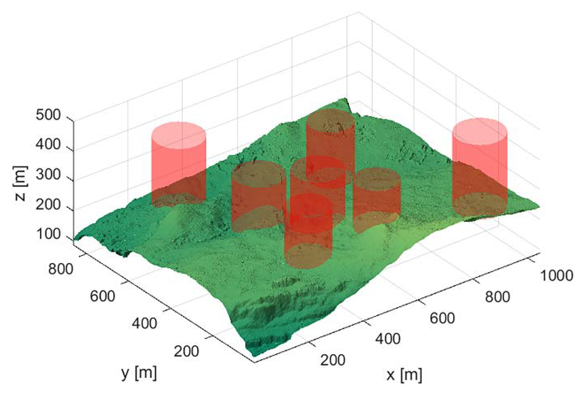
2. Threat Environment Model
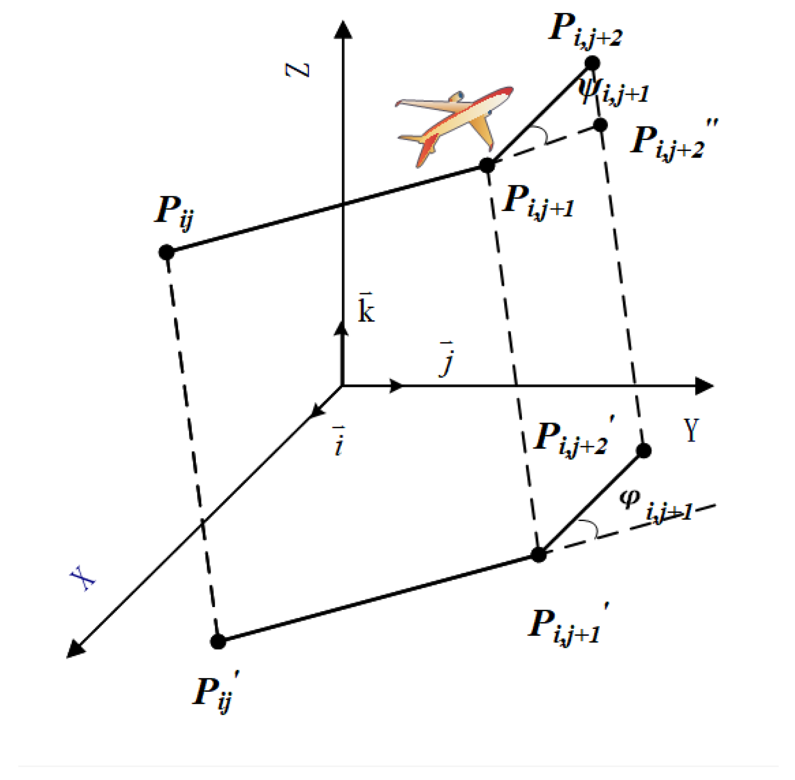
2.1. Optimal Path
2.2. Terrain and UAV Performance Constraints
2.3. Total Cost Function
3. PSO Algorithm
4. Proposed PSO Variant
4.1. VAINDIWPSO Algorithm
4.1.1. Improvements Nonlinear Dynamic Inertial Weights
4.1.2. Update Velocity
4.2. IC-VAINDIWPSO Algorithm
4.2.1. Adaptive Adjustment of Velocity
4.2.2. Chaos Initialization
4.2.3. Logistic Chaos Map
4.2.4. The Specific Steps of the IC-VAINDIWPSO Algorithm
- (a)
- Modeling the threat environment for drone flight;
- (b)
- Initializing the particle swarm with improved chaos theory;
- (c)
- Evaluating particles: according to the constraints in the threat environment, the fitness value of the particles is evaluated;
- (d)
- Updating particles: the particle positions and velocities are updated according to (11) and (19)–(21);
- (e)
- Calculating the rate of change of fitness (FCR) according to (25). If , and FCR is less than the set threshold, the local position of the particle changes slightly, and it falls into the local optimum. Go to (f), otherwise, go to (g);
- (f)
- According to the logistic chaotic map (23), the mutation operation is performed on the global best position;
- (g)
- Stop condition; by iterating continuously, adjust their velocity and position to keep them inside the feasible range until the algorithm reaches the maximum number of iterations and obtains the optimal solution; otherwise, return to (c).
| Algorithm 1 IC-VAINDIWPSO algorithm |
| /* Initialization: */ 1 Obtain search map and initial path planning information; 2 Set swarm parameters, swarm_size; 3 for each particle i in swarm do 4 Create a random path; 5 Assign to particle’s position; 6 Compute fitness of the particle; 7 Set local_best of the particle to its fitness; 8 end 9 Chaos initialization 10 Set global_best to the best-fit particle; /* Evolutions: */ 11 for k ← 1 to max_generation do 12 for each particle i in swarm do 13 Compute velocity; /* Equation (21)*/ 14 if Particles become stuck in local optima 15 Compute velocity; /* Equation (20)*/ 16 end 17 Compute new position; /* Equation (11) */ 18 Update fitness; /* Equation (9) */ 19 if k is less than 2/3 * max_generation 20 Compute FCR /* Equation (25) */ 21 if FCR is less than the set threshold 22 Compute new position; /* Equation (23) */ 23 end 24 end 25 Update local_best; 26 end 27 Update global_best; 28 Update inertia weights /* Equation (19) */ 29 Save best_position associated with global_best; /* the best path */ 30 end |
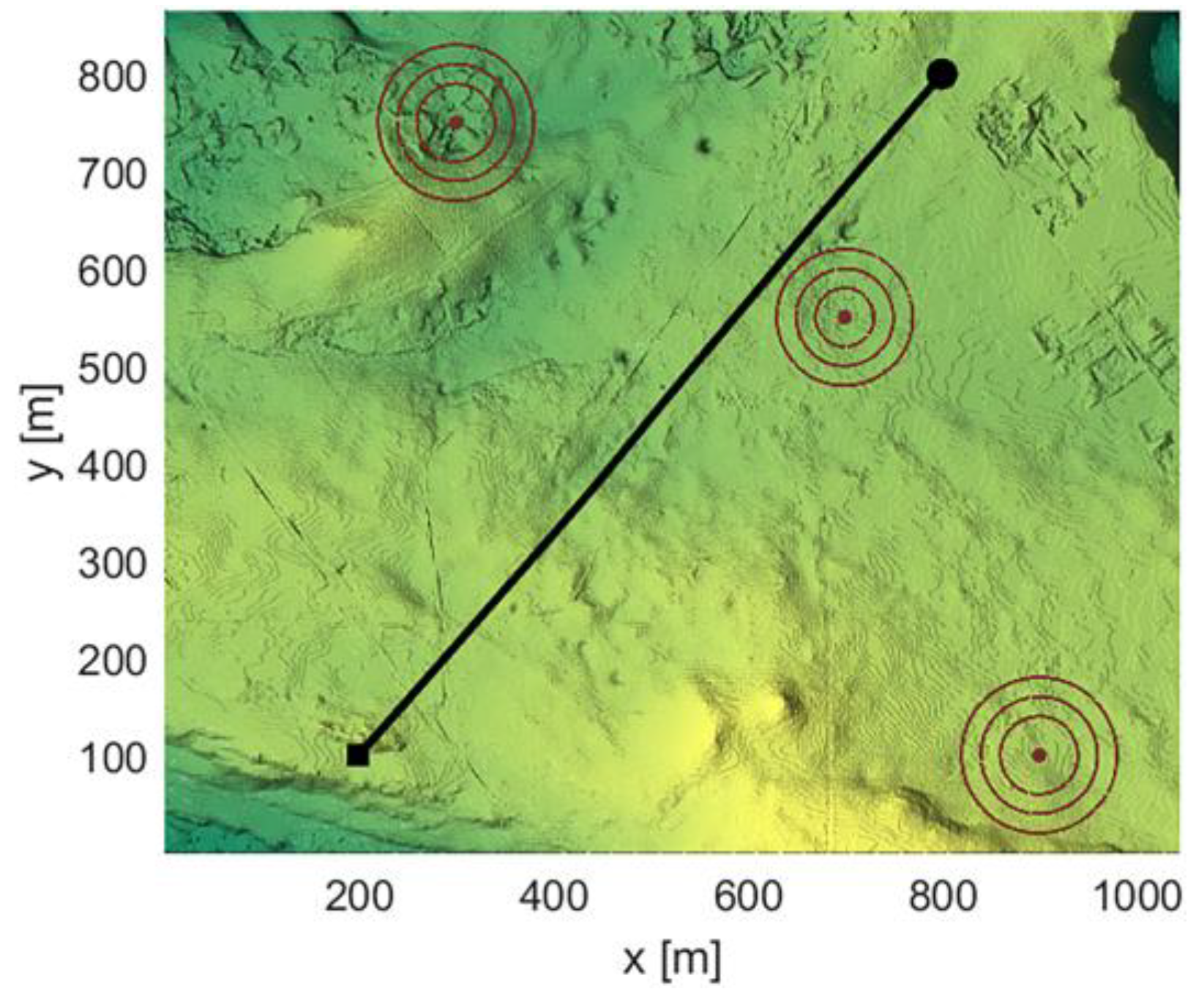
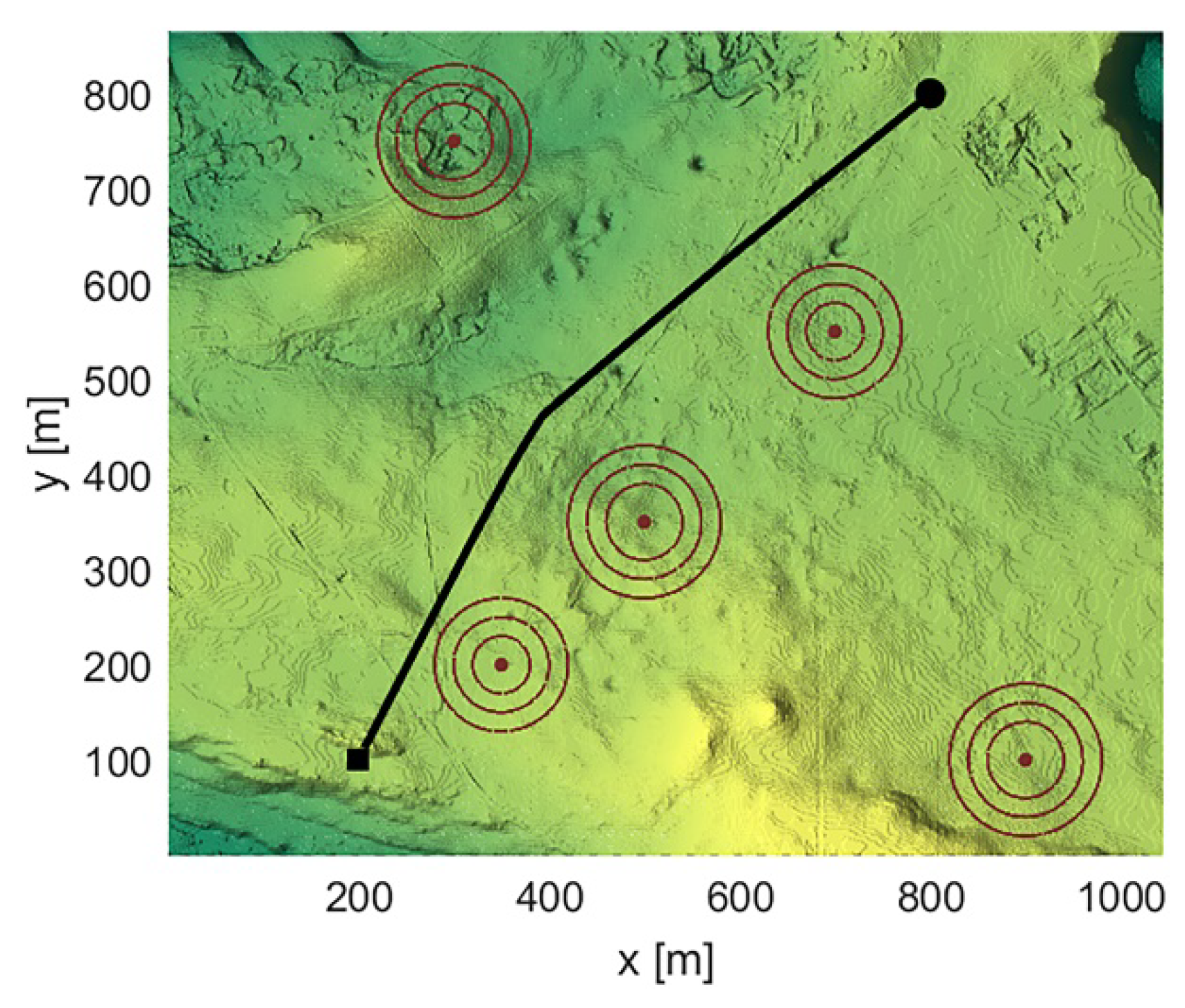
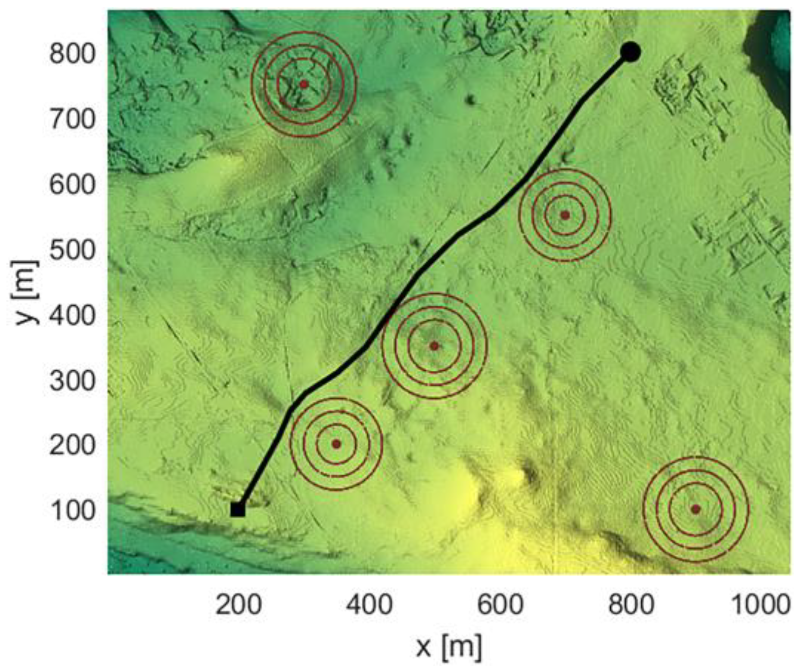
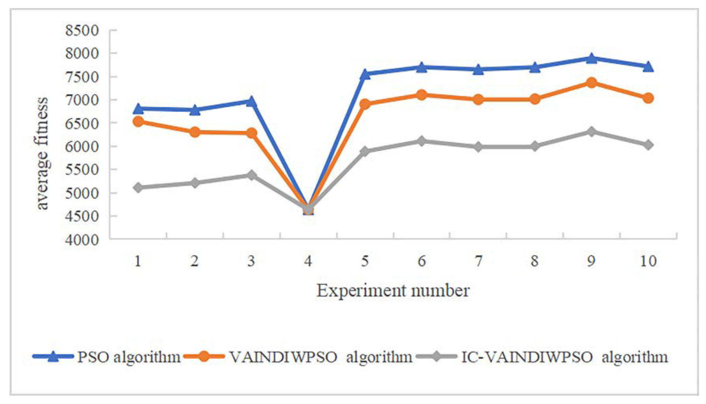
5. Experimental Simulation Analysis
5.1. Experimental Parameters
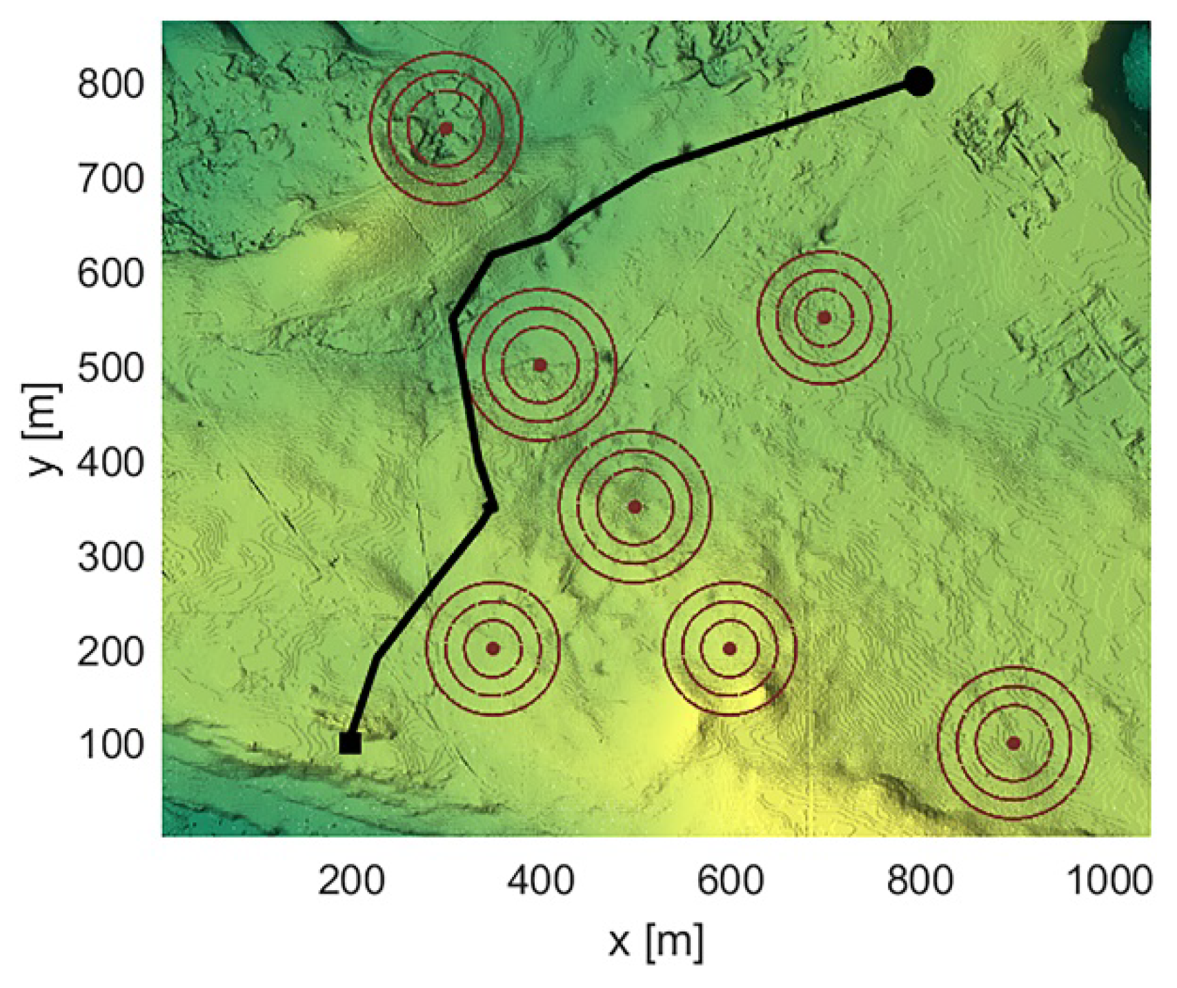
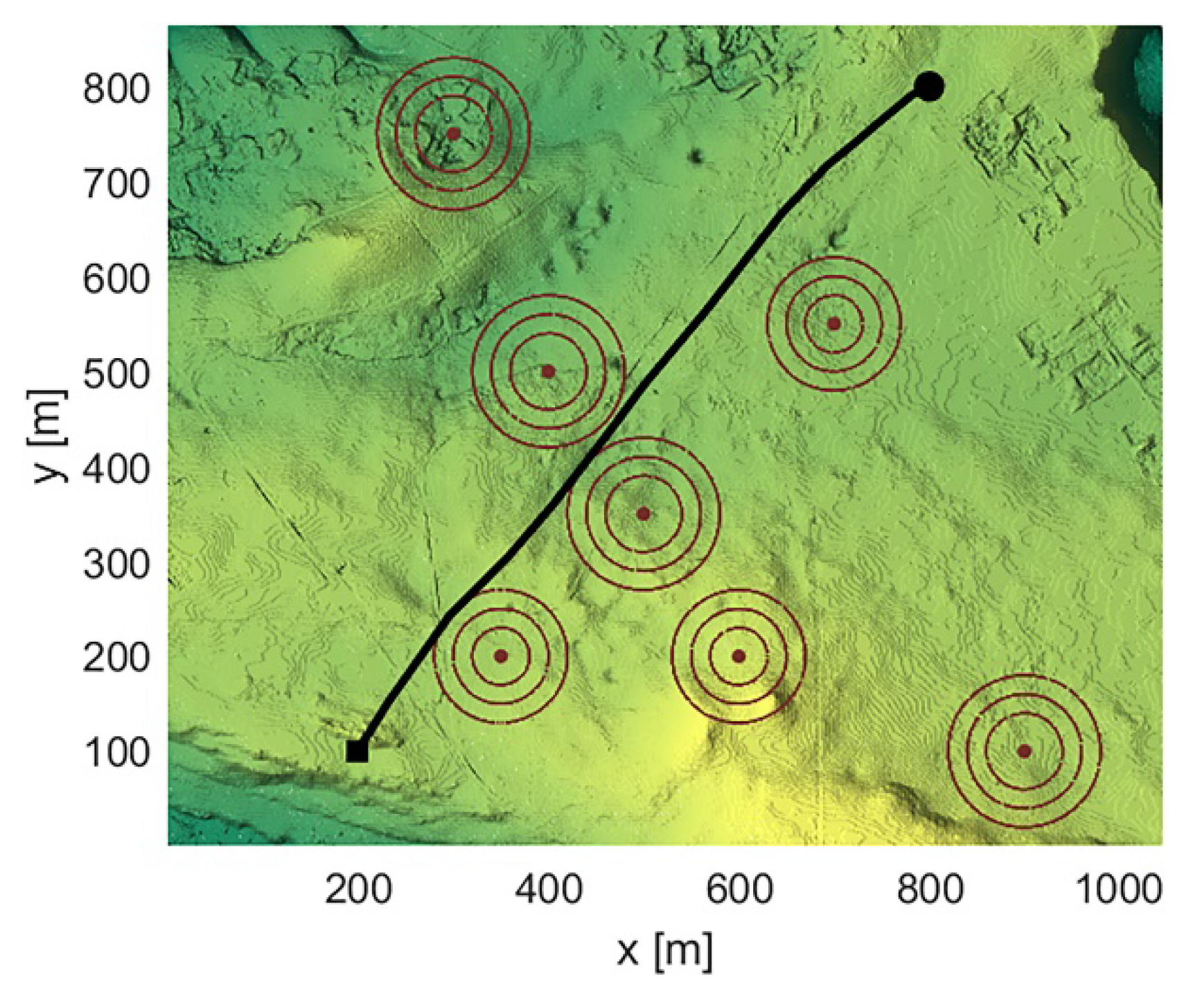
5.2. Analysis of Results
6. Conclusions
Author Contributions
Funding
Institutional Review Board Statement
Informed Consent Statement
Data Availability Statement
Conflicts of Interest
References
- Yu, X.; Li, C.; Zhou, J. A Constrained Differential Evolution Algorithm to Solve UAV Path Planning in Disaster Scenarios. Knowl.-Based Syst. 2020, 204, 106209. [Google Scholar] [CrossRef]
- Zhao, Y.; Zheng, Z.; Liu, Y. Survey on Computational-Intelligence-Based UAV Path Planning. Knowl.-Based Syst. 2018, 158, 54–64. [Google Scholar] [CrossRef]
- Patle, B.K.; Babu, L.G.; Pandey, A.; Parhi, D.R.K.; Jagadeesh, A. A Review: On Path Planning Strategies for Navigation of Mobile Robot. Def. Technol. 2019, 15, 582–606. [Google Scholar] [CrossRef]
- Aggarwal, S.; Kumar, N. Path Planning Techniques for Unmanned Aerial Vehicles: A Review, Solutions, and Challenges. Comput. Commun. 2020, 149, 270–299. [Google Scholar] [CrossRef]
- Sánchez-Ibáñez, J.R.; Pérez-del-Pulgar, C.J.; García-Cerezo, A. Path Planning for Autonomous Mobile Robots: A Review. Sensors 2021, 21, 7898. [Google Scholar] [CrossRef] [PubMed]
- Gul, F.; Mir, I.; Abualigah, L.; Sumari, P.; Forestiero, A. A Consolidated Review of Path Planning and Optimization Techniques: Technical Perspectives and Future Directions. Electronics 2021, 10, 2250. [Google Scholar] [CrossRef]
- Zafar, M.N.; Mohanta, J.C. Methodology for Path Planning and Optimization of Mobile Robots: A Review. Procedia Comput. Sci. 2018, 133, 141–152. [Google Scholar] [CrossRef]
- Zhang, Z.; Wu, J.; Dai, J.; He, C. A Novel Real-Time Penetration Path Planning Algorithm for Stealth UAV in 3D Complex Dynamic Environment. IEEE Access 2020, 8, 122757–122771. [Google Scholar] [CrossRef]
- Kiani, F.; Seyyedabbasi, A.; Aliyev, R.; Gulle, M.U.; Basyildiz, H.; Shah, M.A. Adapted-RRT: Novel Hybrid Method to Solve Three-Dimensional Path Planning Problem Using Sampling and Metaheuristic-Based Algorithms. Neural Comput. Appl. 2021, 33, 15569–15599. [Google Scholar] [CrossRef]
- Ravankar, A.A.; Ravankar, A.; Emaru, T.; Kobayashi, Y. HPPRM: Hybrid Potential Based Probabilistic Roadmap Algorithm for Improved Dynamic Path Planning of Mobile Robots. IEEE Access 2020, 8, 221743–221766. [Google Scholar] [CrossRef]
- Ayawli, B.B.K.; Mei, X.; Shen, M.; Appiah, A.Y.; Kyeremeh, F. Mobile Robot Path Planning in Dynamic Environment Using Voronoi Diagram and Computation Geometry Technique. IEEE Access 2019, 7, 86026–86040. [Google Scholar] [CrossRef]
- Jayaweera, H.M.; Hanoun, S. A Dynamic Artificial Potential Field (D-APF) UAV Path Planning Technique for Following Ground Moving Targets. IEEE Access 2020, 8, 192760–192776. [Google Scholar] [CrossRef]
- Yao, P.; Wang, H.; Su, Z. Cooperative Path Planning with Applications to Target Tracking and Obstacle Avoidance for Multi-UAVs. Aerosp. Sci. Technol. 2016, 54, 10–22. [Google Scholar] [CrossRef]
- Zamani, H.; Nadimi-Shahraki, M.H.; Gandomi, A.H. QANA: Quantum-Based Avian Navigation Optimizer Algorithm. Eng. Appl. Artif. Intell. 2021, 104, 104314. [Google Scholar] [CrossRef]
- Zamani, H.; Nadimi-Shahraki, M.H.; Gandomi, A.H. Starling Murmuration Optimizer: A Novel Bio-Inspired Algorithm for Global and Engineering Optimization. Comput. Methods Appl. Mech. Eng. 2022, 392, 114616. [Google Scholar] [CrossRef]
- Nazarahari, M.; Khanmirza, E.; Doostie, S. Multi-Objective Multi-Robot Path Planning in Continuous Environment Using an Enhanced Genetic Algorithm. Expert Syst. Appl. 2019, 115, 106–120. [Google Scholar] [CrossRef]
- Chen, J.; Ling, F.; Zhang, Y.; You, T.; Liu, Y.; Du, X. Coverage Path Planning of Heterogeneous Unmanned Aerial Vehicles Based on Ant Colony System. Swarm Evol. Comput. 2022, 69, 101005. [Google Scholar] [CrossRef]
- Hu, Y.; Sun, Z.; Cao, L.; Zhang, Y.; Pan, P. Optimization Configuration of Gas Path Sensors Using a Hybrid Method Based on Tabu Search Artificial Bee Colony and Improved Genetic Algorithm in Turbofan Engine. Aerosp. Sci. Technol. 2021, 112, 106642. [Google Scholar] [CrossRef]
- Xia, G.; Han, Z.; Zhao, B.; Wang, X. Local Path Planning for Unmanned Surface Vehicle Collision Avoidance Based on Modified Quantum Particle Swarm Optimization. Complexity 2020, 2020, 3095426. [Google Scholar] [CrossRef]
- Dai, X.; Wei, Y. Application of Improved Moth-Flame Optimization Algorithm for Robot Path Planning. IEEE Access 2021, 9, 105914–105925. [Google Scholar] [CrossRef]
- Wu, P.; Wang, Z.; Jing, H.; Zhao, P. Optimal Time–Jerk Trajectory Planning for Delta Parallel Robot Based on Improved Butterfly Optimization Algorithm. Appl. Sci. 2022, 12, 8145. [Google Scholar] [CrossRef]
- Shao, S.; Peng, Y.; He, C.; Du, Y. Efficient Path Planning for UAV Formation via Comprehensively Improved Particle Swarm Optimization. ISA Trans. 2020, 97, 415–430. [Google Scholar] [CrossRef]
- Song, B.; Wang, Z.; Zou, L. An Improved PSO Algorithm for Smooth Path Planning of Mobile Robots Using Continuous High-Degree Bezier Curve. Appl. Soft Comput. 2021, 100, 106960. [Google Scholar] [CrossRef]
- Wang, Y.; Bai, P.; Liang, X.; Wang, W.; Zhang, J.; Fu, Q. Reconnaissance Mission Conducted by UAV Swarms Based on Distributed PSO Path Planning Algorithms. IEEE Access 2019, 7, 14. [Google Scholar] [CrossRef]
- Huang, C.; Fei, J. UAV Path Planning Based on Particle Swarm Optimization with Global Best Path Competition. Int. J. Patt. Recogn. Artif. Intell. 2018, 32, 1859008. [Google Scholar] [CrossRef]
- Girija, S.; Joshi, A. Fast Hybrid PSO-APF Algorithm for Path Planning in Obstacle Rich Environment. IFAC-PapersOnLine 2019, 52, 25–30. [Google Scholar] [CrossRef]
- Tian, D.; Shi, Z. MPSO: Modified Particle Swarm Optimization and Its Applications. Swarm Evol. Comput. 2018, 41, 49–68. [Google Scholar] [CrossRef]
- Xia, X.; Xing, Y.; Wei, B.; Zhang, Y.; Li, X.; Deng, X.; Gui, L. A Fitness-Based Multi-Role Particle Swarm Optimization. Swarm Evol. Comput. 2019, 44, 349–364. [Google Scholar] [CrossRef]
- Shao, Z.; Yan, F.; Zhou, Z.; Zhu, X. Path Planning for Multi-UAV Formation Rendezvous Based on Distributed Cooperative Particle Swarm Optimization. Appl. Sci. 2019, 9, 2621. [Google Scholar] [CrossRef]
- Jia, L.; Zhao, X. An Improved Particle Swarm Optimization (PSO) Optimized Integral Separation PID and Its Application on Central Position Control System. IEEE Sens. J. 2019, 19, 7064–7071. [Google Scholar] [CrossRef]
- Wang, Z.; Fu, Y.; Song, C.; Zeng, P.; Qiao, L. Power System Anomaly Detection Based on OCSVM Optimized by Improved Particle Swarm Optimization. IEEE Access 2019, 7, 181580–181588. [Google Scholar] [CrossRef]
- Çomak, E. A Particle Swarm Optimizer with Modified Velocity Update and Adaptive Diversity Regulation. Expert Syst. 2019, 36, e12330. [Google Scholar] [CrossRef]
- Lin, C.-J.; Li, T.-H.S.; Kuo, P.-H.; Wang, Y.-H. Integrated Particle Swarm Optimization Algorithm Based Obstacle Avoidance Control Design for Home Service Robot. Comput. Electr. Eng. 2016, 56, 748–762. [Google Scholar] [CrossRef]
- Sabir, Z.; Raja, M.A.Z.; Guirao, J.L.G.; Shoaib, M. A Neuro-Swarming Intelligence-Based Computing for Second Order Singular Periodic Non-Linear Boundary Value Problems. Front. Phys. 2020, 8, 224. [Google Scholar] [CrossRef]
- Umar, M.; Amin, F.; Wahab, H.A.; Baleanu, D. Unsupervised Constrained Neural Network Modeling of Boundary Value Corneal Model for Eye Surgery. Appl. Soft Comput. 2019, 85, 105826. [Google Scholar] [CrossRef]
- Phung, M.D.; Ha, Q.P. Safety-Enhanced UAV Path Planning with Spherical Vector-Based Particle Swarm Optimization. Appl. Soft Comput. 2021, 107, 107376. [Google Scholar] [CrossRef]
- Teng, H.; Ahmad, I.; Msm, A.; Chang, K. 3D Optimal Surveillance Trajectory Planning for Multiple UAVs by Using Particle Swarm Optimization With Surveillance Area Priority. IEEE Access 2020, 8, 86316–86327. [Google Scholar] [CrossRef]
- Wang, B.; Li, S.; Guo, J.; Chen, Q. Car-like Mobile Robot Path Planning in Rough Terrain Using Multi-Objective Particle Swarm Optimization Algorithm. Neurocomputing 2018, 282, 42–51. [Google Scholar] [CrossRef]
- Huang, X.; Li, C.; Chen, H.; An, D. Task Scheduling in Cloud Computing Using Particle Swarm Optimization with Time Varying Inertia Weight Strategies. Clust. Comput. 2020, 23, 1137–1147. [Google Scholar] [CrossRef]
- Kiani, A.T.; Nadeem, M.F.; Ahmed, A.; Khan, I.; Elavarasan, R.M.; Das, N. Optimal PV Parameter Estimation via Double Exponential Function-Based Dynamic Inertia Weight Particle Swarm Optimization. Energies 2020, 13, 4037. [Google Scholar] [CrossRef]
- Tharwat, A.; Elhoseny, M.; Hassanien, A.E.; Gabel, T.; Kumar, A. Intelligent Bézier Curve-Based Path Planning Model Using Chaotic Particle Swarm Optimization Algorithm. Clust. Comput. 2019, 22, 4745–4766. [Google Scholar] [CrossRef]
- Lian, J.; Yu, W.; Xiao, K.; Liu, W. Cubic Spline Interpolation-Based Robot Path Planning Using a Chaotic Adaptive Particle Swarm Optimization Algorithm. Math. Probl. Eng. 2020, 2020, 1849240. [Google Scholar] [CrossRef]
- Masood, F.; Ahmad, J.; Shah, S.A.; Jamal, S.S.; Hussain, I. A Novel Hybrid Secure Image Encryption Based on Julia Set of Fractals and 3D Lorenz Chaotic Map. Entropy 2020, 22, 274. [Google Scholar] [CrossRef] [PubMed]
- Luo, Y.; Zhou, R.; Liu, J.; Cao, Y.; Ding, X. A Parallel Image Encryption Algorithm Based on the Piecewise Linear Chaotic Map and Hyper-Chaotic Map. Nonlinear Dyn. 2018, 93, 1165–1181. [Google Scholar] [CrossRef]
- Wangsheng, F.; Chong, W.; Ruhua, Z. Application of Simulated Annealing Particle Swarm Optimization in Complex Three-Dimensional Path Planning. J. Phys. Conf. Ser. 2021, 1873, 012077. [Google Scholar] [CrossRef]
- Gohari, P.S.; Mohammadi, H.; Taghvaei, S. Using Chaotic Maps for 3D Boundary Surveillance by Quadrotor Robot. Appl. Soft Comput. 2019, 76, 68–77. [Google Scholar] [CrossRef]


| Algorithm | PSO Algorithm | VAINDIWPSO Algorithm | IC-VAINDIWPSO Algorithm |
|---|---|---|---|
| Velocity and position | Equations (10) and (11) | Equations (10) and (11) | Equations (21) and (11) |
| inertia weight | Equation (19) | Equation (19) | |
| update velocity | no | Equation (20) | Equation (20) |
| Chaos initialization | no | no | yes |
| Logistic chaos map | no | no | Equation (22) |
| Parameter Name | Parameter Notation | Parameter Value |
|---|---|---|
| learning factors | c1 = c2 | 1.5 |
| disturbed coefficients | 0.2 | |
| disturbed coefficients | 0.3 | |
| control parameter of the chaotic state | ||
| neighborhood radius | 0.1 |
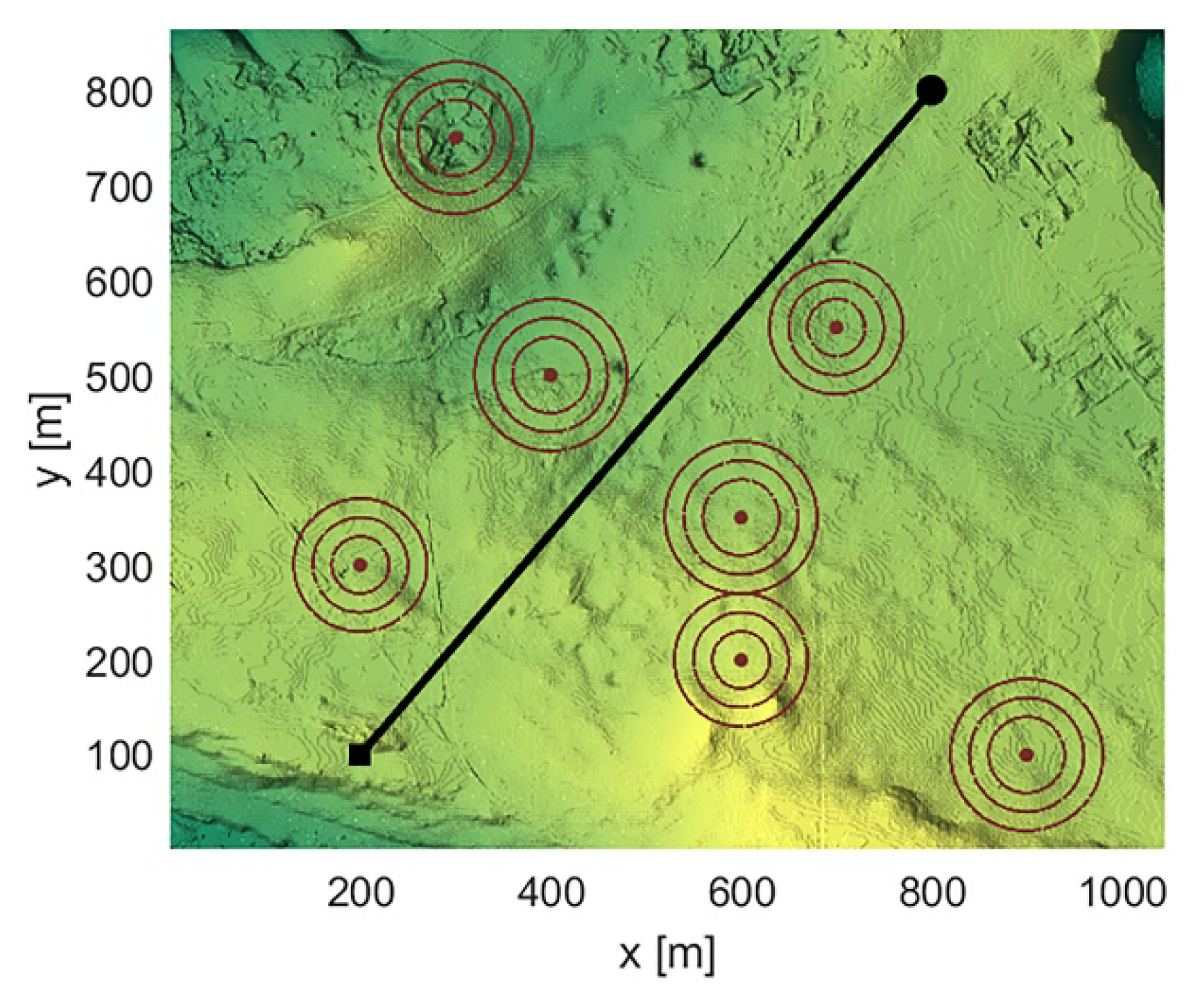
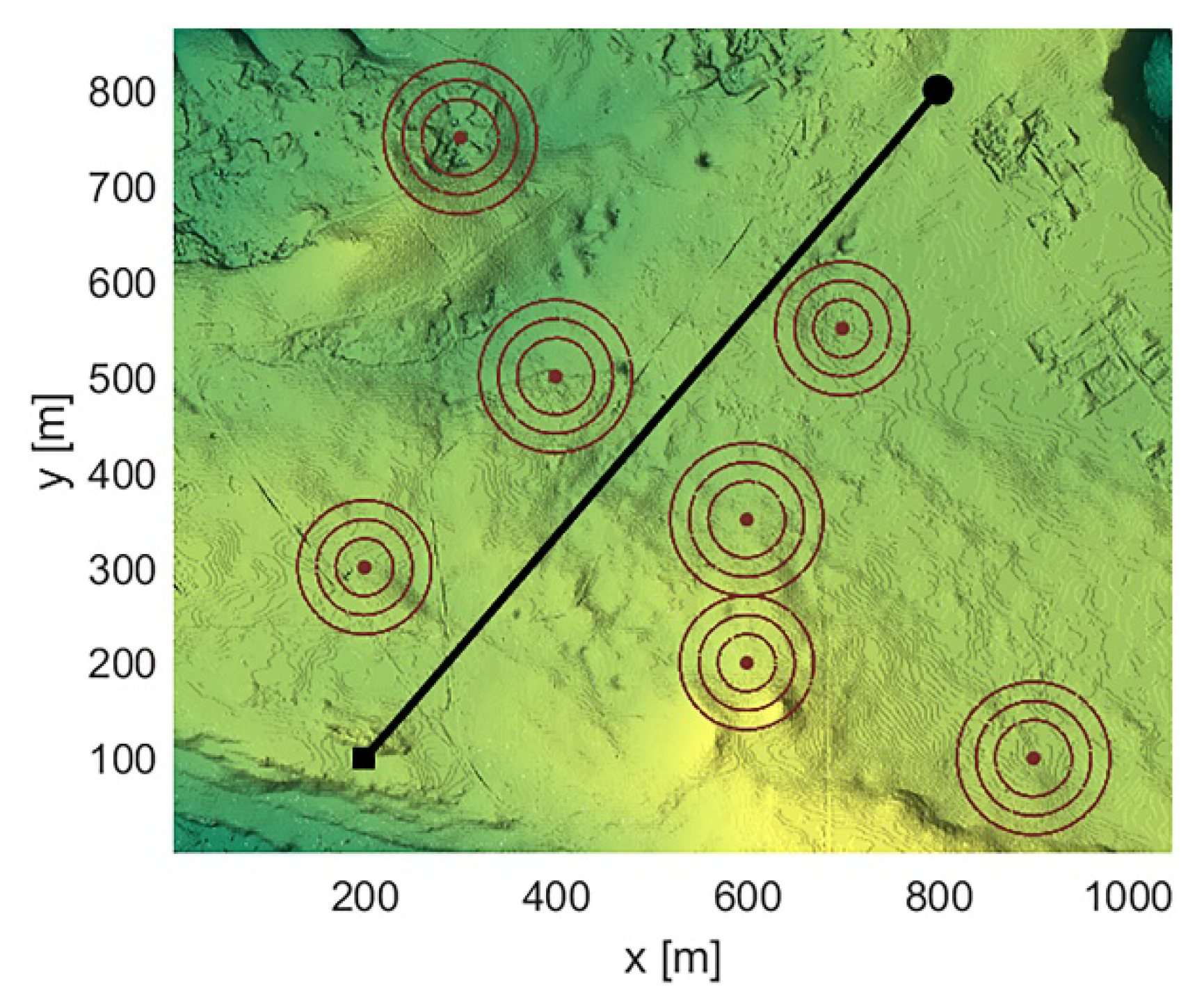
| Threat Number | x | y | z | r | |
|---|---|---|---|---|---|
| Threat Parameter | |||||
| 1 | 900 | 100 | 250 | 80 | |
| 2 | 300 | 750 | 150 | 80 | |
| 3 | 700 | 550 | 150 | 70 | |
| 4 | 350 | 200 | 150 | 70 | |
| 5 | 500 | 350 | 150 | 80 | |
| 6 | 600 | 200 | 150 | 70 | |
| 7 | 400 | 500 | 100 | 80 | |
| Algorithm | Inertia Weight | ω(1) | ωmax | ωmin | ||
|---|---|---|---|---|---|---|
| Parameter | ||||||
| PSO algorithm | 1 | - | - | 0.98 | ||
| VAINDIWPSO algorithm | 1 | 0.9 | 0.4 | - | ||
| IC-VAINDIWPSO algorithm | 1 | 0.9 | 0.4 | - | ||
| Algorithm Name | Initial Population | Number of Iterations | Iterative Convergence Times | Optimal Fitness | Average Fitness | Initialization Runtime/s | Iteration Running Time/s |
|---|---|---|---|---|---|---|---|
| PSO algorithm | 500 | 1000 | 449 | 7256.4168 | 7350.4576 | 4.745 | 130.492 |
| VAINDIWPSO algorithm | 500 | 500 | 250 | 6635.2626 | 6704.6754 | 4.717 | 62.648 |
| IC-VAINDIWPSO algorithm | 1000 | 500 | 20 | 5518.1756 | 5575.7793 | 0.644 | 58.997 |
| IC-VAINDIWPSO algorithm (stop running 50 generations after convergence) | 1000 | 73 | 23 | 5520.1236 | 5579.7346 | 0.654 | 9.424 |
| Algorithm Name | Initial Population | Number of Iterations | Iterative Convergence Times | Optimal Fitness | Average Fitness | Initialization Runtime/s | Iteration Running Time/s |
|---|---|---|---|---|---|---|---|
| PSO algorithm | 500 | 1000 | 153 | 4618.3186 | 4631.182 | 0.167 | 82.169 |
| VAINDIWPSO algorithm | 500 | 500 | 1 | 4637.3815 | 4637.3815 | 0.104 | 46.221 |
| IC-VAINDIWPSO algorithm | 1000 | 500 | 1 | 4637.3815 | 4637.3815 | 0.604 | 43.509 |
| Algorithm Name | Initial Population | Number of Iterations | Iterative Convergence Times | Optimal Fitness | Average Fitness | Initialization Runtime/s | Iteration Running Time/s |
|---|---|---|---|---|---|---|---|
| PSO algorithm | 500 | 1000 | 360 | 5721.9739 | 6058.1241 | 1.134 | 103.802 |
| VAINDIWPSO algorithm | 500 | 500 | 158 | 5422.4877 | 5437.8974 | 0.754 | 53.884 |
| IC-VAINDIWPSO algorithm | 1000 | 500 | 25 | 5196.9241 | 5229.1847 | 0.629 | 51.382 |
| Algorithm | Average Fitness | Iterative Convergence Times |
|---|---|---|
| PSO algorithm | 5781 | 56 |
| QPSO algorithm | 7120 | 761 |
| GA algorithm | 6325 | 224 |
| ABC algorithm | 5325 | 118 |
Publisher’s Note: MDPI stays neutral with regard to jurisdictional claims in published maps and institutional affiliations. |
© 2022 by the authors. Licensee MDPI, Basel, Switzerland. This article is an open access article distributed under the terms and conditions of the Creative Commons Attribution (CC BY) license (https://creativecommons.org/licenses/by/4.0/).
Share and Cite
Chu, H.; Yi, J.; Yang, F. Chaos Particle Swarm Optimization Enhancement Algorithm for UAV Safe Path Planning. Appl. Sci. 2022, 12, 8977. https://doi.org/10.3390/app12188977
Chu H, Yi J, Yang F. Chaos Particle Swarm Optimization Enhancement Algorithm for UAV Safe Path Planning. Applied Sciences. 2022; 12(18):8977. https://doi.org/10.3390/app12188977
Chicago/Turabian StyleChu, Hongyue, Junkai Yi, and Fei Yang. 2022. "Chaos Particle Swarm Optimization Enhancement Algorithm for UAV Safe Path Planning" Applied Sciences 12, no. 18: 8977. https://doi.org/10.3390/app12188977
APA StyleChu, H., Yi, J., & Yang, F. (2022). Chaos Particle Swarm Optimization Enhancement Algorithm for UAV Safe Path Planning. Applied Sciences, 12(18), 8977. https://doi.org/10.3390/app12188977