Missing Well Logs Prediction Based on Hybrid Kernel Extreme Learning Machine Optimized by Bayesian Optimization

Abstract

Geophysical logging is an essential measurement tool in the oil/gas exploration and development field. In practice, predicting missing well logs is an effective way to reduce the exploration expenses. Because of the complexity and heterogeneity of the reservoir, there must be strong nonlinear correlations between the well logs. To improve the accuracy and stability of the missing well logs prediction, a method based on a Bayesian optimized hybrid kernel extreme learning machine (BO-HKELM) algorithm is proposed. Firstly, the LightGBM algorithm is applied to screen out important features related to the missing well logs and reduce the input dimension of the prediction model. Secondly, the hybrid kernel extreme learning machine (HKELM) algorithm is applied to construct the missing well logs prediction model, and the hyperparameters $(C_0,C_1,d,\sigma ,C)$ of the model are optimized by the Bayesian algorithm. Finally, the BO-HKELM model is applied to the prediction of the missing well logs in a block of the Ordos Basin in China. The results show that the RMSE, MAE, and R-square predicted by the BO-HKELM model are 0.0767, 0.0613, and 0.9029, respectively. It can be found that the BO-HKELM model has better regression accuracy and generalization ability, and can estimate missing logs more accurately than the traditional machine learning methods, which provides a promised method for missing well logs estimation.

1. Introduction

In oil/gas exploration, geophysical logging is an effective way of analyzing and describing the subsurface conditions by using physical measurements. The primary measuring items are the electrochemical, acoustic, radioactive, and other geophysical features of the rock formation. In reservoir evaluation, the lithology, physical property, and oil-gas bearing properties of the reservoir can be comprehensively evaluated by using the results of logging data analysis and interpretation. It is essential to merge the various logs and seismic data in order to efficiently develop a reservoir model and decrease the fuzziness of geological interpretation. However, when the logging instrument is faulty, the borehole wall is damaged and collapses occur, which will lead to the loss of logging curves in the working area [1].

It is of great significance to use the logging curves of known intervals to supplement the missing logging curves for subsequent reservoir prediction. Therefore, numerous studies have been carried out in an effort to identify the non-linear correlations between various well logs. According to the investigation, the most frequently used approaches include the empirical model [2,3], the multi-variable linear regression model [4,5] and the traditional machine learning model [6,7]. The empirical model can result in the major deviations because of the strong nonlinear relationship between the reservoir characteristics and missing well logs. The multi-variable linear regression model has the disadvantage of inadequate equation expression. The traditional machine learning model has issues with over-fitting or being trapped in local optimums, as well as the need for sufficient and compact training sample sets [8,9,10]. Therefore, a missing well logs prediction model with excellent computation speed, prediction accuracy and generalization ability is urgently needed.

The extreme learning machine (ELM) is a single hidden layer feedforward neural network with the characteristics of a simple structure and fast learning speed. However, the input weights and the threshold of the hidden layer of the ELM are randomly set, and the appropriate number of the hidden layer is difficult to determine. The kernel extreme learning machine (KELM) uses kernel mapping instead of random mapping, which greatly reduces the complexity of the network and means that the model has better prediction and generalization ability. However, the KELM usually adopts a single kernel function in the application process, which is difficult to adapt to samples with multiple data characteristics [11].

The hybrid kernel extreme learning machine (HKELM) is built by weighing multiple kernel functions to enhance the regression accuracy, which can solve the problem that it is difficult for the KELM with a single kernel function is to obtain the characteristics of a multidimensional sample. However, the parameters of the HKELM model are stochastic, and the training accuracy and time are easily affected by randomness. Therefore, it is necessary to use the optimization algorithm to optimize the hyper-parameters of the HKELM model [12,13,14,15,16]. It has been established that the Bayes optimization algorithm offers exceptional search performance [17]. In this study, a hybrid kernel extreme learning machine, optimized by a Bayesian optimization algorithm (BO-HKELM), is proposed to predict the missing well logs. Furthermore, the BO-HKELM model is applied to two wells (Well A1 and Well A2) in a block of the Ordos Basin in China. It can be found that the BO-HKELM model has higher precision compared to the other models proposed in this research.

2. Principle and Modeling

2.1. Principle of KELM

The ELM is a practical and efficient feedforward neural network. The structure of the ELM network is shown in Figure 1.

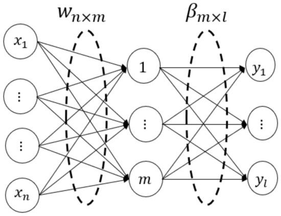
Figure 1. ELM model structure diagram.

In the diagram, $X,Y$ denote the input and output dataset, respectively. ${\mathit{x}}_{\mathit{k}}={\left[\begin{array}{llll}{x}_{\mathrm{k}1}\hfill & x_{\mathrm{k}2}\hfill & \cdots \hfill & x_{kn}\hfill \end{array}\right]}^{\mathrm{T}}$ is the input vector at dimension $n$, and ${\mathit{y}}_{\mathit{k}}={\left[\begin{array}{llll}{y}_{\mathrm{k}1}\hfill & y_{\mathrm{k}2}\hfill & \cdots \hfill & y_{kl}\hfill \end{array}\right]}^{\mathrm{T}}$ is the output vector at dimension $l$. ${\mathit{w}}_j=\left[\begin{array}{llll}{w}_{1j}\hfill & w_{2j}\hfill & \cdots \hfill & w_{nj}\hfill \end{array}\right]$ is the input weight of the node $j$ in the hidden layer, and ${\mathit{\beta }}_j={\left[\begin{array}{llll}{\beta }_{j1}\hfill & {\beta }_{j2}\hfill & \cdots \hfill & {\beta }_{jl}\hfill \end{array}\right]}^{\mathrm{T}}$ is the output weight of the node$j$ in the same hidden layer. $\mathit{b}={\left[\begin{array}{llll}{b}_1\hfill & b_2\hfill & \cdots \hfill & b_m\hfill \end{array}\right]}^{\mathrm{T}}$ is the threshold of the hidden layer. $g\left(x\right)=\frac{1}{1+e^{-x}}$ is the excitation function of the hidden layer. $f_{\mathrm{ELM}}\left({\mathit{x}}_{\mathit{k}}\right)$ is the network output of the ELM, which is expressed as follows:

$$f_{\mathrm{ELM}}\left({\mathit{x}}_k\right)={{\displaystyle \sum }}_{j=1}^m{\mathit{\beta }}_j·g\left({\mathit{w}}_j\cdot {\mathit{x}}_k+b_j\right).$$

(1)

The output matrix $f_{\mathrm{ELM}}\left(X\right)$ can be written as $f_{\mathrm{ELM}}\left(X\right)=\mathit{H}\mathit{\beta }$, where $\mathit{H}$ is the output matrix of the hidden layer:

$$H={\left[\begin{array}{ccc}& & \\ g\left({\mathit{w}}_1·{\mathit{x}}_1+b_1\right)& \cdots & g\left({\mathit{w}}_m·{\mathit{x}}_1+b_m\right)\\ & & \\ g\left({\mathit{w}}_1·{\mathit{x}}_2+b_1\right)& \cdots & g\left({\mathit{w}}_m·{\mathit{x}}_2+b_m\right)\\ & & \\ ⋮& ⋮& ⋮\\ & & \\ g\left({\mathit{w}}_1·{\mathit{x}}_{N^{\prime }}+b_1\right)& \cdots & g\left({\mathit{w}}_m·{\mathit{x}}_{N^{\prime }}+b_m\right)\end{array}\right]}_{N^{\prime }\times m}.$$

(2)

$\mathit{X}$ and $\mathit{Y}$ are both known variables. The input weight matrix $\mathit{W}$ and the threshold $b$ can be randomly given. $\mathit{H}$ can be calculated by Equation (2). The output weight matrix $\mathit{\beta }$ is calculated by the formula $\mathit{\beta }={\mathit{H}}^{+}·\mathit{Y}$, where ${\mathit{H}}^{+}$ is the pseudo-inverse matrix of $\mathit{H}$.

The ELM overcomes the shortcomings of the traditional neural network, such as slow training speed, the overfitting that is prone to occur, and falling into local extremums, but there are still problems, such as difficulty in determining the number of nodes in the hidden layer and the occurrence of overfitting. To address the shortcomings of the ELM, inspired by the kernel function introduced into the support vector machines (SVM), the KELM is proposed in the literature [18], which denotes the mapping from the input to the output of the hidden layer as $h\left(\mathit{X}\right)$.

The kernel matrix is defined as

$${\Omega }_{KELM}\left(\mathit{X}\right)=h\left(\mathit{X}\right)·{\mathit{H}}^T.$$

(3)

The elements at row $i$ and column$j$ of the matrix are shown by the following equation:

$${\Omega }_{KEL{M}_{ij}}\left(x_i,x_j\right)=h\left(x_i\right)·h\left(x_j\right)\triangleq K\left(x_i·x_j\right)$$

(4)

where $K\left(x_i·x_j\right)$ is the kernel function. $f_{KELM}\left(\mathit{X}\right)$ can be estimated by Formula (5), which is described below.

$$\begin{array}{c}{f}_{KELM}\left(\mathit{X}\right)=h\left(\mathit{X}\right)·{\mathit{H}}^T{\left({\mathit{\Omega }}_{KELM}\left(\mathit{X}\right)\right)}^{-1}·\mathit{Y}=\left[K\left(\mathit{X}·{\mathit{x}}_1\right) \cdots K\left(\mathit{X}·{\mathit{x}}_N\right)\right]\times \\ {\left({\mathit{\Omega }}_{KELM}\left(\mathit{X}\right)\right)}^{-1}·\mathit{Y}.\end{array}$$

(5)

After introducing the regularized item, the following equation is used:

$$f_{KELM}\left(\mathit{X}\right)=\left[K\left(\mathit{X}·x_1\right) \cdots K\left(\mathit{X}·x_N\right)\right]\times {\left(\frac{I}{C}+{\mathit{\Omega }}_{KELM}\left(\mathit{X}\right)\right)}^{-1}·\mathit{Y}.$$

(6)

Then, the network output $f_{\mathrm{KELM}}\left(X_k\right)$of the KELM can be written as

$$f_{KELM}\left({\mathit{X}}_k\right)={{\displaystyle \sum }}_{k=1}^n{\Omega }_{KELM}\left(\mathit{X}·{\mathit{x}}_k\right)·{({(\frac{I}{C})}_k+{\Omega }_{KELM}\left(\mathit{X}·{\mathit{x}}_k\right))}^{-1}·{\mathit{Y}}_k$$

(7)

where C is the regular term coefficient. The accuracy of the model increases as the parameter C increases, but overfitting is more likely to happen. Conversely, as C decreases, the generalization ability increases and error-tolerant rate increases, but underfitting is more likely to happen.

2.2. Hybrid Kernel Extreme Learning Machine

By using the kernel function to map the low-dimensional space to the high-dimensional space, the KELM greatly reduces the complexity of the network, and makes the prediction and the generalization ability better [19]. However, even within the same sample, the performance of various kernel functions for prediction is extremely diverse [20], indicating that it is difficult for a single kernel function in the standard KELM algorithm to accommodate diverse logging sample data. Therefore, a hybrid kernel extreme learning machine (HKELM) is proposed. By adding a hybrid kernel, the defect of ELM with a single core can be overcome, and the problem of low prediction accuracy and insufficient generalization ability can be solved.

Based on the synthesis of the characteristics of common kernels and the trade-off between model accuracy and computational complexity, two kinds of kernel functions, polynomial and Gaussian radial basis, are selected to carry out a weighted combination, and the equivalent kernel function, combining the two kinds of kernels, is constructed. The expressions of the two basic kernel functions are shown in Equations (8) and (9), respectively.

Polynomial kernel function can be expressed as

$$K_{\mathit{poly}}\left(\mathit{X},x_k\right)={\left[\left(x_k^T\mathit{X}\right)+C_0\right]}^d,C_0>0$$

(8)

where $C_0$ and $d$ are the parameters of the polynomial kernel function. This kernel function can generally represent the nonlinear mapping of the system.

Gaussian radial basis kernel function can be expressed as

$$K_{RBF}\left(\mathit{X},{\mathit{x}}_k\right)=exp\left(\frac{-\parallel \mathit{X}-{\mathit{x}}_k{\parallel }^2}{2{\sigma }^2}\right)$$

(9)

where σ is the kernel width. This kernel function can generally represent the nonlinearity of the system.

Therefore, the equivalent kernel function used in HKELM algorithm can be expressed as the following equation:

$${\Omega }_{MKELM}\left(\mathit{X},x_k\right)=C_1{K}_{\mathit{poly}}\left(\mathit{X},x_k\right)+C_2{K}_{RBF}\left(\mathit{X},x_k\right)$$

(10)

where $C_1$ and $C_2$ are the weighted coefficients of the kernel function, ranging between (0, 1) and$C_1+C_2=1$. After cancelling out $C_2$,

$${\Omega }_{\mathit{MKELM}}\left(\mathit{X},x_k\right)=C_1·K_{\mathit{poly}}\left(\mathit{X},x_k\right)+\left(1-C_1\right)·K_{RBF}\left(\mathit{X},x_k\right).$$

(11)

After substituting Equation (11) into Equation (7), the output $f_{MKELM}\left({\mathit{x}}_k\right)$ of the proposed HKELM algorithm that integrates the two kernel functions is expressed as

$$\begin{array}{c}{f}_{MKELM}\left(x_k\right)=\\ {{\displaystyle \sum }}_{k=1}^N{\Omega }_{MKELM}\left(\mathit{X}·{\mathit{x}}_k\right)\left\{C_1{\left[\left(x_k^T\mathit{X}\right)+C_0\right]}^d+\right.\left(1-C_1\right){\left.exp\left(\frac{-\parallel \mathit{X}-x_k{\parallel }^2}{2{\sigma }^2}\right)+{\left(\frac{I}{C}\right)}_k\right\}}^{-1}·{\mathit{Y}}_k.\end{array}$$

(12)

The benefits of the global kernel and the local kernel can be combined with the hybrid kernel function of HKELM. So, the HKELM not only has good local search ability but also strengthens the global search ability. Due to the inefficiency in manually determining the hyper-parameter, the HKELM model shoule be optimized by the optimization algorithm.

2.3. Bayesian Optimization Algorithm

The Bayesian optimization algorithm is an intelligent optimization algorithm that can effectively reflect the relationship between variables [21]. The principle of Bayesian optimization is to use Bayes’ theorem to estimate the posterior distribution of the objective function and then select the next combination of hyperparameters to be sampled according to the distribution. This method makes full use of the sampling results of the previous sampling points to improve the shape of the objective function and find the global optimal hyperparameter. One must let $X=x_1,x_2,\dots ,x_n$ be a set of hyperparameter combinations and $f\left(x\right)$ be the objective function of the hyperparameter $x$. The principle of Bayesian optimization is to find $x$, which can be written as

$$x^{\ast }=argmaxf\left(x\right).$$

(13)

The optimization method consists of two parts, a probabilistic surrogate model and a sampling function.

According to Bayes’ theorem, the model parameters are updated in the following equation:

$$p\left(f|D_{1:t}\right)=\frac{p\left(D_{1:t}|f\right)p_{\left(f\right)}}{p\left(D_{1:t}\right)}$$

(14)

where $D_{1:t}=\left\{\left(x_1,f\left(x_1\right)\right),\left(x_2,f\left(x_2\right)\right),\dots ,\left(x_t,f\left(x_t\right)\right)\right\}$ is the sample set; $p\left(D_{1:t}|f\right)$ is the likelihood distribution of $y$; $p\left(f\right)$ is the prior probability model of $f$; $p\left(D_{1:t}\right)$ is the marginal likelihood distribution, and $p\left(f|D_{1:t}\right)$ is the posterior probability model of $f$.

The sampling function is the referenced credential for the Bayesian optimization method to obtain the next sample point in the hyperparameter space. In this research, expected improvement (EI) is used as the sampling function, which is expressed as

$$\left\{\begin{array}{c}\alpha \left(x\right)=\left[\mu \left(x\right)-q^{+}\right]\varnothing \left(Z\right)+\sigma \left(x\right)\phi \left(z\right)\\ x_{t+1}=argmaxf\left(x\right)\end{array}\right.$$

(15)

where $\alpha \left(x\right)$ is the objective function; $\mu \left(x\right)$ is the mean value; $\sigma \left(x\right)$ is the standard deviation value; $q^{+}$ is the maximum value of the current objective function; $\varnothing \left(Z\right)$ is the cumulative distribution function of the Gaussian distribution; $\phi \left(z\right)$ is the probability density function of the distribution, and $x_{t+1}$ is the hyperparameter of the evaluation.

3. Process of Predicting Missing Logging Curves Based on BO-HKELM

In this research, the specific steps for optimizing the parameters ($C_0,C_1,d,\sigma ,C$) in HKELM by the Bayesian algorithm are as follows.

In Step 1, one must divide the input logging dataset into a training set and test set, and normalize the data to (0, 1) using the max–min normalization method. The expression of the max–min normalization method is as follows:

$$x^{\prime }=\frac{x-x_{min}}{x_{max}-x_{min}}$$

(16)

where $x$ is the actual vector. $x_{max}$ and $x_{min}$ are the maximum and minimum values of the vector x, respectively. $x^{\prime }$ is the normalized vector.

In Step 2, one must initialize the model, including the value range, the initial population, the maximum iterations, and the upper accuracy setting of the parameters ($C_0,C_1,d,\sigma ,C$) in HKELM.

In Step 3, one must randomly select a group from the initial population as the initial solution.

In Step 4, one must construct the probability distribution function of the Bayesian network through the Gaussian process, and establish or update an objective function model. The objective function is the root mean square error (RMSE), which is expressed as

$$RMSE=\sqrt{\frac{1}{N}{{\displaystyle \sum }}_{i=1}^N{\left(y_k-{\widehat{y}}_k\right)}^2}$$

(17)

where $y_k$ is the true value, and ${\widehat{y}}_k$is the predicted value of HKELM.

In Step 5, one must determine the position of the next cycle parameter combination according to the acquisition function.

In Step 6, one must calculate the probability value of the parameter combination and update the population distribution.

In Step 7, one must determine whether the resulting combination of parameters satisfies the condition; if so, output the optimum results of $C_0,C_1,d,\sigma ,C$. If not, one must return to Step 4 and repeat the experiment until the condition is satisfied or the maximum number of iterations is reached.

In Step 8, one must apply the optimum parameter combination $(C_0,C_1, d,\sigma ,C)$ to the missing well logs estimation of the HKELM.

In Step 9, one must evaluate the accuracy of the optimized prediction results using the test sample set, and compare the changes in accuracy before and after optimization.

The optimization process is shown in Figure 2.

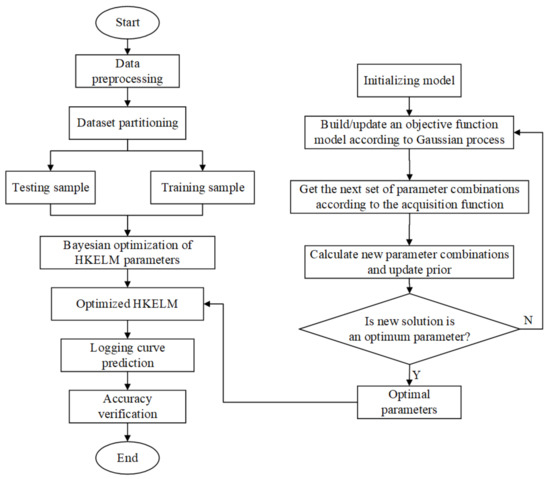
Figure 2. Flow chart of optimizing parameters of HKEM based on Bayesian algorithm.

4. Practical Application and Result Analysis

4.1. Data Preparation

In this research, two exploration wells located in a block of the Ordos Basin in China are studied. The Ordos Basin has the character of stable depression tectonic basin, with the metamorphic crystalline rock series of Archaea and Middle Proterozoic as the rigid sedimentary basement, overlying the platform type sedimentary caps of Middle and Upper Proterozoic, Early Paleozoic, Late Paleozoic and Mesozoic. The Mesozoic is a single fluvial and lacustrine facies terrine detrital coal-bearing sedimentary formation, characterized by the large thickness and wide distribution of lacustrine deltas in the Triassic Yanchang Formation, which is one of the most important oil-gas enrichment horizons in Ordos Basin.

We designate the two wells as Well A1 and Well A2, respectively, to maintain the privacy of well information. Additionally, since the petrophysical logs are primarily found in the intervals of the oil/gas reservoirs, the interest interval of the two selected wells is focused on the Upper Triassic Yanchang Formation. The log graphs of Well A1 and Well A2 are shown in Figure 3 and Figure 4, respectively. The petrophysical logs in the studied interval of the two wells are DEPTH, caliper (CAL), neutron porosity (NPHI), density (RHOB), gamma ray (GR), acoustic time difference (DT), and true resistivity (RT). In addition, DEPTH, CAL, NPHI, RHOB, GR, DT, and RT can be used to measure depth, diameter, porosity, density, shale content, acoustic time difference, and true resistivity of the borehole surrounding rock, respectively. The response of the logging sequence is a comprehensive reflection of the lithology, physical property, electrical property and oil-gas property of the corresponding underground formation. Caliper logging is used to indicate hole expansion and aid in lithology identification and borehole correction. Generally, the oil and gas have the physical characteristics of lower density, higher acoustic time difference and higher resistivity compared with water. In a conventional reservoir, oil and gas are usually filled in the pores and fractures of the formation. Meanwhile, the lower the mud content in the formation, the higher the porosity. Therefore, in the conventional reservoir, the logging response characteristics of high porosity, high acoustic time difference, high resistivity, low mud content and low density may indicate hydrocarbon enrichment. In this research, we suppose the RHOB log is missing and forecast the “missing” RHOB curve using other logging data by BO-HKELM.

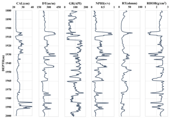
Figure 3. Well logging graph of Well A1 in the studied interval.

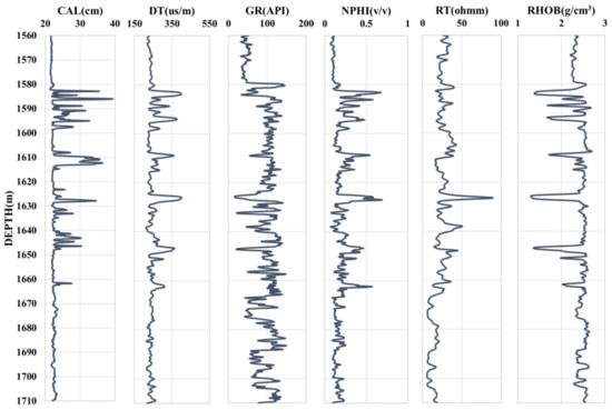
Figure 4. Well logging graph of Well A2 in the studied interval.

The statistical properties of the two selected wells are presented in Table 1. There are 1601 and 1202 data points in Well A1 and Well A2, respectively.

Table 1. Statistical characteristics of Well A1 and Well A2 in the studied interval.

Well Name	Index	Petrophysical Well Logs
		DEPTH (m)	CAL (cm)	DT (μs/m)	GR (API)	NPHI (v/v)	RT (ohmm)	RHOB (g/cm3)
Well A1	Min	1880.00	21.95	187.38	14.97	0.03	6.41	1.21
	25%	1910.00	23.11	231.29	53.00	0.17	16.71	2.24
	50%	1940.00	24.53	237.78	86.11	0.20	27.23	2.31
	Mean	1940.00	25.03	250.97	93.53	0.27	30.44	2.29
	75%	1970.03	26.21	260.20	132.76	0.34	43.07	2.47
	Max	2000.00	41.88	407.97	212.32	0.92	70.84	2.70
Well A2	Min	1560.00	21.36	210.12	15.63	0.07	5.56	1.30
	25%	1597.46	22.11	230.24	65.50	0.12	16.75	2.34
	50%	1635.00	22.40	238.13	99.62	0.17	21.78	2.48
	Mean	1635.00	23.17	249.17	91.19	0.19	22.73	2.39
	75%	1672.53	22.87	251.64	114.39	0.23	28.39	2.54
	Max	1710.00	39.43	400.92	149.03	0.69	89.92	2.70

4.2. Feature Analysis

In this research, the decision tree-based distributed gradient lifting framework (LightGBM) is used to assess the importance of the features. LightGBM is a lightweight framework of the gradient boosting decision tree algorithm. It uses decision tree iterative training to obtain the optimal model, which has the advantages of excellent training effects and difficulty to over-fit. Compared with the extreme gradient boosting, LightGBM uses a gradient-based one-side sampling algorithm to accelerate the training speed of the model, without compromising accuracy [22].

Six parameters, including DEPTH, CAL, NPHI, GR, DT, and RT, from Well A1 are input into the LightGBM model to obtain the influence of each parameter on RHOB and order the characteristic importance. The quantitative results are shown in Table 2:

Table 2. Importance scores of the parameters based on the LightGBM model.

Rank	Feature	Score
1	DT	865
2	NPHI	661
3	CAL	594
4	GR	466
5	RT	448
6	DEPTH	429

The features are added one by one in descending order of relevance to the ordinary model (KELM) in order to choose the significant sample features. Figure 5 displays the change curve of model errors (RMSE) that is determined by the comparison test. The declining trend of RMSE shows a substantial change when the model contains four inputs, as shown in Figure 5. Therefore, to reduce the computational complexity and the time duration, a model with four inputs is applied to estimate the “missing” RHOB logs. The four input variables are DT, NPHI, CAL, and GR.

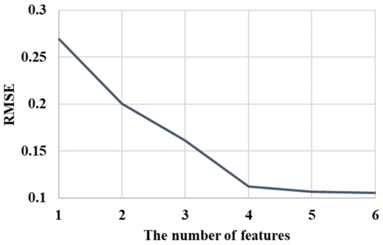
Figure 5. RMSE variation curve of different characteristic numbers.

4.3. Optimization of Algorithm Parameters

In this research, it is assumed that Well A1 in the studied interval has the complete RHOB curve, and the RHOB curve of Well A1 is used as the training set to establish the ELM, KELM, HKELM, and BO-HKELM models. The “missing” RHOB curve of Well A2 in the corresponding interval is predicted.

The Bayesian optimization algorithm introduced in Section 2.3 is used to optimize five parameters in the BO-HKELM model, such as the polynomial kernel function parameters $C_0$ and $d$, the Gaussian radial basis kernel function width $\sigma$, the kernel weighting coefficient $C_1$, and the the regular term coefficient $C$. These five tuning parameters control the developed HKELM’s capacity for prediction, learning, and generalization. To acquire the optimized hyperparameters of the HKELM model, all of the values for each parameter ($C_0,C_1,d,\sigma ,C$) are placed in five distinct vectors. The goal of the optimization procedure is to compare the different parameter combinations and select the optimal ($C_0,C_1,d,\sigma ,C$) values with the lowest cost function. The fitness (RMSE) reduction rate in the training phase of HKELM in Well A1 is shown in Figure 6.

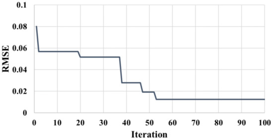
Figure 6. The fitness reduction rate in different iterations of Bayesian optimization algorithm for training HKELM.

It can be observed that the fitness value decreases sharply in the optimization process of the first 53 generations, and the best fitness value is found around the 50th generation, and then the fitness value remains basically unchanged. The parameter optimization results of the Bayesian algorithm are shown in Table 3.

Table 3. The optimal parameters optimized by Bayesian algorithm in Well A1.

BO-HKELM	${\mathit{C}}_0$	${\mathit{C}}_1$	$\mathit{d}$	$\mathit{\sigma }$	$\mathit{C}$
Trained by Well A1	21.43	0.24	2	69.03	86.03

4.4. Comparative Analysis of Model Prediction Effect

The quantitative prediction results are shown in Table 4. It can be observed that the KELM (radial basis function, RBF) model has better prediction accuracy than the ELM model, indicating that the addition of the kernel function can improve the prediction effect. We can also observe that the prediction accuracy of the HKELM model is better than that of KELM (RBF) model, which indicates that the addition of a hybrid kernel function can also improve the prediction ability. The quantitative prediction results show the higher accuracy of the BO-HKELM model compared to the ELM, KELM (RBF) and HKELM models. It can be interpreted that the BO-HKELM model adopts the hybrid kernel and the Bayesian optimization algorithm to obtain the optimal parameters, which improves the generalization ability and prediction accuracy.

Table 4. The outcomes of estimating RHOB in Well A2 using the trained models from Well A1.

Model	RMSE	MAE	R-Square
ELM	0.1133	0.0798	0.7916
KELM	0.1055	0.0638	0.8178
HKELM	0. 0901	0.0623	0.8874
BO-HKELM	0.0767	0.0613	0.9029

The comparison between measured and estimated RHOB in Well A2 by the trained models (ELM, KELM (RBF), HKELM, and BO-HKELM) in Well A1 is shown in Figure 7. It can be observed that when the change in the logging curve is relatively stable, the output results of the BO-HKELM model and other models show little difference. Meanwhile, when the log curve has a local abrupt change (the green frame), the prediction result of the BO-HKELM model is closer to the measured value than the other models, indicating that the BO-HKELM model can extract the spatial characteristics of the log curve more. Therefore, compared with the ordinary machine learning model, the BO-HKELM model is more suitable for missing logging curve prediction.

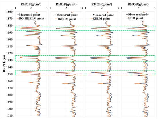
Figure 7. Visual results of the RHOB prediction results of Well A2.

The cross-plots of original RHOB vs predicted RHOB using ELM, KELM (RBF), HKELM, and BO-HKELM in Well A2 are shown in Figure 8. It can be observed that the predicted results of BO-HKELM are closer to the actual RHOB than the other models, indicating that the BO-HKELM is better than other models in fitting multiple local details of DTS. In addition, it can be observed from the quantitative prediction results in Table 4 that compared with other models, the BO-HKELM model has lower errors and higher accuracy, which also reflects its advantages.

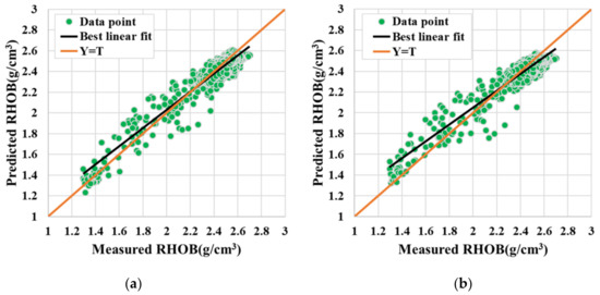
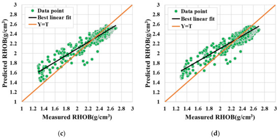
Figure 8. (a) BO-HKELM, (b) HKELM, (c) KELM, (d) ELM. The cross plot of measured RHOB versus the predicted one using BO-HKELM, HKELM, KELM, and ELM at testing phases in Well A2.

To compare the prediction ability of the BO-HKELM model and other models in the case of local abrupt changes in the logging curves, the prediction results of Well A2 are locally amplified and analyzed. The comparison outputs are shown in Figure 9. The black curve is the measured RHOB, and the red, orange, purple and green curves represent the prediction results of BO-HKELM, HKELM, KELM and ELM, respectively. It can be found from the Figure 9 that when the logging curve smoothly changes, the output results of the BO-HKELM model and other models show little difference. While the log curve has the local mutation, the prediction result of the BO-HKELM model is closer to the measured value than other models. The reason is that the BO-HKELM model adds a hybrid kernel function and adopts a Bayesian algorithm to optimize the hyper-parameters, which can fully extract the spatial characteristics of the log curve and enhance the prediction ability of the model.

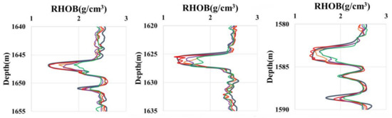
Figure 9. Local enlarged display of prediction results in Well A2.

In conclusion, the BO-HKELM model proposed in this research has an excellent prediction effect overall and reveals a local abrupt change in the logging curves, clearly demonstrating its advantages in predicting the missing well logs.

5. Conclusions

A missing well logs prediction method based on the hybrid BO-HKELM algorithm is proposed in this research by using the common petrophysical data from a field of the Ordos Basin in China. The ELM, KELM (RBF), and HKELM algorithms are used to assess the precision and generalizability of the obtained model. The LightGBM algorithm is applied in conjunction with the original model (HKELM) to show that modeling errors decrease as the number of estimator model inputs increase; however, the trend is only minimal after four input variables. Thus, it can be concluded that the variables DT, NPHI, CAL, and GR are the appropriate modeling inputs. In comparison to the other models studied in this research, the BO-HKELM model has the highest accuracy (R-square: 0.9029) and the lowest error (RMSE: 0.0767 and MAE: 0.0613). In addition, the BO-HKELM model outperforms other models in terms of fitting different local logging curve features, and it is better at rebuilding local curve characteristics when the reservoir curve exhibits a local mutation. The reason is that the BO-HKELM model incorporates a hybrid kernel function and uses a Bayesian algorithm to optimize the parameter weights, which may extract the spatial properties of the log curve more effectively and improve the model’s predictive ability. Therefore, it can be confidently stated that the BO-HKELM model has higher precision and is much better suited for missing well logs prediction, compared to the other models studied in this research.

References

- Sun, Y.Z.; Huang, J. Application of multi-task deep learning in reservoir shear wave prediction. Prog. Geophys. 2021, 36, 799–809. [Google Scholar]
- Gardner, G.; Gardner, L.W.; Gregory, A.R. Formation velocity and density; the diagnostic basics for stratigraphic traps. Geophysics 1974, 39, 770–780. [Google Scholar] [CrossRef]
- Smith, J.H. A Method for Calculating Pseudo Sonics from E-Logs in a Clastic Geologic Setting. Gcags Transactions 2007, 57, 1–4. [Google Scholar]
- Wang, J.; Liang, L.; Qiang, D.; Tian, P.; Tan, W. Research and application of reconstructing logging curve based on multi-source regression model. Lithologic Reserv. 2016, 28, 113–120. [Google Scholar]
- Liao, H.M. Multivariate regression method for correcting the influence of expanding diameter on acoustic curve of density curve. Geophys. Geochem. Explor. 2014, 38, 174–179. [Google Scholar]
- Banchs, R.; Jiménez, J.R.; Pino, E.D. Nonlinear estimation of missing logs from existing well log data. In Proceedings of the 2001 SEG Annual Meeting, San Antonio, TX, USA, 2–6 September 2001. [Google Scholar]
- Salehi, M.M.; Rahmati, M.; Karimnezhad, M.; Omidvar, P. Estimation of the non records logs from existing logs using artificial neural networks. Egypt. J. Pet. 2016, 26, 957–968. [Google Scholar] [CrossRef]
- Ramachandram, D.; Taylor, G.W. Deep Multimodal Learning: A Survey on Recent Advances and Trends. IEEE Signal Process. Mag. 2017, 34, 96–108. [Google Scholar] [CrossRef]
- Zhang, Q.; Yang, L.T.; Chen, Z.; Li, P. A survey on deep learning for big data. Inf. Fusion 2018, 42, 146–157. [Google Scholar] [CrossRef]
- Jian, H.; Chenghui, L.; Zhimin, C.; Haiwei, M. Integration of deep neural networks and ensemble learning machines for missing well logs estimation. Flow Meas. Instrum. 2020, 73, 101748. [Google Scholar] [CrossRef]
- Lin, T.; Cai, R.; Zhang, L.; Yang, X.; Liu, G.; Liao, W. Prediction intervals forecasts of wind power based on IBA-KELM. Renew. Energy Resour. 2018, 36, 1092–1097. [Google Scholar]
- Abdullah, M.; Rashid, T.A. Fitness Dependent Optimizer: Inspired by the Bee Swarming Reproductive Process. IEEE Access 2019, 7, 43473–43486. [Google Scholar] [CrossRef]
- Cheng, R.; Jin, Y. A Competitive Swarm Optimizer for Large Scale Optimization. IEEE Trans. Cybern. 2015, 45, 191–204. [Google Scholar] [CrossRef] [PubMed]
- Zhao, W.; Wang, L.; Zhang, Z. Supply-Demand-Based Optimization: A Novel Economics-Inspired Algorithm for Global Optimization. IEEE Access 2019, 7, 73182–73206. [Google Scholar] [CrossRef]
- Shabani, A.; Asgarian, B.; Salido, M.A.; Gharebaghi, S.A. Search and Rescue optimization algorithm: A new optimization method for solving constrained engineering optimization problems. Expert Syst. Appl. 2020, 161, 113698. [Google Scholar] [CrossRef]
- Das, B.; Mukherjee, V.; Das, D. Student psychology based optimization algorithm: A new population based optimization algorithm for solving optimization problems—ScienceDirect. Adv. Eng. Softw. 2020, 146, 102804. [Google Scholar] [CrossRef]
- Sultana, N.; Hossain, S.; Almuhaini, S.H.; Düştegör, D. Bayesian Optimization Algorithm-Based Statistical and Machine Learning Approaches for Forecasting Short-Term Electricity Demand. Energies 2022, 15, 3425. [Google Scholar] [CrossRef]
- Huang, G.B.; Zhou, H.; Ding, X.; Zhang, R. Extreme Learning Machine for Regression and Multiclass Classification. IEEE Trans. Syst. Man Cybern. Part B 2012, 42, 513–529. [Google Scholar] [CrossRef] [PubMed]
- Heidari, A.A.; Rahim, A.A.; Chen, H. Efficient boosted grey wolf optimizers for global search and kernel extreme learning machine training. Appl. Soft Comput. 2019, 81, 105521. [Google Scholar] [CrossRef]
- Chao, Z.; Yin, K.; Cao, Y.; Intrieri, E.; Ahmed, B.; Catani, F. Displacement prediction of step-like landslide by applying a novel kernel extreme learning machine method. Landslides 2018, 15, 2211–2225. [Google Scholar]
- Pelikan, M. Bayesian Optimization Algorithm: From Single Level to Hierarchy. Master’s Thesis, University of Illinois at Urbana-Champaign, Champaign, IL, USA, 2002. [Google Scholar]
- Wang, X.; Zhang, G.; Lou, S.; Liang, S.; Sheng, X. Two-round feature selection combining with LightGBM classifier for disturbance event recognition in phase-sensitive OTDR system. Infrared Phys. Technol. 2022, 123, 104191. [Google Scholar] [CrossRef]
Publisher’s Note: MDPI stays neutral with regard to jurisdictional claims in published maps and institutional affiliations. |
© 2022 by the authors. Licensee MDPI, Basel, Switzerland. This article is an open access article distributed under the terms and conditions of the Creative Commons Attribution (CC BY) license (https://creativecommons.org/licenses/by/4.0/).