Abstract
In the present paper, the fluid flow and heat transfer of a nanofluid are numerically investigated. More specifically, reference is made to a nanofluid, described by means of Buongiorno’s model, subjected to Couette flow. The considered domain consists of a channel that displays a cavity shortly after the inlet section. The transport model for the nanofluid, that is the mass conservation, momentum, and nanoparticles equation, is written in a dimensionless form and solved by employing the software package Comsol Multiphysics. Many ideas emerged from this work: the visualization of the velocity stream function, the dimensionless temperature, and nanoparticle concentration fields are provided, as a function of the governing parameters: Reynolds, Peclet, Lewis, Brownian diffusivity number, and thermophoretic diffusivity number. Concerning the nanofluid typical effects, the thermophoretic diffusion seems to affect the solution much more than the Brownian diffusion. The Nusselt number on the upper wall is calculated as well, and the results show that it proves to be, in most of the considered cases, an increasing function of the Reynolds number. Moreover, concerning the Nusselt number, the Brownian diffusion effects are shown to be negligible.
1. Introduction
The term “nanofluid” was first coined by Choi and Eastman [1,2] in 1995. Originally, the term described nanometer-sized copper particles dispersed in water to improve their thermal conductivity. Today, a nanofluid can be more accurately intended as an engineered colloidal suspension of nanoparticles into a base fluid. Nanofluids have shown a promising future as thermal fluids for various heat transfer applications [3]: in solar collectors [4,5], to enhance the heat-transfer coefficient of solar water heaters or to improve the capacity of thermal energy storage systems; and in the area of refrigeration, to enhance the performance of refrigeration systems. Later, many authors (see for example refs. [6,7,8,9,10]) studied the nanofluid flow and discussed their heat transfer performance. In the literature, a widely employed approach to describe the features of a nanofluid is the so-called Buongiorno model, which relies on the assumptions: (i) the flow is incompressible, (ii) there are no chemical reactions at nanofluids, (iii) external forces are negligible, (iv) the mixture is considered to be diluted, (v) viscous dissipation is negligible, (vi) radiation heat transfer is negligible, (vii) nanoparticles and base fluid are located in thermal equilibrium.
More specifically, Buongiorno presented the following seven mechanisms of slip between nanoparticle and fluid [11]: Inertia, Brownian diffusion, Thermophoresis, Diffusiophoresis, Magnus effect, Fluid Drainage, and Gravity settling. It is worth mentioning that the above-mentioned phenomena can produce a relative velocity between the base fluid and nanoparticles, that is, water. He also suggested a two-component four-equation nonhomogeneous equilibrium model for three basic equations: mass, momentum, and heat transfer. Furthermore, a comparison of length scales and the nanoparticle turbulent eddy time demonstrated that, in the presence of turbulent eddies, the nanoparticle moves with the base fluid homogeneously. As a consequence, the turbulence intensity effect is also double. The presence of turbulence in the flow, which prevents the agglomeration of particles, decreases the discrepancy between experimental and numerical results. Hence, the results obtained from an analysis of Buongiorno’s two-phase model are likely to be more accurate.
In this context, Azimikivi H. et al. [12] recount the effects of the rib shape with constant height, width and pitch, and nanoparticle diameter on natural convection heat transfer of low turbulence flow of AL2O3-water nanofluid inside a square cavity based on Buongiorno’s model. The steady Cu-water nanofluid flow in the presence of a magnetic field has been numerically investigated by Rawat S.K. et al. [13] under the effects of mixed convection, thermal radiation, and chemical reaction. Besides this, the modeled nanofluid problem is characterized by a single-phase nanofluid model (i.e., Tiwari and Das’s model) and a two-phase mixture nanofluid model (i.e., Buongiorno’s model) together with the Cattaneo–Christov Double diffusion model.
In addition, according to Buongiorno’s model, many papers have examined the convection of a nanofluid in a cavity or in a channel with an embedded cavity. In this regard, the forced convection heat transfer of a nanofluid in a channel has been widely investigated in refs. [14,15], while the mixed convection of a nanofluid (with various types of nanoparticles) in an open cavity has been pointed out by Mehrez et al. in ref. [16]. The single phase model has been employed to investigate the Couette forced convection of a nanofluid in ref. [17]: the governing PDEs are reduced to ODEs using a similarity transformation, and then analytically solved. The recent literature has paid attention, especially, to mixed and free convention, or, concerning forced convection, to the presence of MHD effects, as in refs. [18,19,20]. On the contrary, recently, the analysis of vortex formation in the case of laminar flow of a Newtonian fluid, flowing in a duct with an embedded cavity has been studied in ref. [21], where a brief analysis of the recent literature on the vortex formation in cavities is reported as well. In this context, the motivation in the current work is that flow of nanofluid over a channel/embedded cavity has been extensively discussed in the past by many authors, yet none of them made an attempt to combine the forced convection of a two-phase mixture of nanofluid with Couette flow.
More in detail, in the present paper, attention is paid to the Couette laminar flow of a nanofluid in a channel that encapsulates an embedded cavity. The nanofluid is described by employing the two-phase mixture model introduced by Buongiorno, and the presented equations are written in a dimensionless form and solved numerically by employing the commercial software package Comsol Multiphysics, based on a Galerkin finite element method. The obtained solution is shown to depend on the Reynolds number, the Peclet number, the Lewis number, the Brownian motion coefficient, and the thermophoresis coefficient. The dependence of the solution and of the Nusselt number on the parameters is then investigated and discussed.
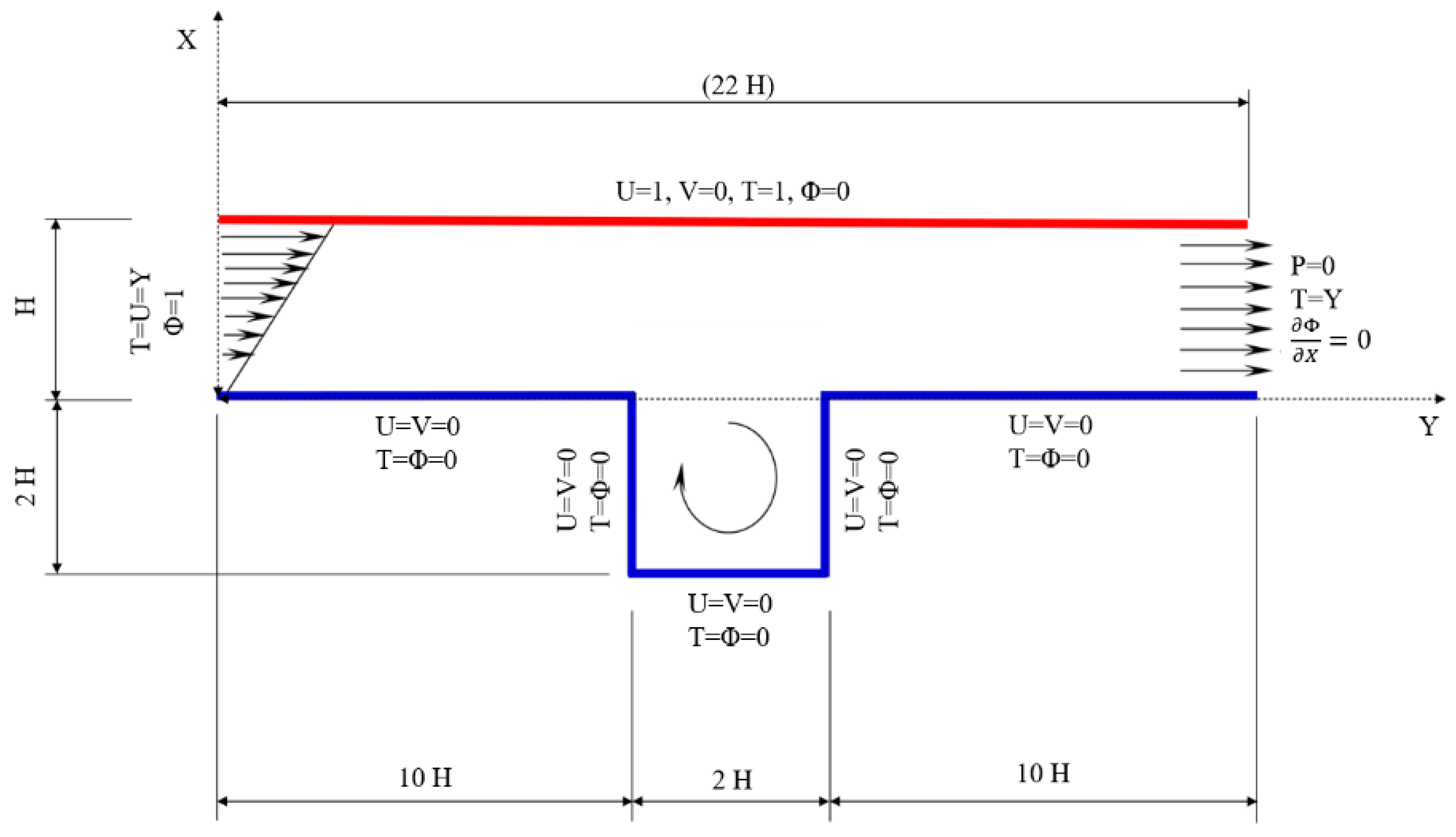
2. Mathematical Model
Let us refer to the geometry sketched in Figure 1, that is, a channel with an embedded open cavity. The characteristic lengths of the geometry under consideration are evidenced in the figure (the geometry was built according to the size of the inlet channel H).
Figure 1.
Domain and boundary conditions.
In accordance with Buongiorno’s model [11], let us consider the nanofluid as a two-component mixture (base fluid plus nanoparticles) with the flowing assumption: (i) incompressible flow, (ii) no chemical reactions, (iii) negligible external forces, (iv) dilute the mixture, (v) negligible viscous dissipation, (vi) negligible radiative heat transfer, (vii) nanoparticles and base fluid locally in thermal equilibrium. Definitely, in accordance also with Hussain and Ahmed [18], the transport model for the nanofluid is described by the following system of equations:
- Continuity equation
- Momentum equations in X and Y direction
- Energy equation
- Nanoparticles equation
In Equations (1)–(5), (U, V) are the X and Y-component of the nanofluid velocity vector, P is the nanofluid pressure, T is the nanofluid temperature, is the nanoparticles concentration. These dependent variables are given as a function of the position vector (X, Y). Furthermore, ρ is the nanofluid density, µ is the dynamic viscosity, Tc is the cold temperature, α = k/(ρ Cp) is the thermal diffusivity (k is the thermal conductivity of the fluid and Cp is the fluid-specific heat constant), δ = (ρ Cp)p/(ρ Cp)f (p and f denotes nanoparticle and the base fluid). Let us introduce the Brownian motion coefficient DB, defined by the Einstein–Stokes equation, and the thermophoresis coefficient DT, that is:
where kB is Boltzmann’s constant equal to 1.38064852 × 10⁻²³ (m2 kg)/(s2 K), dp is the nanoparticles diameter, kp is the particle thermal conductivity. For the thermal energy Equation (4), non-linearities take place with both Brownian diffusion and thermophoretic diffusion.
The boundary conditions are prescribed as follows:
- Inlet
- Outlet
- Hot wall
- Horizontal cold walls
- Vertical cold walls
In Equations (8)–(12), U0 is the slip velocity of the hot wall and Th is the temperature of the hot wall.
In detail, we investigate Couette flow: thus the boundary condition on the velocity field is the tangential motion of the upper surface with respect to the lower boundary. The effect of buoyancy is neglected. Moreover, the boundary conditions on the temperature foresee a uniform hot temperature Th on the upper wall, a uniform cold temperature Tc on the lower wall and on the cavity walls, and a linearly varying temperature distribution both at the inlet and at the outlet sections. The hot and cold walls are marked with a red and blue line, respectively, in Figure 1.
On account of the dimensionless quantities
the system of Equations (1)–(5) and Equations (8)–(12) can be rewritten in the dimensionless form as follows:
The dimensionless boundary conditions for the velocity, temperature, and concentration fields are reported in Figure 1. In Equations (14)–(23) the following dimensionless groups have been used:
where ΔT = Th − Tc.
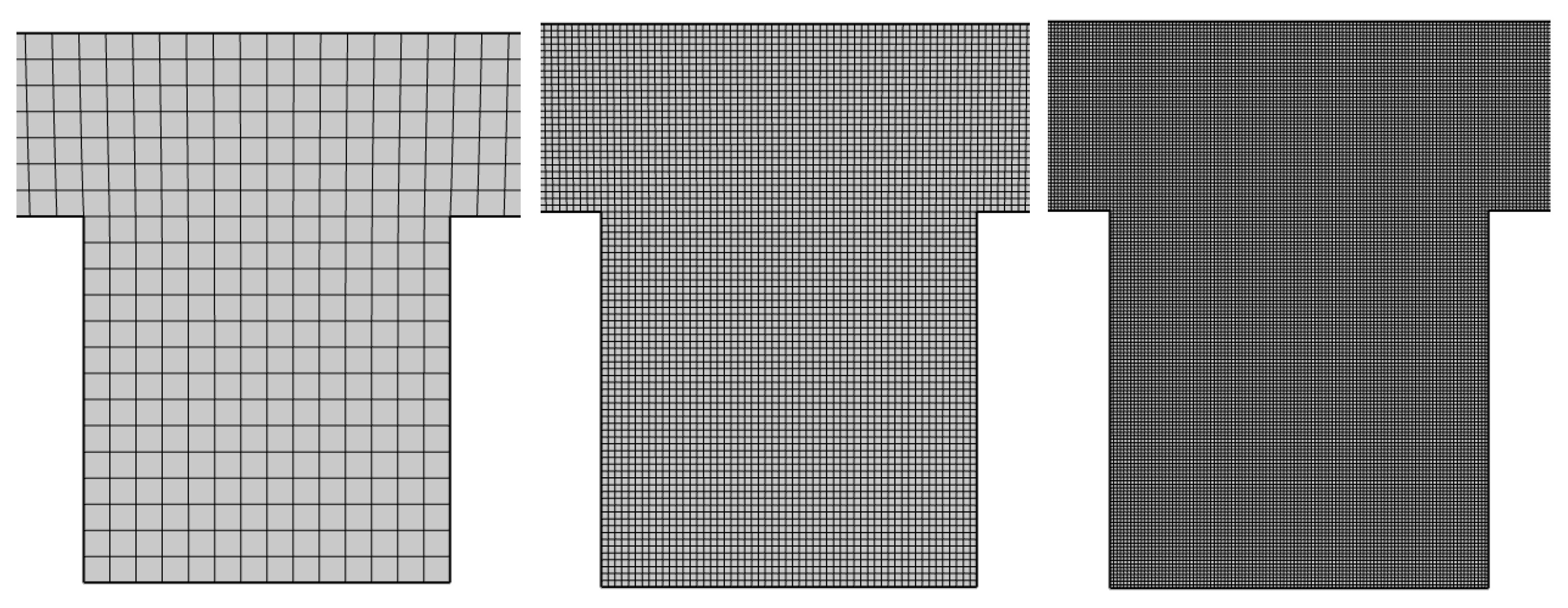
3. Mesh and Validation
First, let us introduce, for a fixed geometry configuration (Figure 1), a sensitivity analysis of the model described through Equations (14)–(23). The constants range values used for investigating the thermophoresis and Brownian diffusion are: Pr = 6.2, 50 ≤ Re ≤ 500, 0.1 ≤ Le ≤ 5, 0.1 ≤ NB ≤ 1, and 0.1 ≤ NT ≤ 1.
The mesh used for the domain discretization is made up of quadrilateral elements. In Figure 2 some of the considered meshes are shown. In particular, in order to identify the optimal number of computational elements, the following quantities are evaluated as average in the domain of interest: velocity, temperature, particle concentration, and Nusselt number on the hot wall.
Figure 2.
Mesh from coarse to fine: (left) 1246 elements, (center) 30,449 elements, (right) 59,520 elements.
For the sake of clarity, the mean volume—related to a unit depth—quantities were evaluated according to the expression
where ξ is the general non-dimensional quantities and is the non-dimensional volume under consideration. Otherwise, the mean Nusselt number is evaluated along the hot wall by the expression
where l = l1 + l2 + l3 is the total length of the hot wall.
In Table 1 the grid independence tests are reported. In the following, grid #3 will be employed.
Table 1.
Grid independence test. N is the mesh elements number, is the mean velocity, is the mean temperature, is the mean concentration and is the mean Nusselt number. The mesh validation is done for Re = 100, Pr = 6.2, NB = NT = 0.1 and Le = 10.
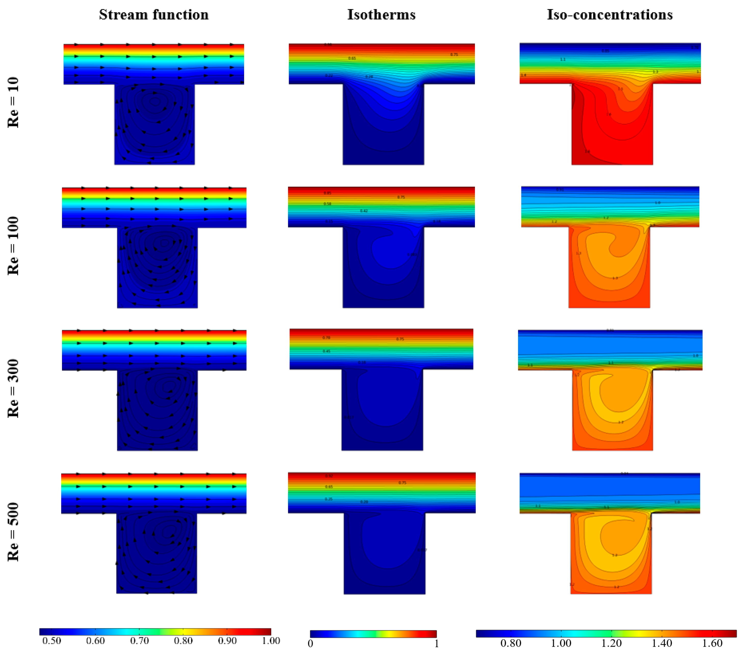
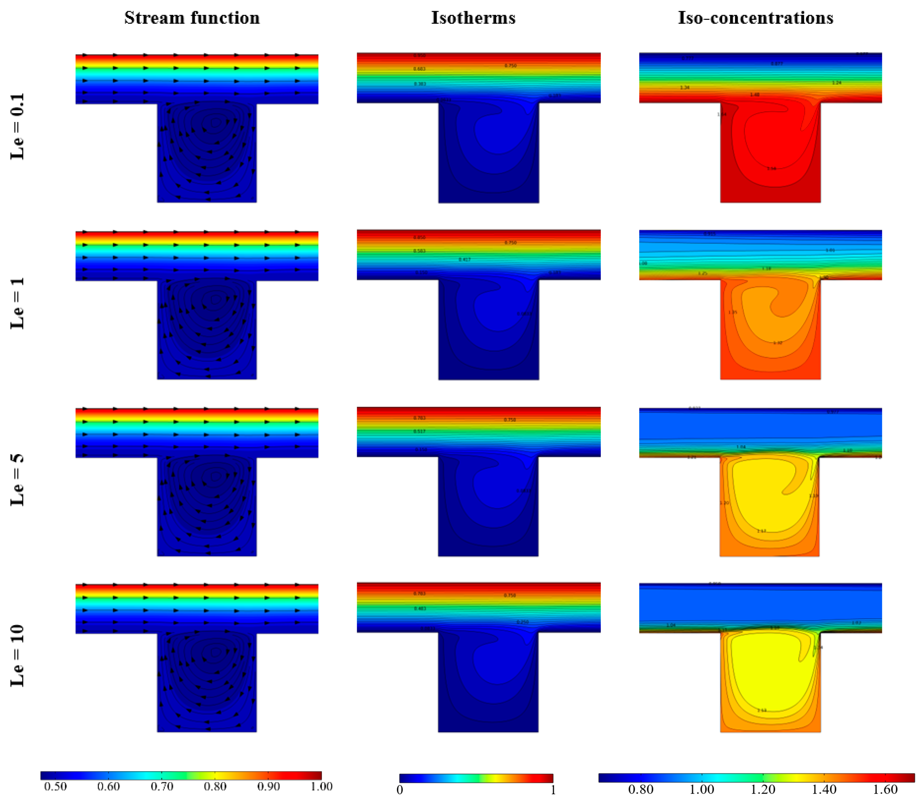
4. Results and Discussion
Let us now discuss the main features of the solutions of Equations (14)–(23). In Figure 3, Figure 4, Figure 5 and Figure 6, the velocity field stream function, the isotherms, and iso-concentration lines are reported for Pr = 6.2 and by considering the variation of one parameter (Re, Le, NB, or NT) while the other ones, respectively, are (100, 0, 0.1, 0.1).
Figure 3.
Stream function, Isotherms and Iso-concentration for various Reynolds number and Pr = 6.2, Le = 1, NB = NT = 0.1.
Figure 4.
Stream function, Isotherms and Iso-concentration for various Lewis number and Pr = 6.2, Re = 100, NB = NT = 0.1.
Figure 5.
Stream function, Isotherms and Iso-concentration for various NB number and Pr = 6.2, Re = 100, Le = 1, NT = 0.1.
Figure 6.
Stream function, Isotherms and Iso-concentration for various NT number and Pr = 6.2, Re = 100, Le = 1, NB = 0.1.
Figure 3 refers to different values assumed by the Reynolds number and shows that this parameter does not seem to affect sensibly the solution. Moreover, the figure shows that for increasing values of Re the stream function and isotherm gradients occur only in the channel region, not involving the open cavity, while the concentration gradients appear mainly in the cavity region.
Figure 4 refers to different values of the Lewis number and shows that for increasing values of Le the concentration vortex tends to occupy the whole cavity. Also, with reference to the channel region, for increasing values of the Lewis number, the concentration gradients tend to move close to the channel walls.
Figure 5 refers to different values of the Brownian diffusivity coefficient, showing that the solution is not strongly affected by this parameter: in fact, slight differences appear not only in the stream function distribution but also in the temperature and in the concentration distribution. Finally, Figure 6 refers to different values of the thermophoretic diffusivity coefficient NT, showing that also this parameter does not strongly affect the obtained solution.
In Figure 7, the dimensionless concentration (lefthand frame) and the dimensionless temperature (righthand frame) are reported versus the y- coordinate at x = (l1 + l2/2)/l, and for Pr = 6.2, Le = 1, NB = NT = 0.1 and for different values assumed by the Reynolds number. The considered X-coordinate represents the vertical middle section of the cavity. The figure shows that while for Re = 10 the functions are monotonic, for higher values local minimum and maximum arise. Moreover, the concentration assumes value 1 for any considered Re at y = 0.75. This happens because the velocity value at that point is the same for all the conditions considered. Within the cavity, strong variations of the concentration occur. The dimensionless temperature distribution varies with the vertical coordinate only in the bottom cavity region, and for every mall value of the Reynolds number is a monotonic function.
Figure 7.
Concentration and temperature for different Re number and Pr = 6.2, Le = 1, NB = NT = 0.1.
In Figure 8, the y-velocity is reported versus y at the vertical middle section of the cavity, for Pr = 6.2, Le = 1, NB = NT = 0.1, and for different values assumed by the parameter Re. The figure shows that the formation of a clockwise rotating cell in the cavity occurs and that this cell occupies a bigger region of the cavity for increasing values of Re. Moreover, the maximum of the dimensionless velocity increases for increasing values of Re.
Figure 8.
Y-velocity for different Re number and Pr = 6.2, Le = 1, NB = NT = 0.1.
In Figure 9 the dimensionless concentration and temperature distribution are reported as a function of the Lewis number. The righthand frame of the figure shows that the dimensionless temperature does not significantly vary: in fact, very small variations occur and are visible in the evidenced region, where the dimensionless temperature is an increasing function of Le. Moreover, a local maximum in the region close to the center of the cavity arises. On the contrary, the concentration strongly depends on the value assumed by the Lewis number. As discussed concerning Figure 7, the boundary condition imposes a concentration equal to 1 for any Le at the upper corner of the cavity.
Figure 9.
Concentration and temperature for different Le number and Pr = 6.2, Re = 100, NB = NT = 0.1.
In Figure 10, the dependence of the concentration and temperature fields on the Brownian diffusivity coefficient NB are reported, showing that smaller values of NB yield higher concentrations and to less uniform behavior of this function. On the contrary, NB does not affect the trend of the dimensionless temperature.
Figure 10.
Concentration and temperature for different NB number and Pr = 6.2, Re = 100, Le = 1, NT = 0.1.
Similar considerations can be done with respect to the parameter NT, as shown in Figure 11.
Figure 11.
Concentration and temperature for different NT number and Pr = 6.2, Re = 100, Le = 1, NB = 0.1.
Finally, in Figure 12 and Figure 13 the averaged Nusselt number on the hot wall is reported versus Re. Figure 12 analyzes the behavior with respect to the Brownian diffusivity coefficient (left) and to the thermophoretic diffusivity coefficient (right) and Figure 13 to the Lewis number. Figure 12 shows that the parameter NB does not affect the behavior of the Nusselt number, while NT and Le do, as evident in the right frame of Figure 12 and in Figure 13. In particular, the average Nusselt number is a decreasing function on NT, while it is an increasing function of Le. It is interesting to notice that for high values of NT, that is, NT = 0.5, the function is not monotonic, thus displaying a minimum for Re = 100.
Figure 12.
Average Nusselt number as a function of Re number for different NB number and Pr = 6.2, Le = 1, NT = 0.1 (left); Average Nusselt number as a function of Re number for different NT number and Pr = 6.2, Le = 1, NB = 0.1 (right).
Figure 13.
Average Nusselt number as a function of Re number for different Le number and Pr = 6.2, Le = 1, NB = NT = 0.1.
5. Conclusions
In the present paper, the forced convection of a nanofluid in a channel with an embedded cavity is numerically investigated. Couette flow is considered and the Buongiorno’s two-phase mixture model is employed for the description of the nanofluid. The dimensionless velocity, temperature, and concentrations field are solved by employing the software package Comsol Multiphysics, as a function of the parameters Re, Pr, Le, NB, and NT and discussed. In particular, for increasing values of Re, the stream function and isotherm gradients occur only in the channel region, not involving the open cavity, while the concentration gradients appear mainly in the cavity region. For increasing values of the Lewis number, the concentration vortex tends to occupy the whole cavity. Moreover, with reference to the channel region, for increasing values of Le the concentration gradients tend to move close to the channel walls.
Concerning the nanofluid typical effects, the thermophoretic diffusion seems to affect the solution much more than the Brownian diffusion. Finally, the average Nusselt number on the hot wall is calculated as a function of the dimensionless parameters and discussed, showing that the Brownian diffusion effects are negligible.
Author Contributions
Conceptualization, E.R.d.S.; software, A.N.I. and A.M.; validation, all authors; formal analysis, investigation, writing—original draft preparation, writing—review and editing, all authors; supervision, E.R.d.S. and C.B. All authors have read and agreed to the published version of the manuscript.
Funding
The authors wish to thank the Italian Ministry for University.
Institutional Review Board Statement
Not applicable.
Informed Consent Statement
Not applicable.
Data Availability Statement
Not applicable.
Acknowledgments
All authors agree to the recognition of the work done.
Conflicts of Interest
The authors declare no conflict of interest.
Nomenclature
| Cp | Fluid specific heat constant [J/kg K] |
| DB | Brownian motion coefficient |
| DT | Thermophoresis coefficient |
| dP | Nanoparticles diameter |
| H | Cavity dimension |
| k | Thermal conductivity [W/m K] |
| kP | Nanoparticles thermal conductivity [W/m K] |
| Le | Lewis number |
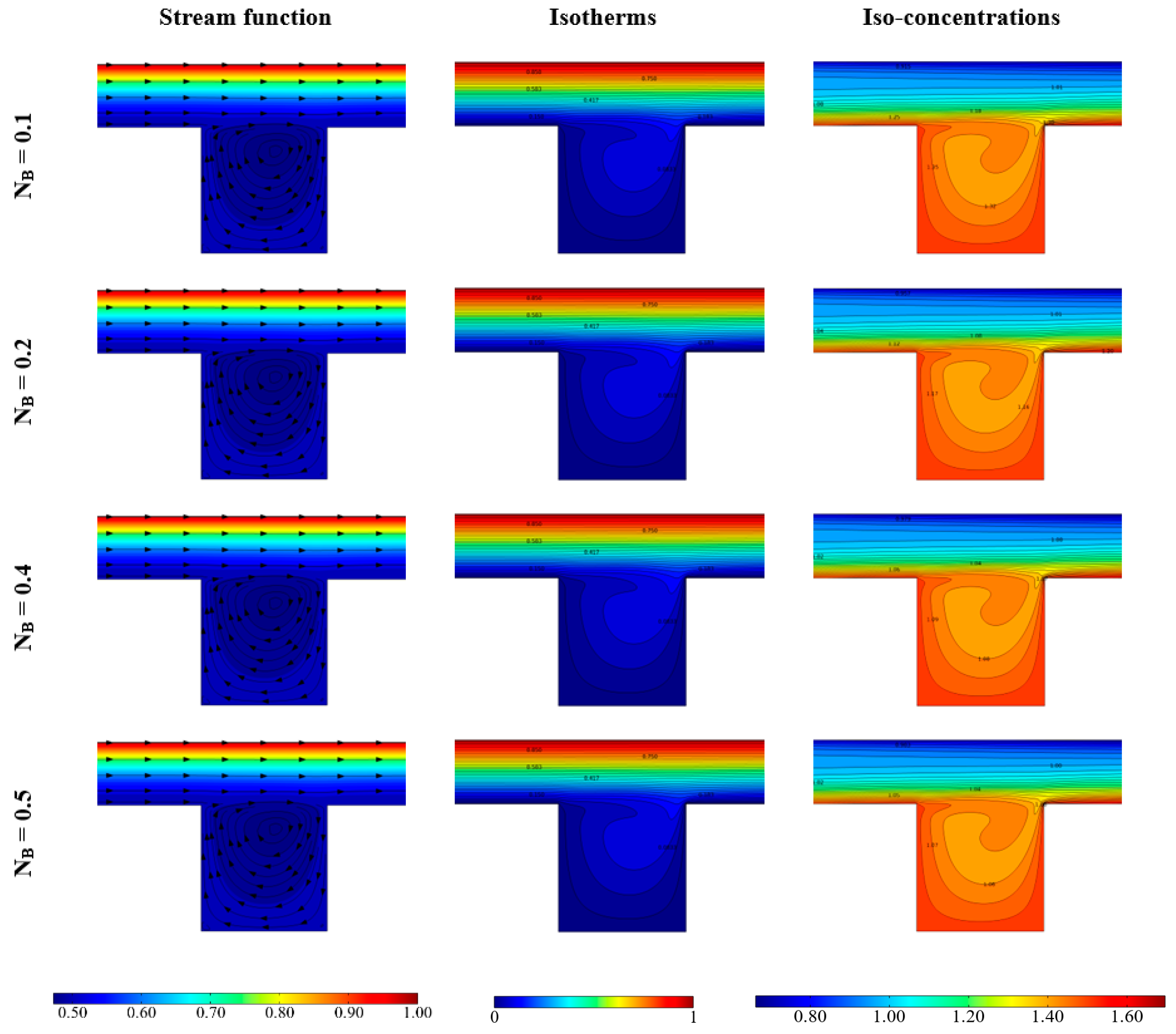
| NB | Brownian diffusivity number |
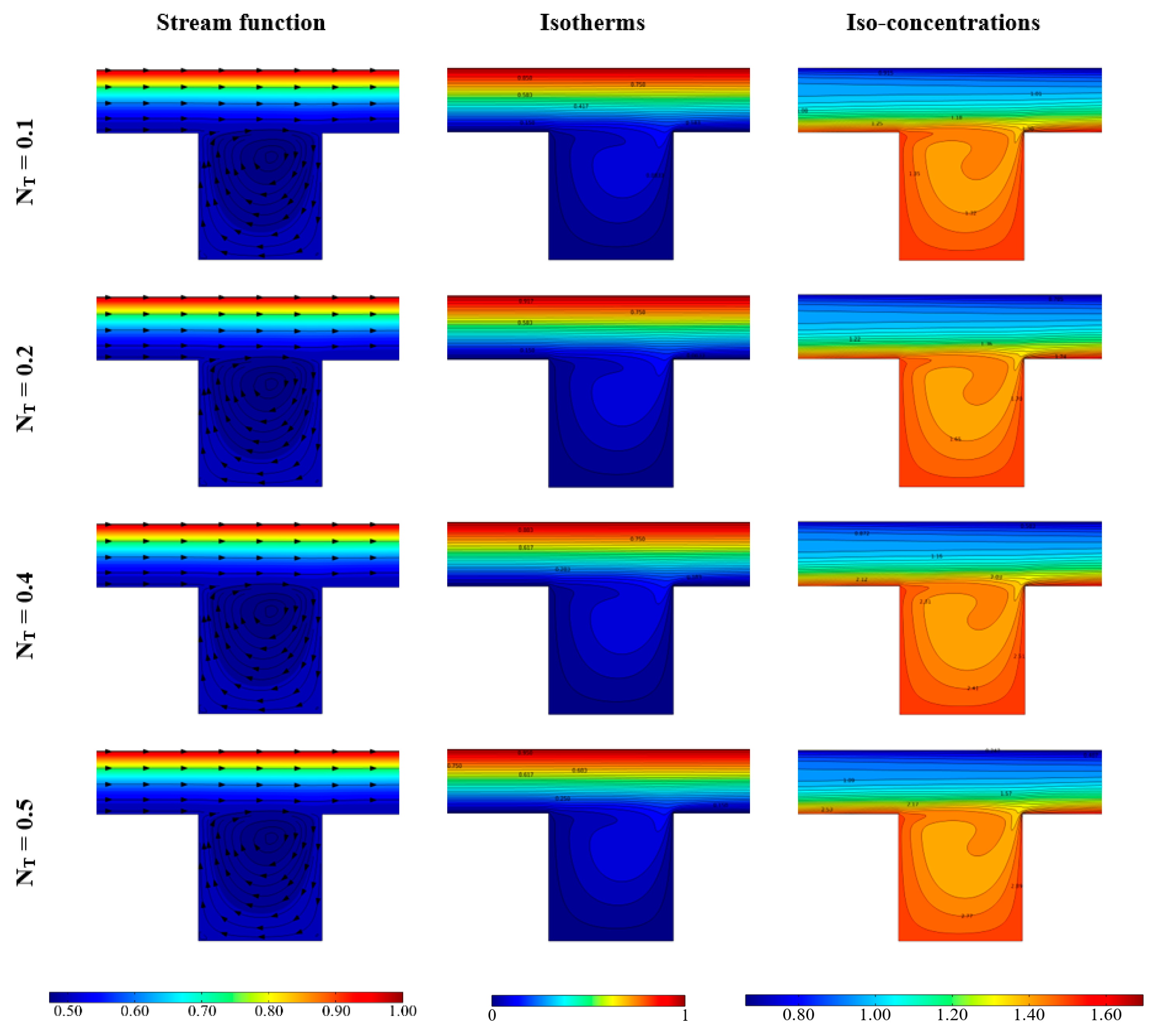
| NT | Thermophoresis number |
| Nu | Nusselt number |
| P | Nanofluid pressure [Pa] |
| p | Dimensionless pressure |
| Pr | Prandtl number |
| Re | Reynolds number |
| T | Local nanofluid temperature [K] |
| Th | Hot wall temperature [K] |
| U | x-component velocity [m/s] |
| U0 | Slip velocity [m/s] |
| V | y-component velocity [m/s] |
| (u,v) | Dimensionless velocity components |
| X | x-coordinate [m] |
| Y | y-coordinate [m] |
| (x,y) | Dimensionless coordinates |
| α | Thermal diffusivity [m2/s] |
| Θ | Dimensionless temperature |
| µ | Nanofluid dynamic viscosity [Pa s] |
| ρ | Nanofluid density [kg/m3] |
| φ | Nanoparticles concentration [#/L] |
| Φ | Dimensionless concentration |
References
- Choi, S.U.S.; Eastman, J.A. Enhancing Thermal Conductivity of Fluids with Nanoparticles: Technical Report ANL/MSD/CP-84938; CONF-951135-29; Argonne National Lab.: Lemont, IL, USA, 1995. [Google Scholar]
- Choi, S. Enhancing thermal conductivit of fluids with nanoparticles. In Developments and Applications of Non-Newtonian Flows; Siginer, D.A., Wang, H.P., Eds.; FED-V.231/MD-V; ASME: New York, NY, USA, 1995; Volume 66, pp. 99–105. [Google Scholar]
- Panduro, E.A.C.; Finotti, F.; Largiller, G.; Lervåg, K.Y. A review of the use of nanofluids as heat-transfer fluids in parabolic-trough collectors. Appl. Therm. Eng. 2022, 211, 118346. [Google Scholar] [CrossRef]
- Yan, S.R.; Aghakhani, S.; Karimipour, A. Influence of a membrane on nanofluid heat transfer and irreversibilities inside a cavity with two constant-temperature semicircular sources on the lower wall: Applicable to solar collectors. Phys. Scr. 2020, 95, 085702. [Google Scholar] [CrossRef]
- Sheremet, M.A.; Pop, I.; Mahian, O. Natural convection in an inclined cavity with time-periodic temperature boundary conditions using nanofluids: Application in solar collectors. Int. J. Heat Mass Transf. 2018, 116, 751–761. [Google Scholar] [CrossRef]
- Hady, F.M.; Ibrahim, F.S.; Abdel-Gaied, S.M.; Eid, M.R. Effect of heat generation/absorption on natural convective boundary-layer flow from a vertical cone embedded in a porous medium filled with a non-Newtonian nanofluid. Int. Commun. Heat Mass Transf. 2011, 38, 1414–1420. [Google Scholar] [CrossRef]
- Alsaedi, A.; Awais, M.; Hayat, T. Effects of heat generation/absorption on stagnation point flow of nanofluid over a surface with convective boundary conditions. Commun. Nonlinear Sci. Numer. Simul. 2012, 17, 4210–4223. [Google Scholar] [CrossRef]
- Jalilpour, B.; Jafarmadar, S.; Ganji, D.D.; Shotorban, A.B.; Taghavifar, H. Heat generation/absorption on MHD stagnation flow of nanofluid towards a porous stretching sheet with prescribed surface heat flux. J. Mol. Liq. 2014, 195, 194–204. [Google Scholar] [CrossRef]
- Rawat, S.K.; Mishra, A.; Kumar, M. Numerical study of thermal radiation and suction effects on copper and silver water nanofluids past a vertical Riga plate. Multidiscip. Model. Mater. Struct. 2019, 15, 714–736. [Google Scholar] [CrossRef]
- Patil, P.M.; Shashikant, A.; Hiremath, P.S. Diffusion of liquid hydrogen and oxygen in nonlinear mixed convection nanofluid flow over vertical cone. Int. J. Hydrog. Energy 2019, 44, 17061–17071. [Google Scholar] [CrossRef]
- Buongiorno, J. Convective transport in nanofluids. J. Heat Transf. 2006, 128, 240–250. [Google Scholar] [CrossRef]
- Azimikivi, H.; Purmahmud, N.; Mirzaee, I. Rib shape and nanoparticle diameter effects on natural convection heat transfer at low turbulence two-phase flow of AL2O3-water nanofluid inside a square cavity: Based on Buongiorno’s two-phase model. Therm. Sci. Eng. Prog. 2020, 20, 100587. [Google Scholar] [CrossRef]
- Rawat, S.K.; Upreti, H.; Kumar, M. Comparative Study of Mixed Convective MHD Cu-Water Nanofluid Flow over a Cone and Wedge using Modified Buongiorno’s Model in Presence of Thermal Radiation and Chemical Reaction via Cattaneo-Christov Double Diffusion Model. J. Appl. Comput. Mech. 2021, 7, 1383–1402. [Google Scholar]
- Ma, Y.; Mohebbi, R.; Rashid, M.M.; Yang, Z. Study of nanofluid forced convection heat transfer in a bent channel by means of lattice Boltzmann method. Phys. Fluids 2018, 30, 032001. [Google Scholar] [CrossRef]
- Rossi di Schio, E.; Celli, M.; Barletta, A. Effects of Brownian Diffusion and Thermophoresis on the Laminar Forced Convection of a Nanofluid in a Channel. J. Heat Transf. 2014, 136, 022401. [Google Scholar] [CrossRef]
- Mehrez, Z.; Bouterra, M.; El Cafsi, A.; Belghith, A. Heat transfer and entropy generation analysis of nanofluids flow in an open cavity. Comput. Fluids 2013, 88, 363–373. [Google Scholar] [CrossRef]
- Makinde, O.D.; Omar, A.; Tshehla, M.S. Computational Modelling of Couette Flow of Nanofluids with Viscous Heating and Convective Cooling. J. Comput. Math. 2014, 2014, 631749. [Google Scholar] [CrossRef] [Green Version]
- Ellahi, R.; Sait, S.M.; Shehzad, N.; Mobin, N. Numerical Simulation and Mathematical Modeling of Electro-Osmotic Couette–Poiseuille Flow of MHD Power-Law Nanofluid with Entropy Generation. Symmetry 2019, 11, 1038. [Google Scholar] [CrossRef] [Green Version]
- Hussain, S.; Sameh, E.A.; Akbar, T. Entropy generation analysis in MHD mixed convection of hybrid nanofluid in an open cavity with a horizontal channel containing an adiabatic obstacle. Int. J. Heat Mass Transf. 2017, 114, 1054–1066. [Google Scholar] [CrossRef]
- Seyyedi, S.M.; Dogonchi, A.S.; Hashemi-Tilehnoee, M.; Waqas, M.; Ganji, D.D. Entropy generation and economic analyses in a nanofluid filled L-shaped enclosure subjected to an oriented magnetic field. Appl. Therm. Eng. 2020, 168, 114789. [Google Scholar] [CrossRef]
- Biserni, C.; Impiombato, A.N.; Aminhossein, J.; Rossi di Schio, E.; Semprini, G. Formation and Topology of vortices in Couette Flow over open cavities. In E3S Web of Conferences; EDP Sciences: Les Ulis, France, 2020; Volume 197, p. 10005. [Google Scholar]
Publisher’s Note: MDPI stays neutral with regard to jurisdictional claims in published maps and institutional affiliations. |
© 2022 by the authors. Licensee MDPI, Basel, Switzerland. This article is an open access article distributed under the terms and conditions of the Creative Commons Attribution (CC BY) license (https://creativecommons.org/licenses/by/4.0/).