
Improving Path Loss Prediction Using Environmental Feature Extraction from Satellite Images: Hand-Crafted vs. Convolutional Neural Network


Abstract
:1. Introduction
- Review of path loss prediction based on image processing using CNN.Most works presented ML-based image processing approaches for path loss prediction, but to the best of our knowledge, no such comprehensive review of such existing works was supplied.
- Investigation on the use of various hand-crafted feature extraction techniques and their combinations on 2D satellite images in path loss prediction.
- Combining CNN features with hand-crafted features to improve the accuracy of path loss prediction.While this has been applied in computer vision tasks, to the best of our knowledge, this has not been applied to the problem of path loss prediction.
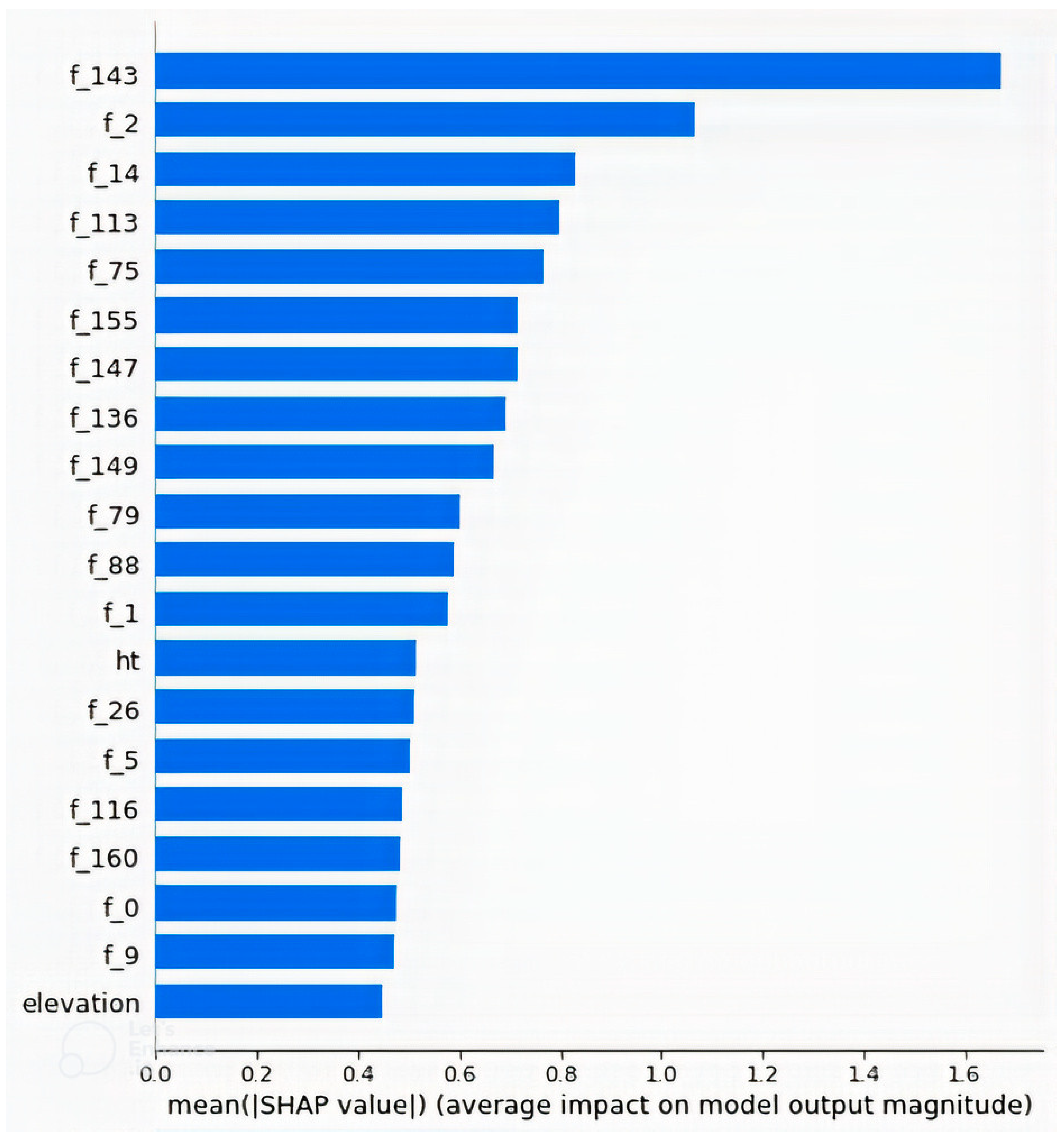
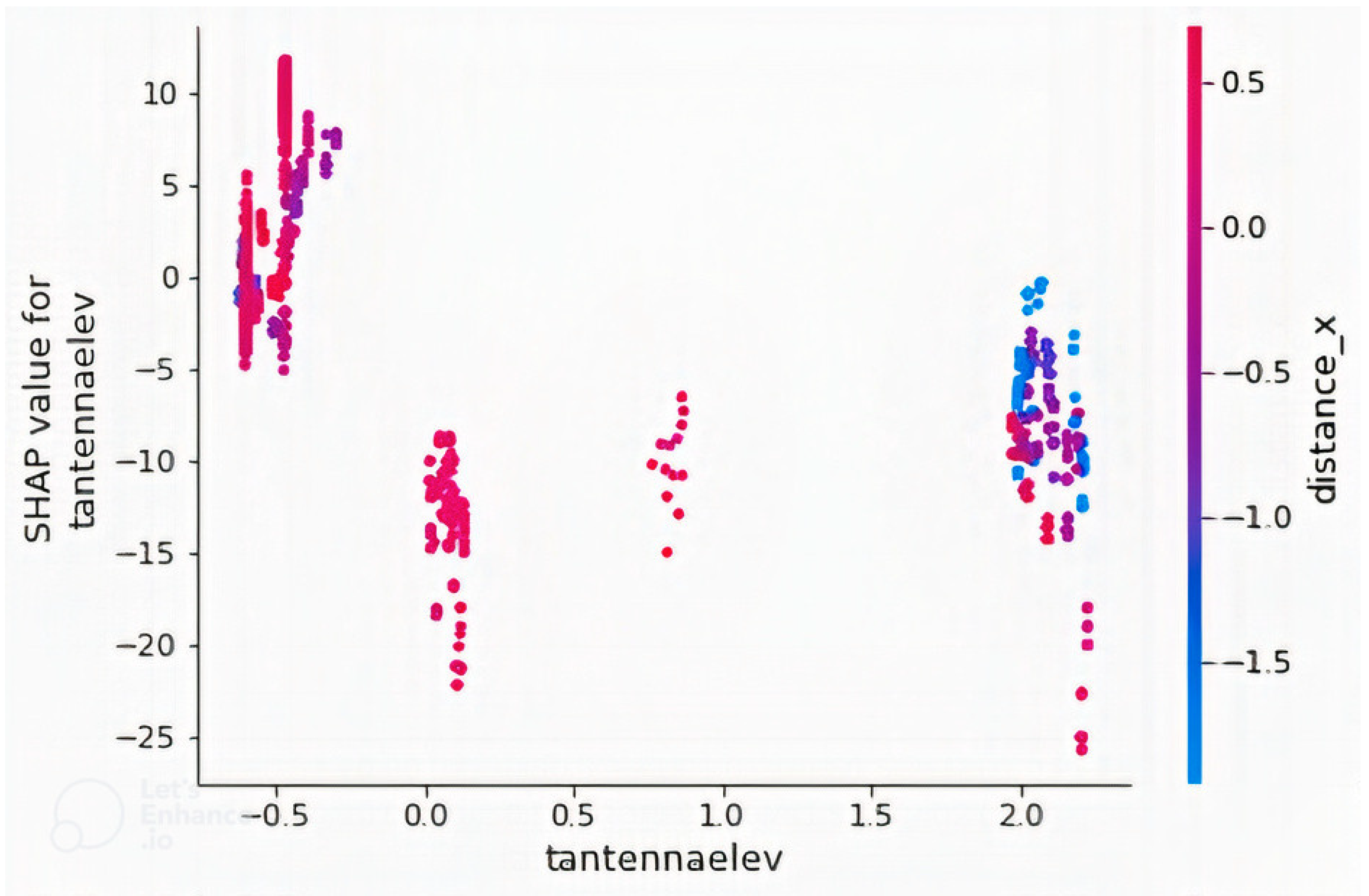
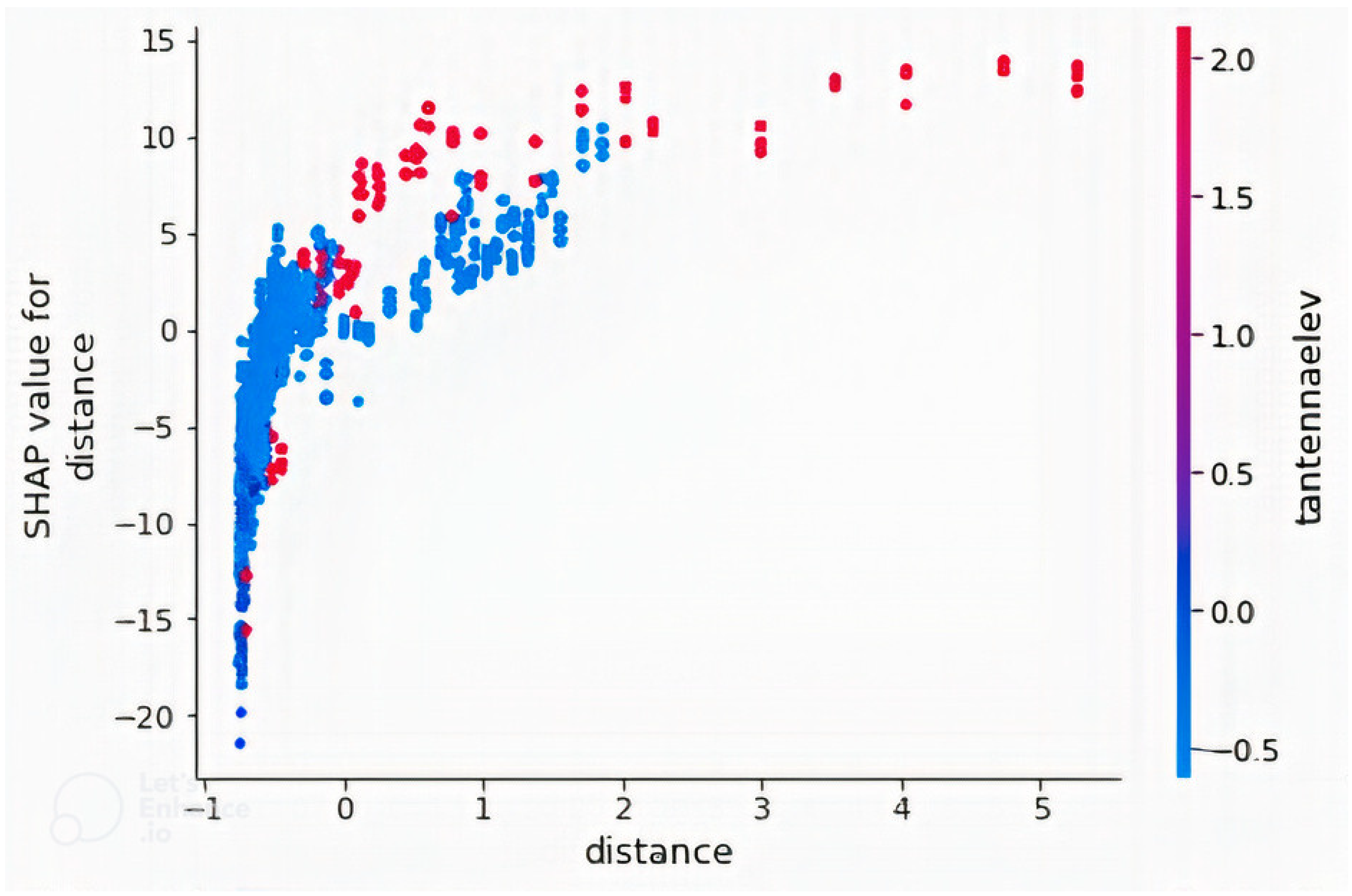
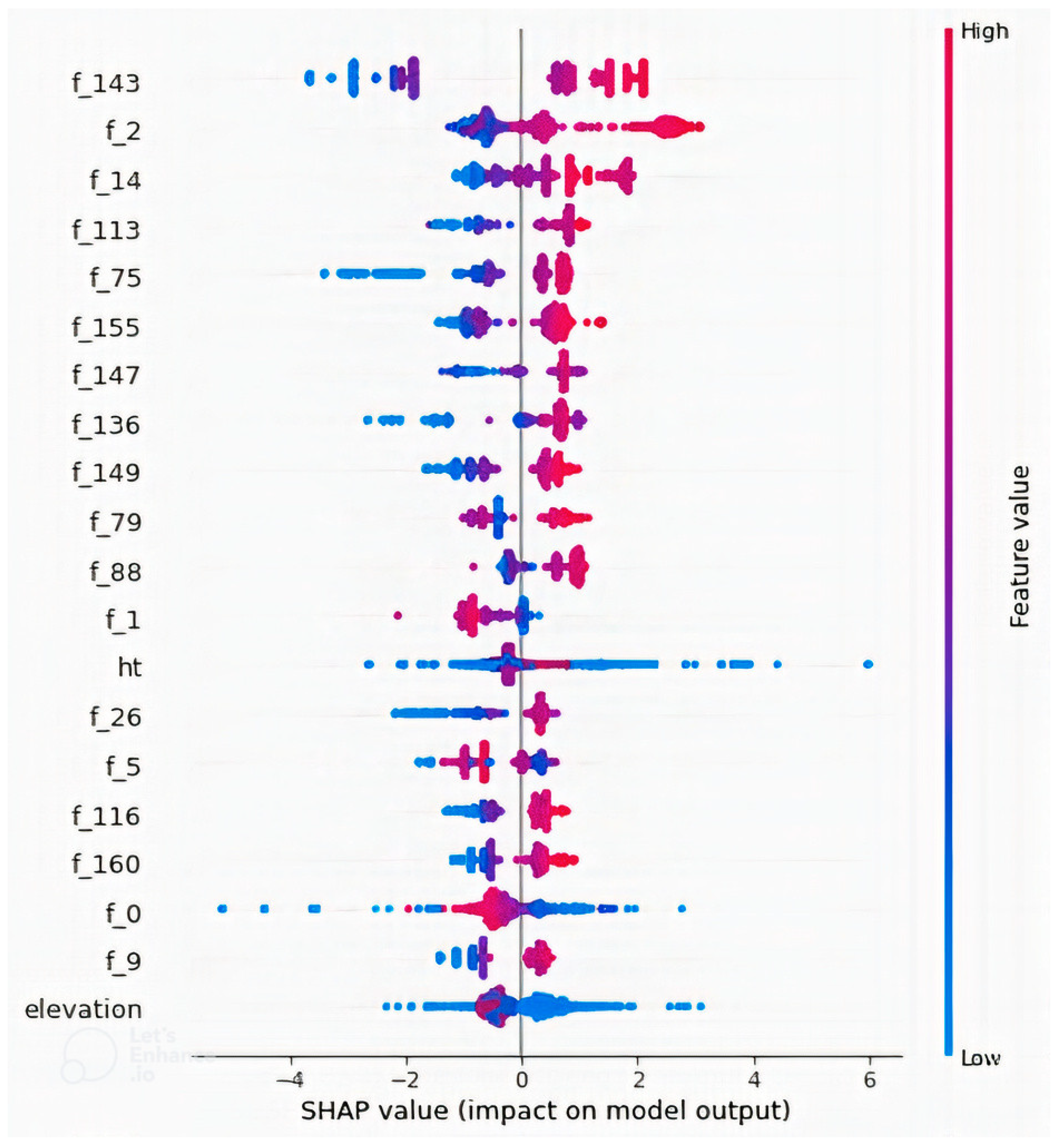
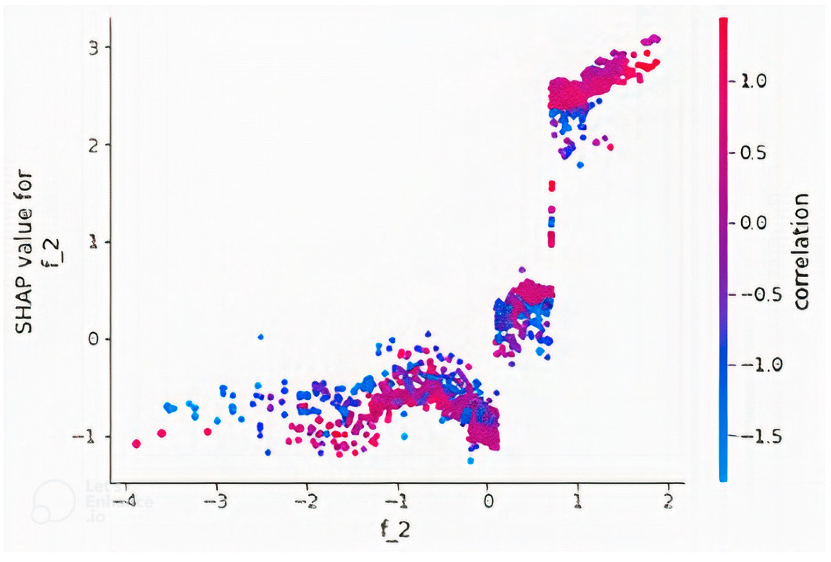
- Interpretation of model prediction based on Shapley Additive Explanations (SHAP).Most ML-based path loss prediction works do not analyze the features deeply, including the comparison of different types of features.
2. Related Works
2.1. Satellite Images
2.1.1. Training a Customized CNN with Satellite Images
2.1.2. Transfer Learning with Satellite Images
2.2. Segmented Images
2.2.1. Training a Customized CNN with Segmented Images
2.2.2. Training Modified UNet Architecture with Segmented Images
2.3. Combination of Images
2.4. Pseudoimages
2.5. Summary
3. Methodology
3.1. Dataset
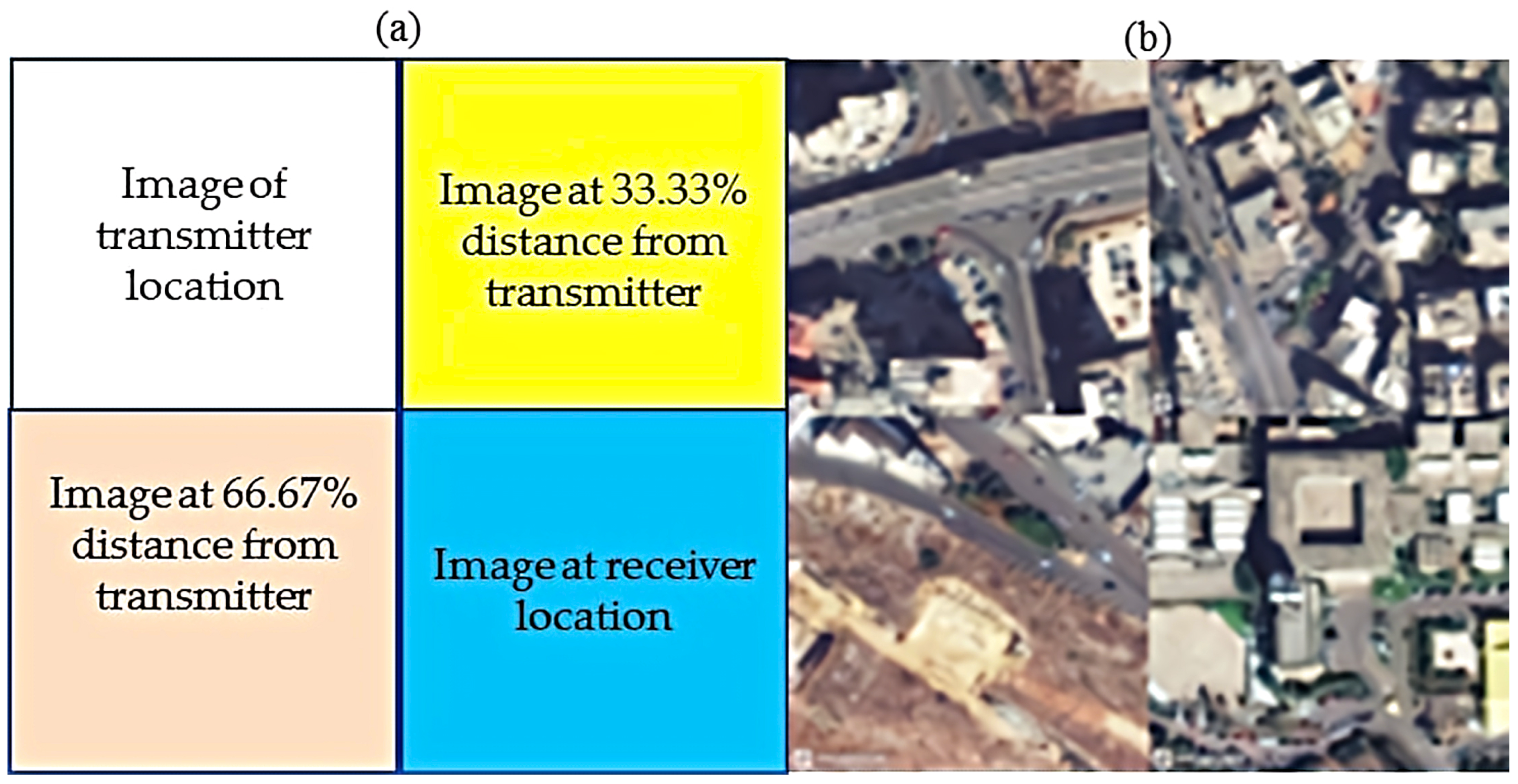
3.2. Image Data
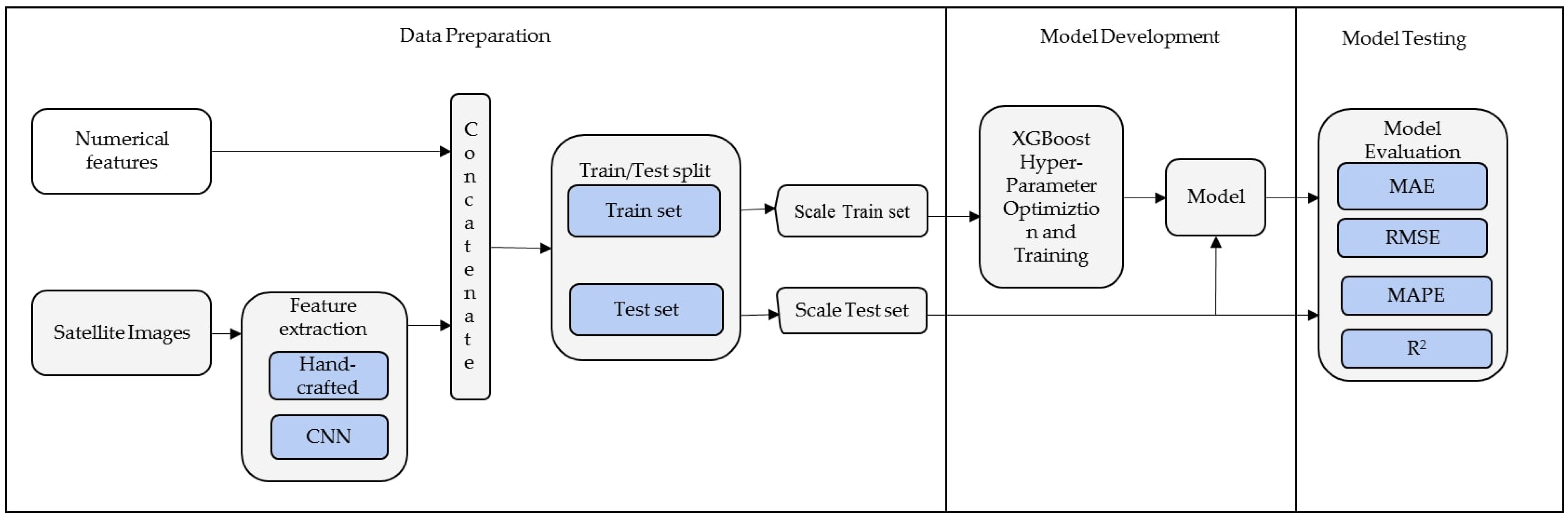
3.3. Proposed Method
3.3.1. Data Preparation
3.3.2. Model Development
3.3.3. Model Testing
3.4. Feature Extraction Methods
3.4.1. Local Binary Pattern (LBP)
3.4.2. Gray Level Co-Occurrence Matrix (GLCM)
3.4.3. Histogram of Oriented Gradients (HOG)
3.4.4. Discrete Wavelet Transform (DWT)
3.4.5. Segmentation Fractal-Based Texture Analysis (SFTA)
3.4.6. Convolutional Neural Networks (CNN)
3.5. Extreme Gradient Boosting (XGBoost)
3.6. Performance Metrics
4. Result and Discussions
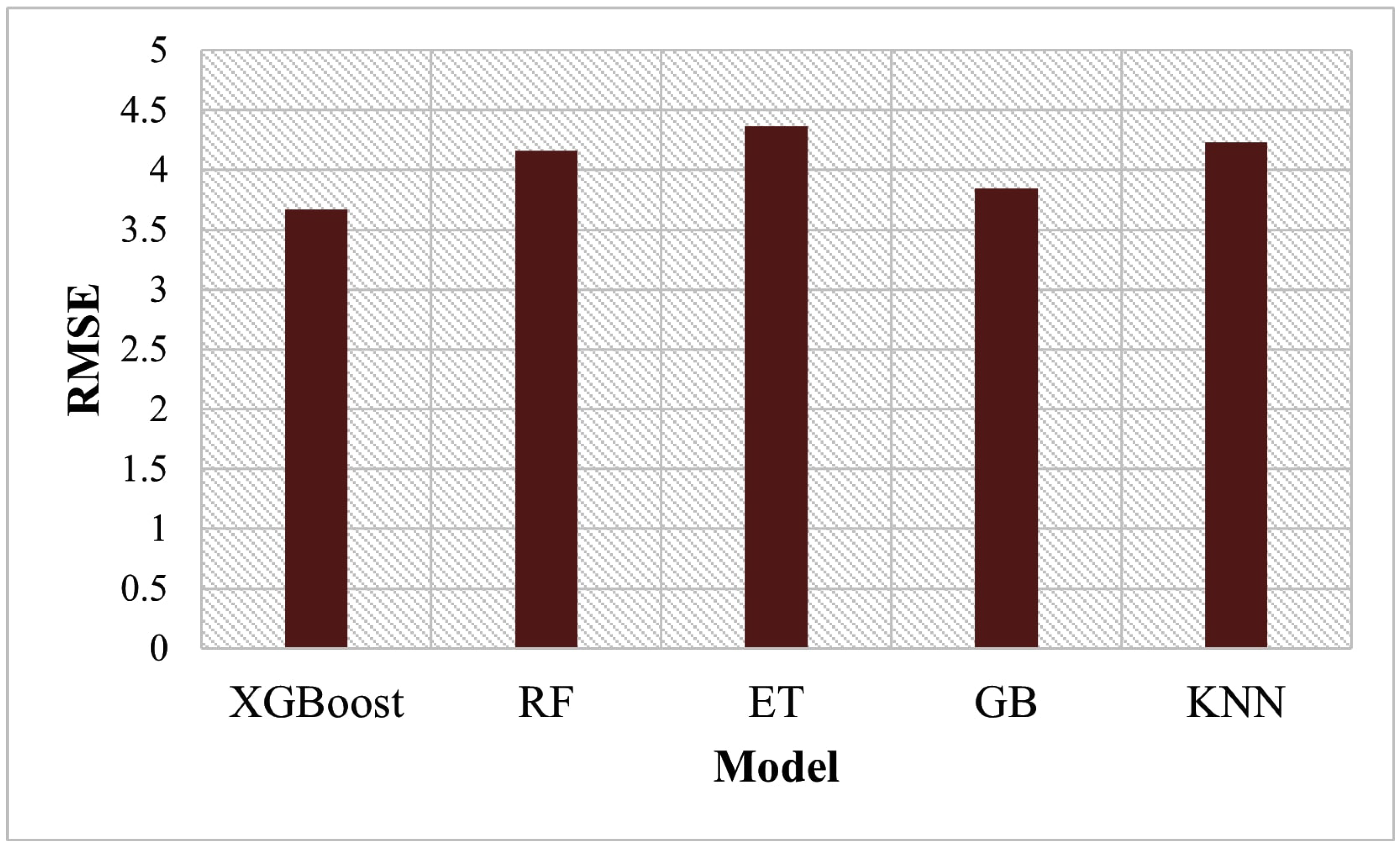
4.1. Comparison of XGBoost with Other Algorithms
4.2. Feature Importance
5. Conclusions
Author Contributions
Funding
Institutional Review Board Statement
Informed Consent Statement
Data Availability Statement
Acknowledgments
Conflicts of Interest
References
- Lukman, S.; Nazaruddin, Y.Y.; Ai, B.; He, R.; Joelianto, E. Estimation of received signal power for 5G-railway communication systems. In Proceedings of the 6th International Conference on Electric Vehicular Technology (ICEVT 2019), Bali, Indonesia, 18–21 November 2019; pp. 35–39. [Google Scholar]
- Jo, H.S.; Park, C.; Lee, E.; Choi, H.K.; Park, J. Path Loss Prediction Based on Machine Learning Techniques: Principal Component Analysis, Artificial Neural Network and Gaussian Process. Sensors 2020, 20, 1927. [Google Scholar] [CrossRef] [Green Version]
- Zhang, Y.; Wen, J.; Yang, G.; He, Z.; Wang, J. Path Loss Prediction Based on Machine Learning: Principle, Method, and Data Expansion. Appl. Sci. 2019, 9, 1908. [Google Scholar] [CrossRef] [Green Version]
- Sotiroudis, S.P.; Goudos, S.K.; Siakavara, K.F.I.A. Tool to Explain Radio Propagation and Reduce Model Complexity. Telecom 2020, 1, 114–125. [Google Scholar] [CrossRef]
- Moraitis, N.; Tsipi, L.; Vouyioukas, D.; Gkioni, A.; Louvros, S. Performance Evaluation of Machine Learning Methods for Path Loss Prediction in Rural Environment at 3.7GHz. Wirel. Netw. 2021, 27, 4169–4188. [Google Scholar] [CrossRef]
- Isabona, J.; Imoize, A.; Ojo, S.; Karunwi, O.; Kim, Y.; Lee, C.; Li, C. Development of a Multilayer Perceptron Neural Network for Optimal Predictive Modeling in Urban Microcellular Radio Environments. Appl. Sci. 2022, 12, 5713. [Google Scholar] [CrossRef]
- Ahmadien, O.; Ates, H.F.; Baykas, T.; Gunturk, B.K. Predicting Path Loss Distribution of an Area from Satellite Images Using Deep Learning. IEEE Access 2020, 8, 64982–64991. [Google Scholar] [CrossRef]
- Thrane, J.; Zibar, D.; Christiansen, H.L. Model-Aided Deep Learning Method for Path Loss Prediction in Mobile Communication Systems at 2.6 GHz. IEEE Access 2020, 8, 7925–7936. [Google Scholar] [CrossRef]
- Sotiroudis, S.P.; Goudos, S.K.; Siakavara, K. Deep Learning for Radio Propagation: Using Image-Driven Regression to Estimate Path Loss in Urban Areas. ICT Express 2020, 6, 160–165. [Google Scholar] [CrossRef]
- Lee, J.G.Y.; Kang, M.Y.; Kim, S.C. Path loss exponent prediction for outdoor millimeter wave channels through deep learning. In Proceedings of the IEEE Conference on Wireless Communications and Networking, Marrakech, Morocco, 15–18 April 2019. [Google Scholar]
- Sotiroudis, S.P.; Sarigiannidis, P.; Goudos, S.K.; Siakavara, K. Fusing Diverse Input Modalities for Path Loss Prediction: A Deep Learning Approach. IEEE Access 2021, 9, 30441–30451. [Google Scholar] [CrossRef]
- Omoze, E.L.; Edeko, F.O. Statistical Tuning of COST 231 Hata Model in Deployed 1800 MHz GSM Networks for a Rural Environment. Niger. J. Technol. 2021, 39, 1216–1222. [Google Scholar] [CrossRef]
- Cahyadi, M.B.; Sudiarta, P.K.; Hartawan, D.D.; Analisis, I.G.A.K. Perbandingan Nilai Shadow Fading Pada Model Propagasi Stanford University Interim ( Sui ) Dengan Metode Simulasi Dan Drive Test. J. Spektrum 2021, 8, 230–242. [Google Scholar]
- Ayadi, M.; Zineb, B.; Tabbane, A.; Uhf, S.A. Path Loss Model Using Learning Machine for Heterogeneous Networks. IEEE Trans. Antennas Propag. 2017, 65, 3675–3683. [Google Scholar] [CrossRef]
- Nguyen, C.; Cheema, A.A. A Deep Neural Network-Based Multi-Frequency Path Loss Prediction Model from 0.8 GHz to 70 GHz. Sensors 2021, 21, 5100. [Google Scholar] [CrossRef] [PubMed]
- Sani, U.S.; Lai, D.T.C.; Malik, O.A. A hybrid combination of a convolutional neural network with a regression model for path loss prediction using tiles of 2D satellite images. In Proceedings of the 8th International Conference on Intelligent and Advanced Systems (ICIAS), Kuching, Malaysia, 13–15 July 2021. [Google Scholar]
- Sani, U.S.; Lai, D.T.C.; Malik, O.A. Investigating Automated Hyper-Parameter Optimization for a Generalized Path Loss Model. In Proceedings of the 11th International Conference on Electronics Communications and Networks (CECNet), Beijing, China, 18–21 November 2021; pp. 283–291. [Google Scholar]
- Sotiroudis, S.P.; Siakavara, K.; Koudouridis, G.P.; Sarigiannidis, P.; Goudos, S.K. Enhancing Machine Learning Models for Path Loss Prediction Using Image Texture Techniques. IEEE Antennas Wirel. Propag. Lett. 2021, 20, 1443–1447. [Google Scholar] [CrossRef]
- Bodapati, J.D.; Suvarna, B.; Veeranjaneyulu, N. Role of Deep Neural Features vs Hand Crafted Features for Hand Written Digit Recognition. Int. J. Recent Technol. Eng 2019, 7, 147–152. [Google Scholar]
- Sumi, T.A.; Hossain, M.S.; Islam, R.U.; Andersson, K. Human Gender Detection from Facial Images Using Convolution Neural Network. In Proceedings of the Communications in Computer and Information Science, Nottingham, UK, 30–31 July 2021; Volume 1435, pp. 188–203. [Google Scholar]
- Lin, W.; Hasenstab, K.; Cunha, G.M.; Schwartzman, A. Comparison of Handcrafted Features and Convolutional Neural Networks for Liver MR Image Adequacy Assessment. Sci. Rep. 2020, 10, 20336. [Google Scholar] [CrossRef] [PubMed]
- Nanni, L.; Ghidoni, S.; Brahnam, S. Handcrafted vs. Non-Handcrafted Features for Computer Vision Classification. Pattern Recognit. 2017, 71, 158–172. [Google Scholar] [CrossRef]
- Thrane, J.; Sliwa, B.; Wietfeld, C.; Christiansen, H.L. Deep learning-based signal strength prediction using geographical images and expert Knowledge. In Proceedings of the 2020 IEEE Global Communications Conference, Taipei, Taiwan, 7–11 December 2020. [Google Scholar]
- Sliwa, B.; Geis, M.; Bektas, C.; Lop, M.; Mogensen, P.; Wietfeld, C. DRaGon: Mining latent radio channel information from geographical data leveraging deep learning. In Proceedings of the 2022 IEEE Wireless Communications and Networking Conference (WCNC), Austin, TX, USA, 10–13 April 2022. [Google Scholar]
- Nguyen, T.T.; Caromi, R.; Kallas, K.; Souryal, M.R. Deep learning for path loss prediction in the 3.5 GHz CBRS spectrum band. In In Proceedings of the 2022 IEEE Wireless Communications and Networking Conference (WCNC), Austin, TX, USA, 10–13 April 2022. [Google Scholar]
- Ates, H.F.; Hashir, S.M.; Baykas, T.; Gunturk, B.K. Path Loss Exponent and Shadowing Factor Prediction From Satellite Images Using Deep Learning. IEEE Access 2019, 7, 101366–101375. [Google Scholar] [CrossRef]
- Cheng, H.; Lee, H.; Cho, M. Millimeter Wave Path Loss Modeling for 5G Communications Using Deep Learning With Dilated Convolution and Attention. IEEE Access 2021, 9, 62867–62879. [Google Scholar] [CrossRef]
- Kim, H.; Jin, W.; Lee, H. MmWave Path Loss Modeling for Urban Scenarios Based on 3D-Convolutional Neural Networks. In Proceedings of the 2022 International Conference on Information Networking (ICOIN), Jeju, Korea, 12–15 January 2022. [Google Scholar]
- Wu, L.; He, D.; Ai, B.; Wang, J.; Liu, D.; Zhu, F. Enhanced Path Loss Model by Image-Based Environmental Characterization. IEEE Antennas Wirel. Propag. Lett. 2022, 21, 903–907. [Google Scholar] [CrossRef]
- Ratnam, V.V.; Chen, H.; Pawar, S.; Zhang, B.; Zhang, C.J.; Kim, Y.J.; Lee, S.; Cho, M.; Yoon, S.R. FadeNet: Deep Learning-Based Mm-Wave Large-Scale Channel Fading Prediction and Its Applications. IEEE Access 2021, 9, 3278–3290. [Google Scholar] [CrossRef]
- Zhang, X.; Shu, X.; Zhang, B.; Ren, J.; Zhou, L.; Chen, X. Cellular network radio propagation modeling with deep convolutional neural networks. In Proceedings of the 26th ACM SIGKDD International Conference on Knowledge Discovery and Data Mining, San Diego, CA, USA, 6–10 July 2020; pp. 2378–2386. [Google Scholar]
- Hayashi, T.; Nagao, T.; Ito, S.A. A Study on the variety and size of input data for radio propagation prediction using a deep neural network. In Proceedings of the 2020 14th European Conference on Antennas and Propagation (EuCAP), Copenhagen, Denmark, 15–20 March 2020. [Google Scholar]
- Inoue, K.; Ichige, K.; Nagao, T.; Hayashi, T. Radio Propagation Prediction Using Deep Neural Network and Building Occupancy Estimation. IEICE Commun. Express 2020, 9, 506–511. [Google Scholar] [CrossRef]
- SVR PATHLOSS. Available online: https://github.com/timotrob/SVR_PATHLOSS (accessed on 2 January 2022).
- LoRaWAN Measurement Campaigns in Lebanon. Available online: https://zenodo.org/record/1560654#.X-9B-VUzbIV (accessed on 2 January 2022).
- Path Loss Prediction. Available online: https://github.com/lamvng/Path-loss-prediction (accessed on 2 January 2022).
- Timoteo, R.D.A.; Cunha, D.C.; Cavalcanti, G.D.C. A Proposal for Path Loss Prediction in Urban Environments Using Support Vector Regression. In Proceedings of the The Tenth Advanced International Conference on Telecommunications, Paris, France, 20–24 July 2014; pp. 119–124. [Google Scholar]
- El Chall, R.; Lahoud, S.; El Helou, M. LoRaWAN Network Radio Propagation Models and Performance Evaluation in Various Environments in Lebanon. IEEE Internet Things J. 2019, 6, 2366–2378. [Google Scholar] [CrossRef]
- Popoola, S.I.; Atayero, A.A.; Arausi, O.D.; Matthews, V.O. Path Loss Dataset for Modeling Radio Wave Propagation in Smart Campus Environment. Data Br. 2018, 17, 1062–1073. [Google Scholar] [CrossRef] [PubMed]
- Mapbox. Static Maps. 2022. Available online: https://www.mapbox.com/static-maps (accessed on 18 January 2022).
- Li, L.; Jamieson, K.; DeSalvo, G.; Rostamizadeh, A.; Talwalkar, A. Hyperband: A Novel Bandit-Based Approach To Hyperparameter Optimization. J. Mach Learn. Res. 2018, 18, 6765–6816. [Google Scholar]
- Horn, Z.C.; Auret, L.; McCoy, J.T.; Aldrich, C.; Herbst, B.M. Performance of Convolutional Neural Networks for Feature Extraction in Froth Flotation Sensing. IFAC-PapersOnLine 2017, 50, 13–18. [Google Scholar] [CrossRef]
- Wang, S.; Han, K.; Jin, J. Review of Image Low-Level Feature Extraction Methods for Content-Based Image Retrieval. Sens. Rev. 2019, 39, 783–809. [Google Scholar] [CrossRef]
- Paramkusham, S.; Rao, K.M.M.; Rao, B.P. Comparison of Rotation Invariant Local Frequency, LBP and SFTA Methods for Breast Abnormality Classification. Int. J. Signal Imaging Syst. Eng. 2018, 11, 136–150. [Google Scholar] [CrossRef]
- Choras, R.S. Image Feature Extraction Techniques and Their Applications for CBIR and Biometrics Systems. Int. J. Biol. Biomed. Eng. 2007, 1, 6–15. [Google Scholar]
- Sukiman, T.S.A.; Suwilo, S.; Zarlis, M. Feature Extraction Method GLCM and LVQ in Digital Image-Based Face Recognition. SinkrOn 2019, 4, 1–4. [Google Scholar] [CrossRef]
- Casagrande, L.; Macarini, L.A.B.; Bitencourt, D.; Fröhlich, A.A.; de Araujo, G.M.A. New Feature Extraction Process Based on SFTA and DWT to Enhance Classification of Ceramic Tiles Quality. Mach. Vis. Appl. 2020, 31, 71. [Google Scholar] [CrossRef]
- Althnian, A.; Aloboud, N.; Alkharashi, N.; Alduwaish, F.; Alrshoud, M.; Kurdi, H. Face Gender Recognition in the Wild: An Extensive Performance Comparison of Deep-Learned, Hand-Crafted, and Fused Features with Deep and Traditional Models. Appl. Sci. 2021, 11, 89. [Google Scholar] [CrossRef]
- Ghazali, K.H.; Mansor, M.F.; Mustafa, M.M.; Hussain, A. Feature extraction technique using discrete wavelet transform for image classification. In Proceedings of the 2007 5th Student Conference on Research and Development, Selangor, Malaysia, 11–12 December 2007. [Google Scholar]
- Costa, A.F.; Humpire-Mamani, G.; Traina, A.J.M.H. An Efficient Algorithm for Fractal Analysis of Textures. In Proceedings of the Brazilian Symposium on Computer Graphics and Image Processing, Ouro Preto, Brazil, 22–25 August 2012; pp. 39–46. [Google Scholar]
- Yamashita, R.; Nishio, M.; Do, R.K.G.; Togashi, K. Convolutional Neural Networks: An Overview and Application in Radiology. Insights Imaging 2018, 9, 611–629. [Google Scholar] [CrossRef] [Green Version]
- Ranjbar, S.; Nejad, F.M.; Zakeri, H.; Gandomi, A.H. Computational intelligence for modeling of asphalt pavement surface distress. In New Materials in Civil Engineering; Elsevier: Oxford, UK, 2020. [Google Scholar]
- Weimer, D.; Scholz-reiter, B.; Shpitalni, M. Design of Deep Convolutional Neural Network Architectures for Automated Feature Extraction in Industrial Inspection. CIRP Ann. Manuf. Technol. 2016, 65, 417–420. [Google Scholar] [CrossRef]
- Wang, L.; Wang, X.; Chen, A.; Jin, X.; Che, H. Prediction of Type 2 Diabetes Risk and Its Effect Evaluation Based on the XGBoost Model. Healthcare 2020, 8, 247. [Google Scholar] [CrossRef] [PubMed]
- Wang, H.; Liu, C.; Deng, L. Enhanced Prediction of Hot Spots at Protein-Protein Interfaces Using Extreme Gradient Boosting. Sci. Rep. 2018, 8, 14285. [Google Scholar] [CrossRef]
- Niu, Y. Walmart Sales Forecasting Using XGBOOST Algorithm and Feature Engineering. In Proceedings of the 2020 International Conference on Big Data and Artificial Intelligence and Software Engineering (ICBASE), Bangkok, Thailand, 30 October–1 November 2020. [Google Scholar]
- Adebayo, S. How The Kaggle Winners Algorithm XGBoost Algorithm Works. Available online: https://dataaspirant.com/xgboost-algorithm/ (accessed on 16 February 2022).
- Xia, Y.; Liu, C.; Li, Y.Y.; Liu, N.A. Boosted Decision Tree Approach Using Bayesian Hyper-Parameter Optimization for Credit Scoring. Expert Syst. Appl. 2017, 78, 225–241. [Google Scholar] [CrossRef]
- Xgboost Developers. Release 1.5.0-Dev Xgboost Developers; Technical Report; Xgboost Developers: Seattle, WA, USA, 2021. [Google Scholar]
- Nagao, T.; Hayashi, T. Study on Radio Propagation Prediction by Machine Learning Using Urban Structure Maps. In Proceedings of the 14th European Conference on Antennas and Propagation (EuCAP2020), Copenhagen, Denmark, 15–20 March 2020. [Google Scholar]
- Chen, T.; Guestrin, C.X.A. Scalable Tree Boosting System. In Proceedings of the 22nd ACM SIGKDD Conference on Knowledge Discovery and Data Mining, San Francisco, CA, USA, 13–17 August 2016. [Google Scholar]
- Rashmi, K.V.; Gilad-Bachrach, R.D. Dropouts Meet Multiple Additive Regression Trees. J. Mach. Learn. Res. 2015, 38, 489–497. [Google Scholar]
- Ojo, S.; Imoize, A.; Alienyi, D. Radial Basis Function Neural Network Path Loss Prediction Model for LTE Networks in Multitransmitter Signal Propagation Environments. Int. J. Commun. Syst. 2021, 34, e4680. [Google Scholar] [CrossRef]
- Ebhota, V.C.; Isabona, J.; Srivastava, V.M. Investigating Signal Power Loss Prediction in A Metropolitan Island Using ADALINE and Multi-Layer Perceptron Back Propagation Networks. Int. J. Appl. Eng. Res. 2018, 13, 13409–13420. [Google Scholar]
- Moraitis, N.; Vouyioukas, D.; Gkioni, A.; Louvros, S. Measurements and Path Loss Models for a TD-LTE Network at 3.7 GHz in Rural Areas. Wirel. Netw. 2020, 26, 2891–2904. [Google Scholar] [CrossRef]
- Aldosary, A.M.; Aldossari, S.A.; Chen, K.C.; Mohamed, E.M.; Al-Saman, A. Predictive Wireless Channel Modeling of Mmwave Bands Using Machine Learning. Electronics 2021, 10, 3114. [Google Scholar] [CrossRef]
- Moraitis, N.; Tsipi, L.; Vouyioukas, D. Machine learning-based methods for path loss prediction in urban environment for LTE networks. In Proceedings of the International Conference on Wireless and Mobile Computing, Networking and Communications, Thessaloniki, Greece, 12–14 October 2020. [Google Scholar]
- Ojo, S.; Sari, A.; Ojo, T.P. Path Loss Modeling: A Machine Learning Based Approach Using Support Vector Regression and Radial Basis Function Models. Open J. Appl. Sci. 2022, 12, 990–1010. [Google Scholar] [CrossRef]
- Garcia, M.V. Interpretable Forecast of NO2 Concentration Through Deep SHAP. Master’s Thesis, Universidad NacionalL De Educacion a Distacia, Madrid, Spain, 2019. [Google Scholar]
- Jimoh, A.A.; Bakinde, N.T.; Faruk, N.; Bello, O.W.; Ayeni, A.A. Clutter Height Variation Effects on Frequency Dependent Path Loss Models at UHF Bands in Build-Up Areas. Sci. Technol. Arts Res. J. 2015, 4, 138–147. [Google Scholar] [CrossRef] [Green Version]
- Kuhn, M.; Johnson, K. Feature Engineering and Selection: A Practical Approach for Predictive Models; CRC Press: New York, NY, USA, 2020. [Google Scholar]
- Molnar, C. Interpretable Machine Learning: A Guide for Making Black Box Models Explainable; Lulu Press Inc.: Morrisville, NC, USA, 2022. [Google Scholar]


| Environment | Frequency (MHz) | Transmitting Antenna Height (m) | Receiving Antenna Height (m) |
|---|---|---|---|
| Rural | 868 | 0.2, 1.5, 3 | 12 |
| Suburban | 1800 | 30 | 1.5 |
| Urban | 1835.2, 1836, 1840.8, 1864, 2140 | 40, 41, 53 | 1,1.5 |
| Urbanhighrise | 868 | 0.2, 1, 1.5, 3 | 12 |
| Feature Extraction Method | Number of Trees | Learning Rate | Booster |
|---|---|---|---|
| No Image | 248 | 0.2912 | gbtree |
| LBP | 209 | 0.2698 | dart |
| HOG | 260 | 0.1035 | dart |
| GLCM | 251 | 0.2644 | gbtree |
| DWT | 261 | 0.1375 | gbtree |
| SFTA | 202 | 0.1582 | gbtree |
| GLCM + LBP | 263 | 0.1649 | dart |
| GLCM + HOG | 287 | 0.1178 | dart |
| GLCM + DWT | 276 | 0.2807 | dart |
| GLCM + SFTA | 219 | 0.1994 | dart |
| CNN | 100 | 0.3000 | gbtree |
| CNN + LBP | 195 | 0.1704 | dart |
| CNN + HOG | 185 | 0.0436 | dart |
| CNN + GLCM | 293 | 0.0908 | gbtree |
| CNN + DWT | 209 | 0.0711 | dart |
| CNN + SFTA | 199 | 0.0997 | gbtree |
| Feature Extraction Method | MAE (dB) | RMSE (dB) | MAPE (%) | % Improvement | |
|---|---|---|---|---|---|
| No Image | 2.9862 | 4.0500 | 2.2985 | 0.9227 | NA |
| LBP | 3.1914 | 4.2985 | 2.4589 | 0.9137 | −6.1358 |
| HOG | 3.4590 | 4.7434 | 2.6751 | 0.8949 | −17.1210 |
| GLCM | 3.0964 | 4.1616 | 2.3852 | 0.9191 | −2.7557 |
| DWT | 3.2247 | 4.3281 | 2.4897 | 0.9125 | −6.8667 |
| SFTA | 3.2831 | 4.4040 | 2.5312 | 0.9094 | −8.7407 |
| GLCM + LBP | 3.2035 | 4.3003 | 2.4709 | 0.9136 | −6.1803 |
| GLCM + HOG | 3.4347 | 4.7172 | 2.6530 | 0.8961 | −16.4741 |
| GLCM + DWT | 3.2049 | 4.3393 | 2.4688 | 0.9120 | −7.1432 |
| GLCM + SFTA | 3.2309 | 4.3358 | 2.4880 | 0.9123 | −7.0568 |
| CNN | 2.6268 | 3.7106 | 2.0324 | 0.9357 | 8.3802 |
| CNN + LBP | 2.6129 | 3.6909 | 2.0208 | 0.9364 | 8.8667 |
| CNN + HOG | 2.7698 | 4.1205 | 2.1484 | 0.9207 | −1.7407 |
| CNN + GLCM | 2.5848 | 3.6682 | 2.0013 | 0.9372 | 9.4272 |
| CNN + DWT | 2.6305 | 3.7882 | 2.0394 | 0.9329 | 6.4642 |
| CNN + SFTA | 2.6303 | 3.7655 | 2.0368 | 0.9338 | 7.0247 |
Publisher’s Note: MDPI stays neutral with regard to jurisdictional claims in published maps and institutional affiliations. |
© 2022 by the authors. Licensee MDPI, Basel, Switzerland. This article is an open access article distributed under the terms and conditions of the Creative Commons Attribution (CC BY) license (https://creativecommons.org/licenses/by/4.0/).
Share and Cite
Sani, U.S.; Malik, O.A.; Lai, D.T.C. Improving Path Loss Prediction Using Environmental Feature Extraction from Satellite Images: Hand-Crafted vs. Convolutional Neural Network. Appl. Sci. 2022, 12, 7685. https://doi.org/10.3390/app12157685
Sani US, Malik OA, Lai DTC. Improving Path Loss Prediction Using Environmental Feature Extraction from Satellite Images: Hand-Crafted vs. Convolutional Neural Network. Applied Sciences. 2022; 12(15):7685. https://doi.org/10.3390/app12157685
Chicago/Turabian StyleSani, Usman Sammani, Owais Ahmed Malik, and Daphne Teck Ching Lai. 2022. "Improving Path Loss Prediction Using Environmental Feature Extraction from Satellite Images: Hand-Crafted vs. Convolutional Neural Network" Applied Sciences 12, no. 15: 7685. https://doi.org/10.3390/app12157685
APA StyleSani, U. S., Malik, O. A., & Lai, D. T. C. (2022). Improving Path Loss Prediction Using Environmental Feature Extraction from Satellite Images: Hand-Crafted vs. Convolutional Neural Network. Applied Sciences, 12(15), 7685. https://doi.org/10.3390/app12157685