
Defect Shape Classification Using Transfer Learning in Deep Convolutional Neural Network on Magneto-Optical Nondestructive Inspection


Abstract
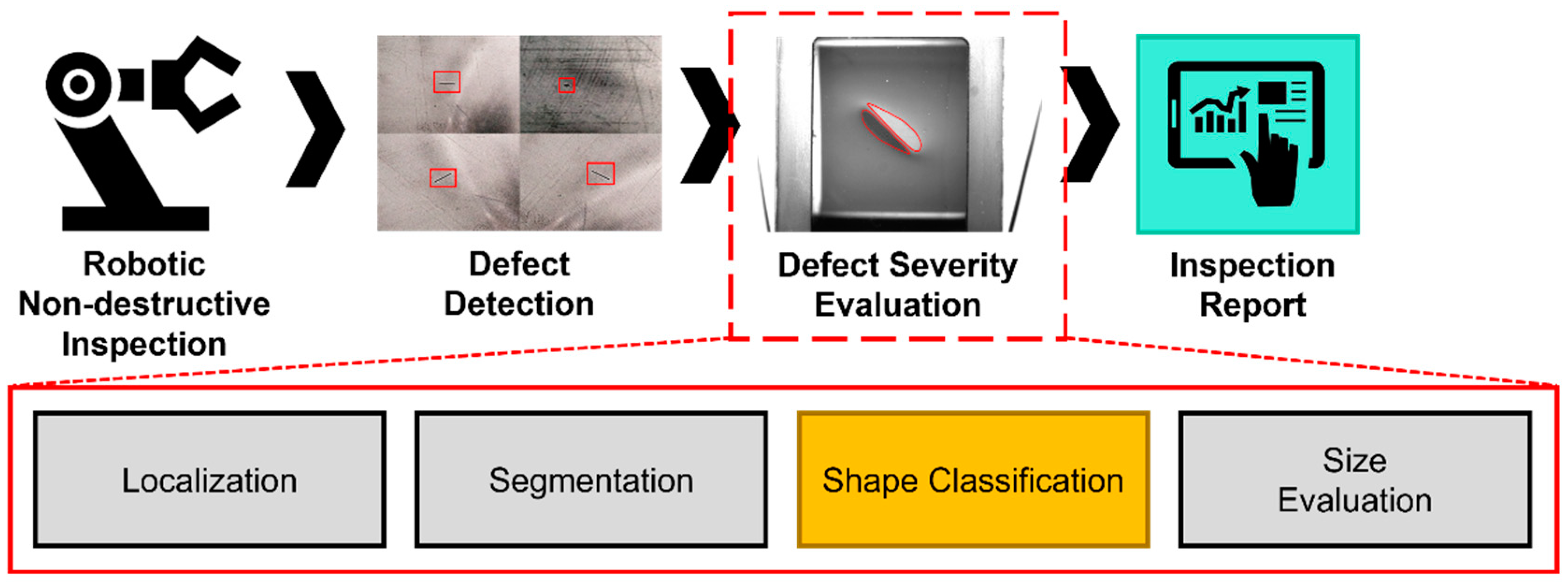
:1. Introduction
2. Materials and Methods
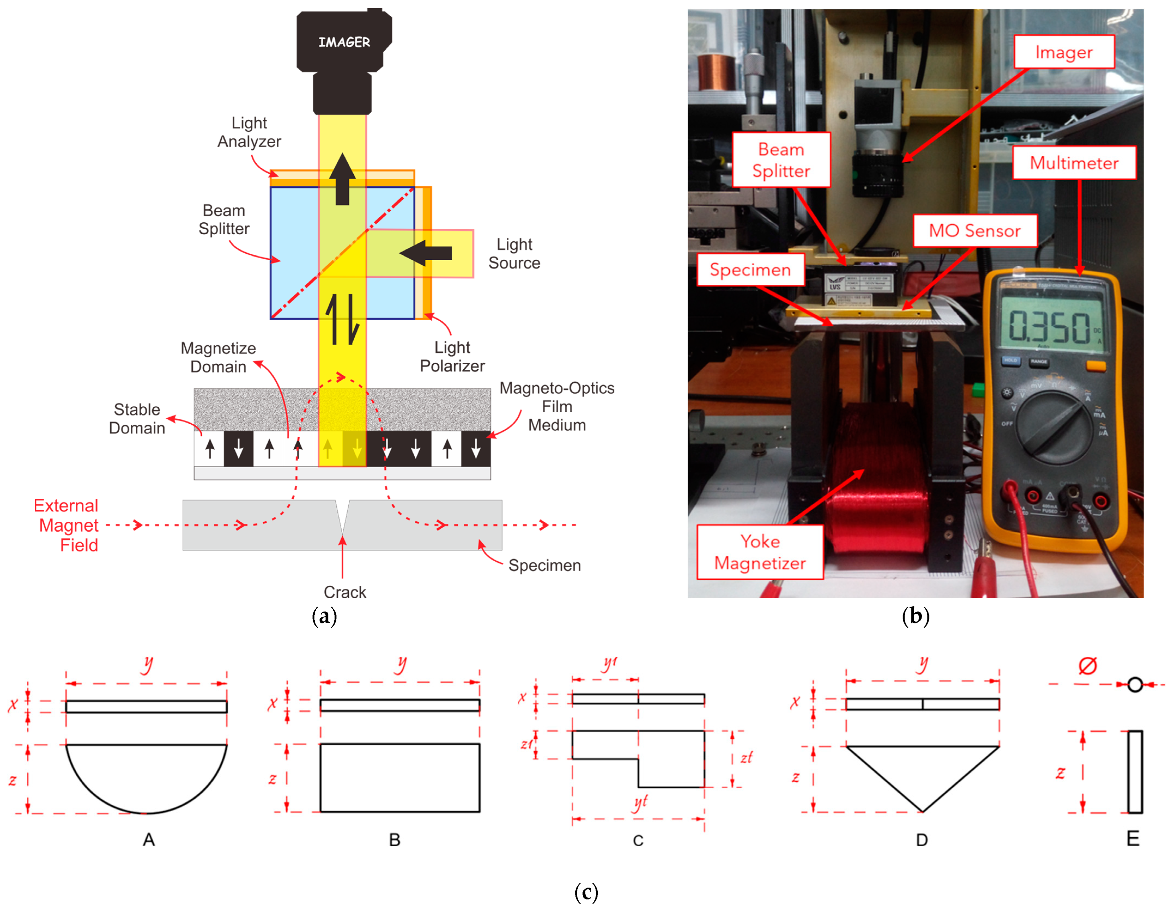
2.1. Data Acquisition
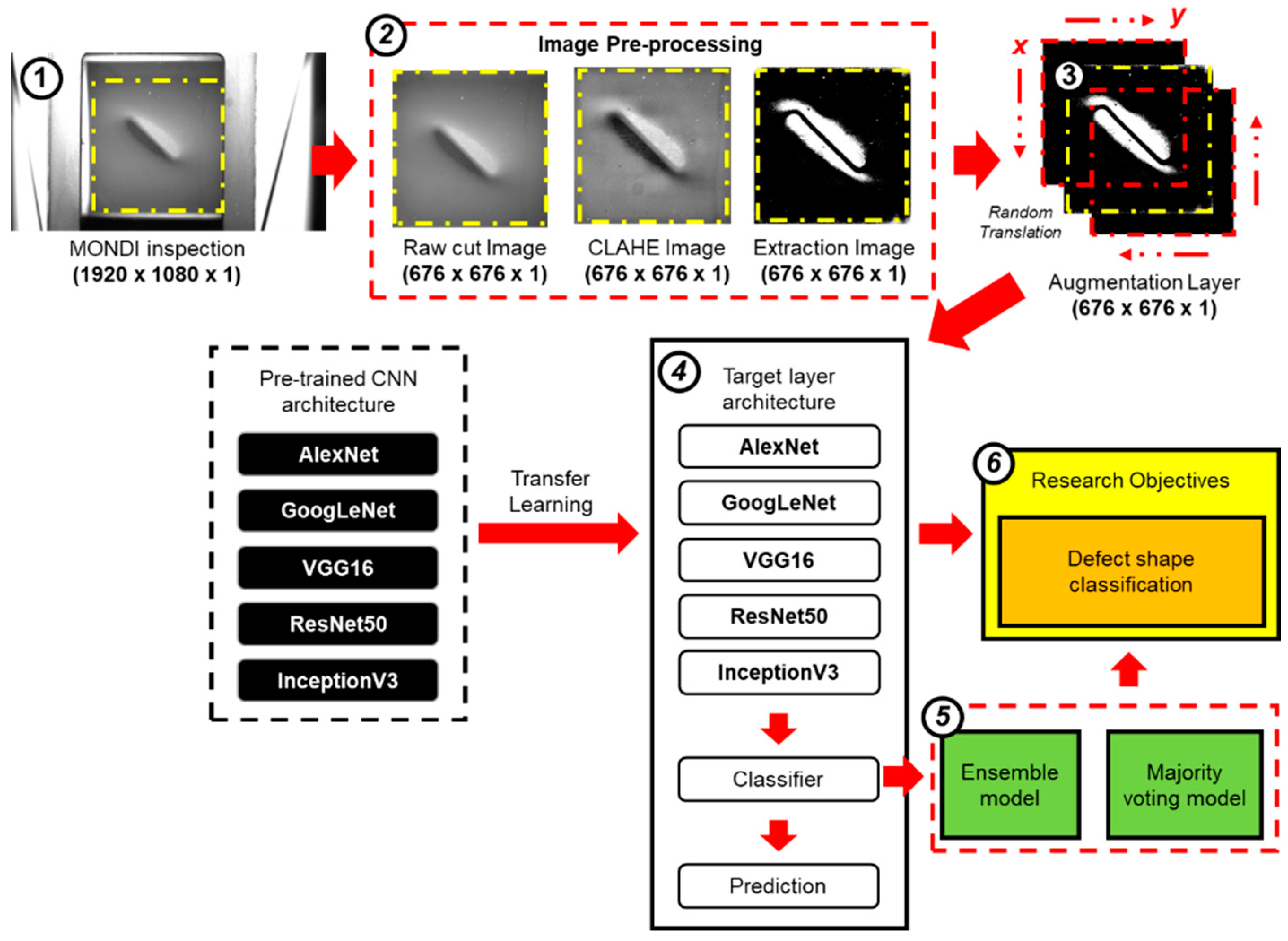
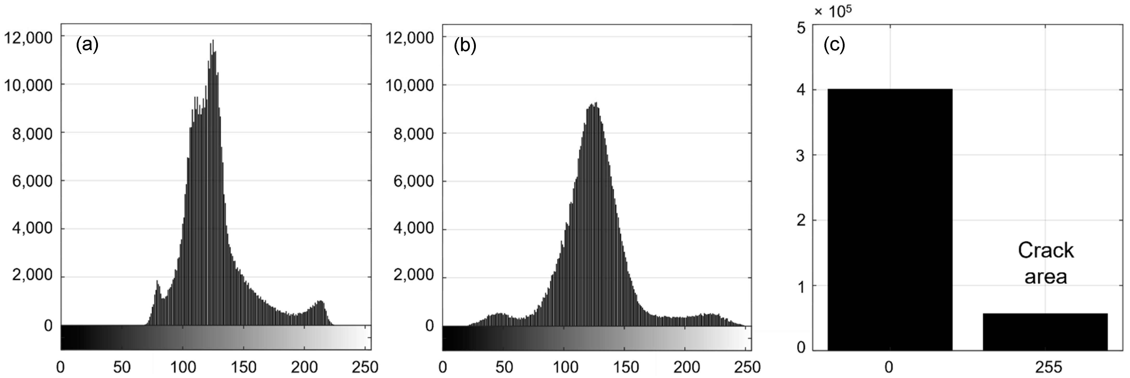
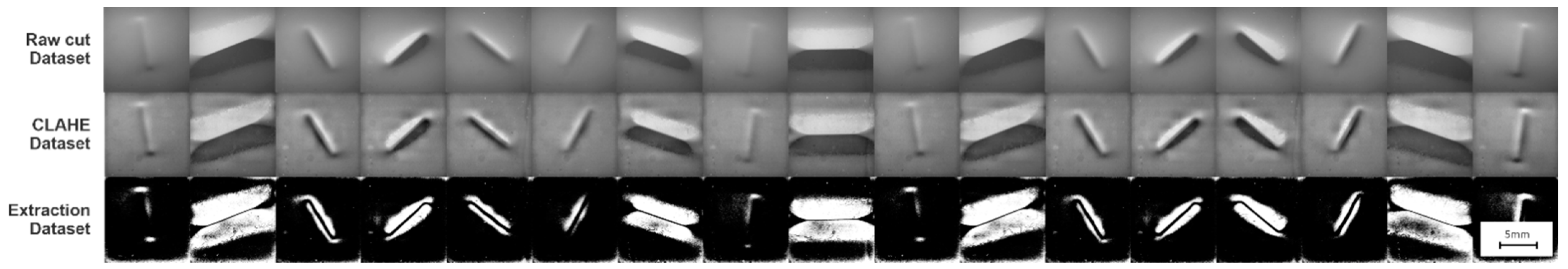
2.2. Image Preprocessing and Data Augmentation
2.3. Deep Convolutional Neural Network and Transfer Learning Pretrained Neural Network
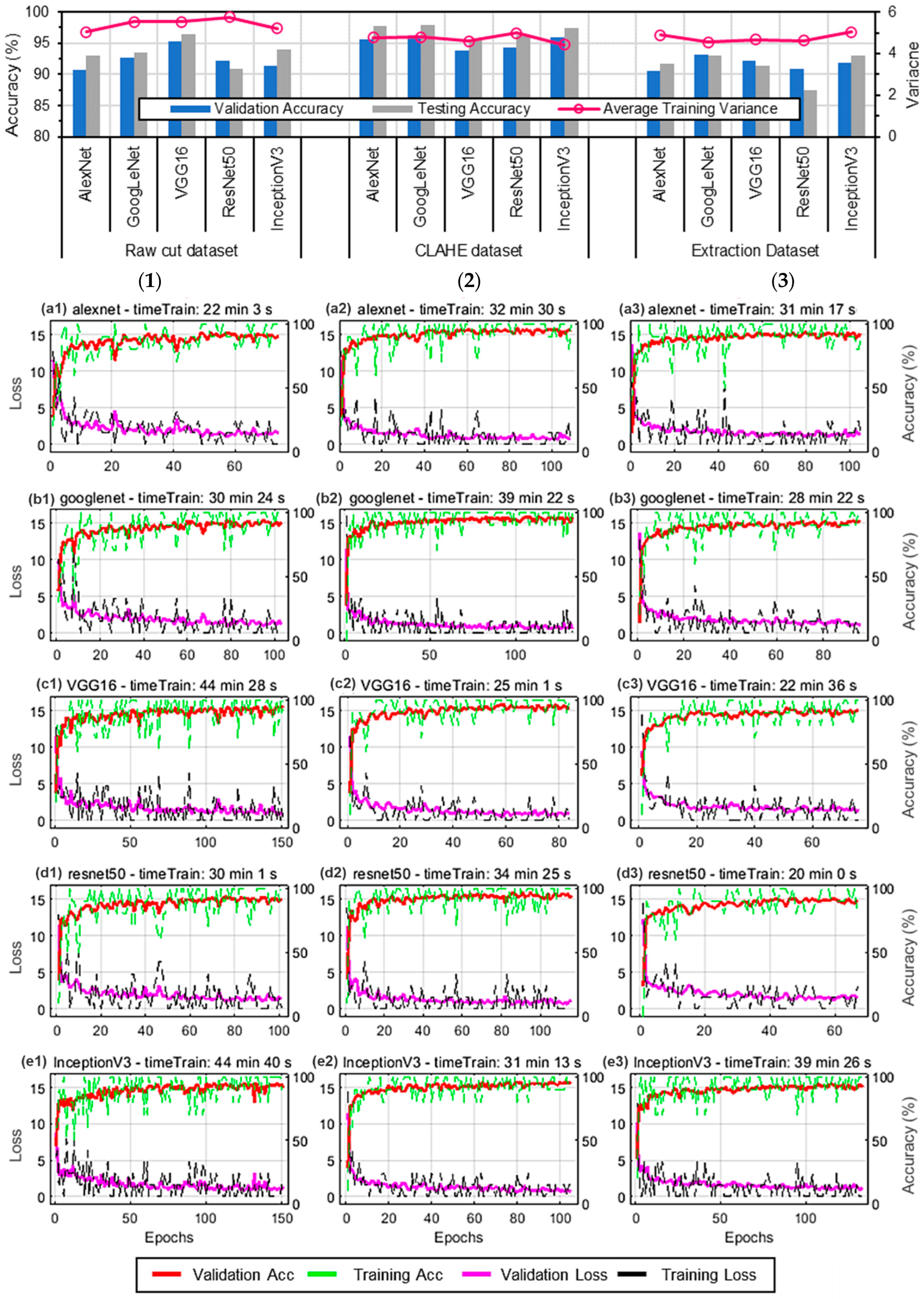
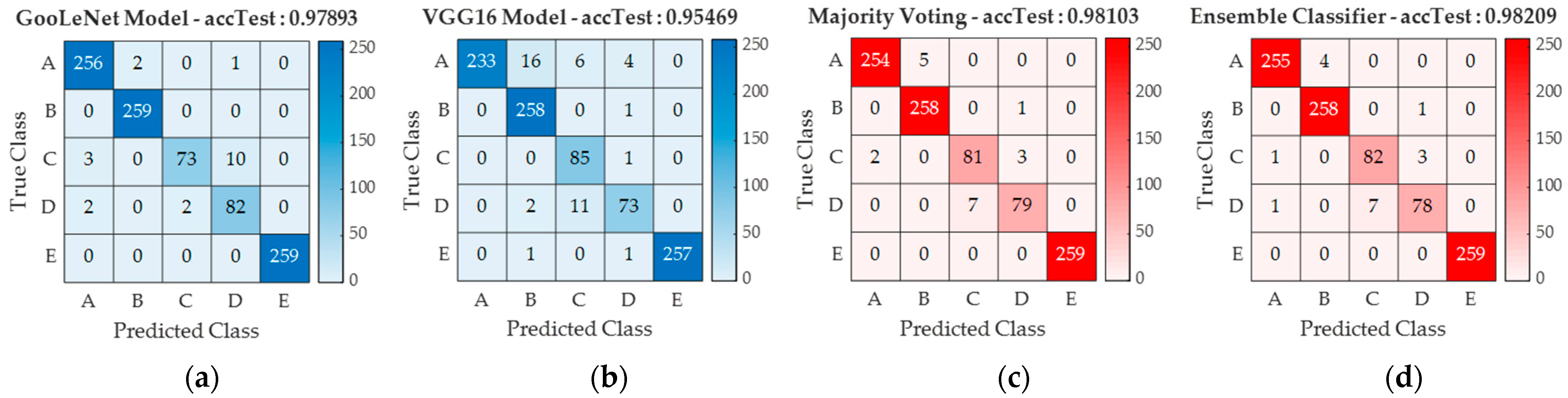
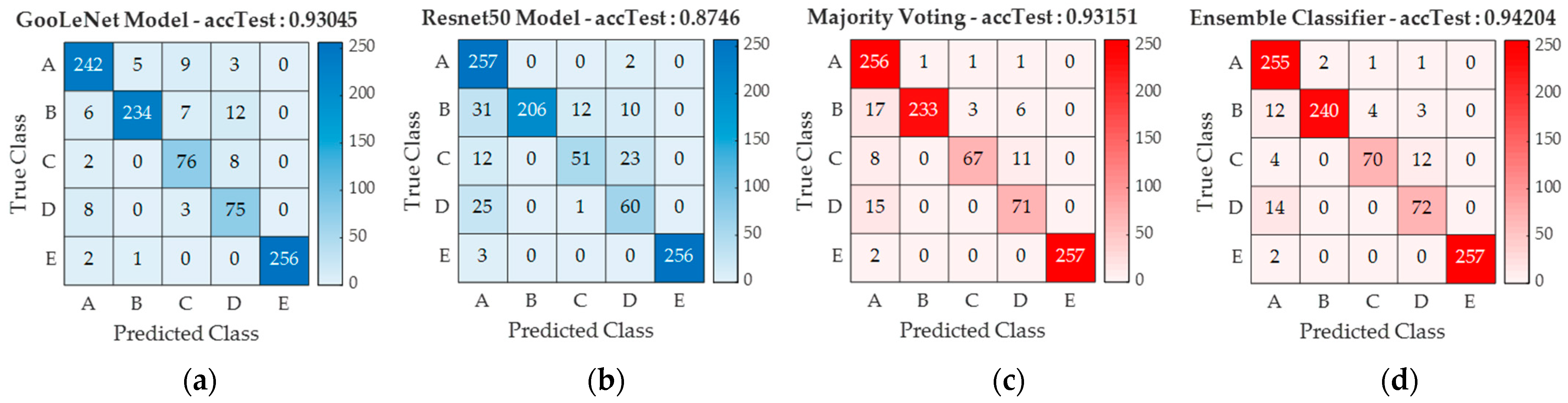
3. Experimental Results
4. Conclusions
Author Contributions
Funding
Conflicts of Interest
References
- Adamovic, D.; Zivic, F. Hardness and Non-Destructive Testing (NDT) of Ceramic Matrix Composites (CMCs). Encycl. Mater. Compos. 2021, 2, 183–201. [Google Scholar] [CrossRef]
- Pohl, R.; Erhard, A.; Montag, H.-J.; Thomas, H.-M.; Wüstenberg, H. NDT techniques for railroad wheel and gauge corner inspection. NDT E Int. 2004, 37, 89–94. [Google Scholar] [CrossRef]
- Tu, W.; Zhong, S.; Shen, Y.; Incecik, A. Nondestructive testing of marine protective coatings using terahertz waves with stationary wavelet transform. Ocean Eng. 2016, 111, 582–592. [Google Scholar] [CrossRef] [Green Version]
- Bossi, R.H.; Giurgiutiu, V. Nondestructive testing of damage in aerospace composites. In Polymer Composites in the Aerospace Industry; Elsevier: Amsterdam, The Netherlands, 2015; pp. 413–448. [Google Scholar] [CrossRef]
- Crane, R.L. 7.9 Nondestructive Inspection of Composites. Compr. Compos. Mater. 2018, 5, 159–166. [Google Scholar] [CrossRef]
- Meola, C.; Raj, B. Nondestructive Testing and Evaluation: Overview. In Reference Module in Materials Science and Materials Engineering; Elsevier: Amsterdam, The Netherlands, 2016. [Google Scholar] [CrossRef]
- Dwivedi, S.K.; Vishwakarma, M.; Soni, P. Advances and Researches on Non Destructive Testing: A Review. Mater. Today Proc. 2018, 5, 3690–3698. [Google Scholar] [CrossRef]
- Singh, R. Penetrant Testing. In Applied Welding Engineering; Elsevier: Amsterdam, The Netherlands, 2012; pp. 283–291. [Google Scholar] [CrossRef]
- Matthews, C. General NDE Requirements: API 570, API 577 and ASME B31.3. In A Quick Guide to API 570 Certified Pipework Inspector Syllabus; Elsevier: Amsterdam, The Netherlands, 2009; pp. 121–148. [Google Scholar] [CrossRef]
- Farhat, H. NDT processes: Applications and limitations. In Operation, Maintenance, and Repair of Land-Based Gas Turbines; Elsevier: Amsterdam, The Netherlands, 2021; pp. 159–174. [Google Scholar] [CrossRef]
- Goebbels, K. A new concept of magnetic particle inspection. In Non-Destructive Testing; Elsevier: Amsterdam, The Netherlands, 1989; pp. 719–724. [Google Scholar] [CrossRef]
- Rizzo, P. Sensing solutions for assessing and monitoring underwater systems. In Sensor Technologies for Civil Infrastructures; Elsevier: Amsterdam, The Netherlands, 2014; Volume 2, pp. 525–549. [Google Scholar] [CrossRef]
- Mouritz, A.P. Nondestructive inspection and structural health monitoring of aerospace materials. In Introduction to Aerospace Materials; Elsevier: Amsterdam, The Netherlands, 2012; pp. 534–557. [Google Scholar] [CrossRef]
- Lim, J.; Lee, H.; Lee, J.; Shoji, T. Application of a NDI method using magneto-optical film for micro-cracks. KSME Int. J. 2002, 16, 591–598. [Google Scholar] [CrossRef]
- Hughes, S.E. Non-destructive and Destructive Testing. In A Quick Guide to Welding and Weld Inspection; Elsevier: Amsterdam, The Netherlands, 2009; pp. 67–87. [Google Scholar] [CrossRef]
- Xu, C.; Xu, G.; He, J.; Cheng, Y.; Dong, W.; Ma, L. Research on rail crack detection technology based on magneto-optical imaging principle. J. Phys. Conf. Ser. 2022, 2196, 012003. [Google Scholar] [CrossRef]
- Le, M.; Lee, J.; Shoji, T.; Le, H.M.; Lee, S. A Simulation Technique of Non-Destructive Testing using Magneto-Optical Film 2011. Available online: https://www.researchgate.net/publication/267261713 (accessed on 24 March 2022).
- Maksymenko, O.P.; Karpenko Physico-Mechanical Institute of NAS of Ukraine; Suriadova, O.D. Application of magneto-optical method for detection of material structure changes. Inf. Extr. Process. 2021, 2021, 32–36. [Google Scholar] [CrossRef]
- Nguyen, H.; Kam, T.Y.; Cheng, P.Y. Crack Image Extraction Using a Radial Basis Functions Based Level Set Interpolation Technique. In Proceedings of the 2012 International Conference on Computer Science and Electronics Engineering, Hangzhou, China, 23–25 March 2012; Volume 3, pp. 118–122. [Google Scholar] [CrossRef]
- Lee, J.; Berkache, A.; Wang, D.; Hwang, Y.-H. Three-Dimensional Imaging of Metallic Grain by Stacking the Microscopic Images. Appl. Sci. 2021, 11, 7787. [Google Scholar] [CrossRef]
- Munawar, H.S.; Hammad, A.W.A.; Haddad, A.; Soares, C.A.P.; Waller, S.T. Image-Based Crack Detection Methods: A Review. Infrastructures 2021, 6, 115. [Google Scholar] [CrossRef]
- Lee, J.; Lyu, S.; Nam, Y. An algorithm for the characterization of surface crack by use of dipole model and magneto-optical non-destructive inspection system. KSME Int. J. 2000, 14, 1072–1080. [Google Scholar] [CrossRef]
- Xu, H.; Su, X.; Wang, Y.; Cai, H.; Cui, K.; Chen, X. Automatic Bridge Crack Detection Using a Convolutional Neural Network. Appl. Sci. 2019, 9, 2867. [Google Scholar] [CrossRef] [Green Version]
- Yang, C.; Chen, J.; Li, Z.; Huang, Y. Structural Crack Detection and Recognition Based on Deep Learning. Appl. Sci. 2021, 11, 2868. [Google Scholar] [CrossRef]
- Neven, R.; Goedemé, T. A Multi-Branch U-Net for Steel Surface Defect Type and Severity Segmentation. Metals 2021, 11, 870. [Google Scholar] [CrossRef]
- Damacharla, P.; Rao, A.; Ringenberg, J.; Javaid, A.Y. TLU-Net: A Deep Learning Approach for Automatic Steel Surface Defect Detection. In Proceedings of the 2021 International Conference on Applied Artificial Intelligence (ICAPAI), Halden, Norway, 19–21 May 2021; pp. 1–6. [Google Scholar] [CrossRef]
- Altabey, W.; Noori, M.; Wang, T.; Ghiasi, R.; Kuok, S.-C.; Wu, Z. Deep Learning-Based Crack Identification for Steel Pipelines by Extracting Features from 3D Shadow Modeling. Appl. Sci. 2021, 11, 6063. [Google Scholar] [CrossRef]
- Lee, J.; Shoji, T. Development of a NDI system using the magneto-optical method 2 Remote sensing using the novel magneto-optical inspection system. Engineering 1999, 48, 231–236. Available online: http://inis.iaea.org/search/search.aspx?orig_q=RN:30030266 (accessed on 24 March 2022).
- Rizzo, P. Sensing solutions for assessing and monitoring railroad tracks. In Sensor Technologies for Civil Infrastructures; Elsevier: Amsterdam, The Netherlands, 2014; Volume 1, pp. 497–524. [Google Scholar] [CrossRef]
- Miura, N. Magneto-Spectroscopy of Semiconductors. In Comprehensive Semiconductor Science and Technology; Elsevier: Amsterdam, The Netherlands, 2011; Volume 1–6, pp. 256–342. [Google Scholar] [CrossRef]
- Poonnayom, P.; Chantasri, S.; Kaewwichit, J.; Roybang, W.; Kimapong, K. Microstructure and Tensile Properties of SS400 Carbon Steel and SUS430 Stainless Steel Butt Joint by Gas Metal Arc Welding. Int. J. Adv. Cult. Technol. 2015, 3, 61–67. [Google Scholar] [CrossRef]
- Yadav, G.; Maheshwari, S.; Agarwal, A. Contrast limited adaptive histogram equalization based enhancement for real time video system. In Proceedings of the 2014 International Conference on Advances in Computing, Communications and Informatics (ICACCI), Delhi, India, 24–27 September 2014; pp. 2392–2397. [Google Scholar] [CrossRef]
- Kuran, U.; Kuran, E.C. Parameter selection for CLAHE using multi-objective cuckoo search algorithm for image contrast enhancement. Intell. Syst. Appl. 2021, 12, 200051. [Google Scholar] [CrossRef]
- Subramanian, J.; Simon, R. Overfitting in prediction models—Is it a problem only in high dimensions? Contemp. Clin. Trials 2013, 36, 636–641. [Google Scholar] [CrossRef]
- Gonsalves, T.; Upadhyay, J. Integrated deep learning for self-driving robotic cars. In Artificial Intelligence for Future Generation Robotics; Elsevier: Amsterdam, The Netherlands, 2021; pp. 93–118. [Google Scholar] [CrossRef]
- Teuwen, J.; Moriakov, N. Convolutional neural networks. In Handbook of Medical Image Computing and Computer Assisted Intervention; Academic Press: Cambridge, MA, USA, 2020; pp. 481–501. [Google Scholar] [CrossRef]
- Sharma, S.; Sharma, S.; Athaiya, A. Activation Function in Neural Networks 2020. Available online: http://www.ijeast.com (accessed on 24 March 2022).
- Chouhan, V.; Singh, S.K.; Khamparia, A.; Gupta, D.; Tiwari, P.; Moreira, C.; Damaševičius, R.; de Albuquerque, V.H.C. A Novel Transfer Learning Based Approach for Pneumonia Detection in Chest X-ray Images. Appl. Sci. 2020, 10, 559. [Google Scholar] [CrossRef] [Green Version]
- Zhu, W.; Ma, Y.; Zhou, Y.; Benton, M.; Romagnoli, J. Deep Learning Based Soft Sensor and Its Application on a Pyrolysis Reactor for Compositions Predictions of Gas Phase Components. In Computer Aided Chemical Engineering; Elsevier: Amsterdam, The Netherlands, 2018; Volume 44, pp. 2245–2250. [Google Scholar] [CrossRef]
- Krizhevsky, A.; Sutskever, I.; Hinton, G.E. ImageNet Classification with Deep Convolutional Neural Networks. In Advances in Neural Information Processing Systems; The MIT Press: Cambridge, MA, USA, 2012; Volume 25, Available online: https://proceedings.neurips.cc/paper/2012/file/c399862d3b9d6b76c8436e924a68c45b-Paper.pdf (accessed on 27 March 2022).
- Szegedy, C.; Liu, W.; Jia, Y.; Sermanet, P.; Reed, S.; Anguelov, D.; Erhan, D.; Vanhoucke, V.; Rabinovich, A. Going Deeper with Convolutions. In Proceedings of the IEEE conference on computer vision and pattern recognition, Boston, MA, USA, 7–12 June 2015; pp. 1–9. [Google Scholar]
- Russakovsky, O.; Deng, J.; Su, H.; Krause, J.; Satheesh, S.; Ma, S.; Huang, Z.; Karpathy, A.; Khosla, A.; Bernstein, M.; et al. ImageNet Large Scale Visual Recognition Challenge. Int. J. Comput. Vis. 2015, 115, 211–252. [Google Scholar] [CrossRef] [Green Version]
- He, K.; Zhang, X.; Ren, S.; Sun, J. Deep residual learning for image recognition. In Proceedings of the 2016 IEEE Conference on Computer Vision and Pattern Recognition (CVPR), Las Vegas, NV, USA, 27–30 June 2016; pp. 770–778. [Google Scholar] [CrossRef] [Green Version]
- Szegedy, C.; Vanhoucke, V.; Ioffe, S.; Shlens, J.; Wojna, Z. Rethinking the Inception Architecture for Computer Vision. In Proceedings of the IEEE Conference on Computer Vision and Pattern Recognition (CVPR), Las Vegas, NV, USA, 27–30 June 2016; pp. 2818–2826. [Google Scholar] [CrossRef] [Green Version]
- Zeiler, M.D.; Fergus, R. Visualizing and understanding convolutional networks. In Proceedings of the 13th European Conference on Computer Vision (ECCV), Zurich, Switzerland, 6–12 September 2014; pp. 818–833. [Google Scholar] [CrossRef] [Green Version]


| Ref. | CNN Dataset | Method | Research Objectives | Data Acquisition | Results | Novelty |
|---|---|---|---|---|---|---|
| [23] | 2068 images 1024 × 1024 pixels | CNN, atrous convolution, atrous spatial pyramid pooling (ASPP), deep-wise separable | Bridge crack detection | Phantom 4 Pro’s CMOS surface array camera | Accuracy: 96.37% Precision: 78.11% Specificity: 95.83% F1 score: 0.8771 | Random center crop operation and integrated CNN convolution |
| [24] | 2000 images 1024 × 1024 pixels | Transfer learning CNN models, YOLOv3 model | Structural crack detection | Manual photo collection and augmentation | Performance comparison and auto crack tracking with max. acc of 98.8% | YOLOv3 for crack location tracking |
| [25] | 10,000 images (4 K and 6 K) | U-Net sematic segmentation, CNN | Steel defect type, severity segmentation | Constructing manual real-life industrial dataset | Improve defect segmentation by 2.5% and severity assessment by 3% | Integrated CNN branch network |
| [26] | 12,568 images 256 × 1600 pixels | Transfer learning CNN models | Automatic steel defect detection | Public dataset | Improve defect initialization by 5% and segmentation by 26% (relatively) | Transfer learning U-Net (TLU-Net) framework for the assessment |
| [27] | 900 images 256 × 256 pixels | 3D-shadow modeling (SM), CNN | Pipelines crack identification | 3D-SM | Accuracy: 93.53% Regression rate: 92.04% | 3D-SM for pipeline defect detection |
| This study | 4752 images 676 × 676 pixels | Transfer learning CNN models | Defect shape classification | Magneto-optic nondestructive inspection (MONDI) system | Comparison of each transfer learning, ensemble, and majority voting model performance and score mapping analysis | Defect shape classification method using MONDI dataset |
| Part Number | Defect Shape | Depth (z) (mm) | Length (y) (mm) | Width (x) (mm) | Diameter (⌀) (mm) | Class | Total Image |
|---|---|---|---|---|---|---|---|
| A1 | Semioval | 1 | 4.93 | 0.5 | - | A | 432 |
| A2 | Semioval | 2 | 6.37 | 0.5 | - | A | 432 |
| A3 | Semioval | 3 | 7 | 0.5 | - | A | 432 |
| B1 | Rectangle | 1 | 7 | 0.5 | - | B | 432 |
| B2 | Rectangle | 2 | 7 | 0.5 | - | B | 432 |
| B3 | Rectangle | 3 | 7 | 0.5 | - | B | 432 |
| C | Combination | 1–3 | 3.5–7 | 0.5 | - | C | 432 |
| D | Triangle | 3 | 7 | 0.5 | - | D | 432 |
| E1 | Hole | 1 | - | - | 0.5 | E | 432 |
| E2 | Hole | 2 | - | - | 0.5 | E | 432 |
| E3 | Hole | 3 | - | - | 0.5 | E | 432 |
| Dataset | Model | Epoch | Testing Accuracy (%) | Network Accuracy (%) | Weighted Accuracy (%) | Area under the Curve (AUC) (%) | F1_Score | Classification Time (s) | ||||
|---|---|---|---|---|---|---|---|---|---|---|---|---|
| A | B | C | D | E | ||||||||
| Raw cut Image | AlexNet | 73 | 93.05 | 97.22 | 97.53 | 97.88 | 0.960 | 0.934 | 0.796 | 0.824 | 0.981 | 2.570 |
| GoogLeNet | 102 | 93.57 | 97.43 | 97.39 | 98.12 | 0.952 | 0.939 | 0.891 | 0.816 | 0.965 | 2.565 | |
| VGG16 | 150 | 96.42 | 98.57 | 98.70 | 98.70 | 0.975 | 0.972 | 0.901 | 0.901 | 0.987 | 2.570 | |
| ResNet50 | 100 | 90.94 | 96.38 | 97.44 | 97.20 | 0.967 | 0.947 | 0.688 | 0.635 | 0.990 | 2.566 | |
| InceptionV3 | 150 | 93.99 | 97.60 | 98.49 | 98.41 | 0.977 | 0.983 | 0.758 | 0.701 | 0.998 | 2.574 | |
| Majority Voting | - | 94.94 | 97.98 | 98.43 | 98.84 | 0.979 | 0.970 | 0.824 | 0.819 | 0.985 | - | |
| Ensemble | - | 95.68 | 98.27 | 98.70 | 98.84 | 0.979 | 0.976 | 0.837 | 0.849 | 0.992 | 2.608 | |
| Contrast-limited adaptive histogram equalization (CLAHE) Image | AlexNet | 109 | 97.68 | 99.07 | 99.43 | 99.32 | 0.989 | 0.996 | 0.900 | 0.889 | 1 | 2.567 |
| GoogLeNet | 133 | 97.89 | 99.16 | 99.43 | 99.06 | 0.985 | 0.996 | 0.907 | 0.916 | 1 | 2.565 | |
| VGG16 | 84 | 95.47 | 98.19 | 98.26 | 94.98 | 0.947 | 0.963 | 0.904 | 0.880 | 0.996 | 2.554 | |
| ResNet50 | 116 | 96.31 | 98.52 | 98.74 | 98.60 | 0.979 | 0.970 | 0.914 | 0.846 | 0.992 | 2.563 | |
| InceptionV3 | 105 | 97.37 | 98.95 | 99.16 | 98.31 | 0.981 | 0.985 | 0.908 | 0.912 | 0.998 | 2.563 | |
| Majority Voting | - | 98.10 | 99.24 | 99.41 | 98.89 | 0.986 | 0.989 | 0.931 | 0.935 | 1 | - | |
| Ensemble | - | 98.21 | 99.28 | 99.48 | 99.08 | 0.988 | 0.990 | 0.937 | 0.929 | 1 | 2.598 | |
| Extraction Image | AlexNet | 105 | 91.78 | 96.71 | 96.74 | 96.11 | 0.909 | 0.928 | 0.810 | 0.802 | 0.990 | 2.567 |
| GoogLeNet | 96 | 93.05 | 97.22 | 97.41 | 95.41 | 0.933 | 0.938 | 0.840 | 0.815 | 0.994 | 2.561 | |
| VGG16 | 76 | 91.36 | 96.54 | 96.71 | 95.65 | 0.910 | 0.922 | 0.797 | 0.771 | 0.996 | 2.560 | |
| ResNet50 | 67 | 87.46 | 94.98 | 95.25 | 94.47 | 0.876 | 0.886 | 0.680 | 0.663 | 0.994 | 2.567 | |
| InceptionV3 | 133 | 92.94 | 97.18 | 97.57 | 96.09 | 0.936 | 0.963 | 0.822 | 0.740 | 0.986 | 2.564 | |
| Majority Voting | - | 93.15 | 97.26 | 97.34 | 96.38 | 0.919 | 0.945 | 0.854 | 0.811 | 0.996 | - | |
| Ensemble | - | 94.20 | 97.68 | 97.82 | 96.91 | 0.934 | 0.958 | 0.869 | 0.828 | 0.996 | 2.603 | |
Publisher’s Note: MDPI stays neutral with regard to jurisdictional claims in published maps and institutional affiliations. |
© 2022 by the authors. Licensee MDPI, Basel, Switzerland. This article is an open access article distributed under the terms and conditions of the Creative Commons Attribution (CC BY) license (https://creativecommons.org/licenses/by/4.0/).
Share and Cite
Dharmawan, I.D.M.O.; Lee, J.; Sim, S. Defect Shape Classification Using Transfer Learning in Deep Convolutional Neural Network on Magneto-Optical Nondestructive Inspection. Appl. Sci. 2022, 12, 7613. https://doi.org/10.3390/app12157613
Dharmawan IDMO, Lee J, Sim S. Defect Shape Classification Using Transfer Learning in Deep Convolutional Neural Network on Magneto-Optical Nondestructive Inspection. Applied Sciences. 2022; 12(15):7613. https://doi.org/10.3390/app12157613
Chicago/Turabian StyleDharmawan, I Dewa Made Oka, Jinyi Lee, and Sunbo Sim. 2022. "Defect Shape Classification Using Transfer Learning in Deep Convolutional Neural Network on Magneto-Optical Nondestructive Inspection" Applied Sciences 12, no. 15: 7613. https://doi.org/10.3390/app12157613
APA StyleDharmawan, I. D. M. O., Lee, J., & Sim, S. (2022). Defect Shape Classification Using Transfer Learning in Deep Convolutional Neural Network on Magneto-Optical Nondestructive Inspection. Applied Sciences, 12(15), 7613. https://doi.org/10.3390/app12157613