Article

Simulation Study of a New Magnetorheological Polishing Fluid Collector Based on Air Seal

1
Faculty of Mechanical and Electrical Engineering, Kunming University of Science and Technology, Kunming 650500, China
2
Faculty of Mechanical and Electrical Engineering, Xiamen University, Xiamen 361102, China
*
Author to whom correspondence should be addressed.
Appl. Sci. 2022, 12(15), 7433; https://doi.org/10.3390/app12157433
Submission received: 21 June 2022 / Revised: 19 July 2022 / Accepted: 22 July 2022 / Published: 24 July 2022
(This article belongs to the Special Issue New Trends in Design Engineering II)

Abstract

:
Inverted magnetorheological (MR) polishing device mainly use a magnetic sealing ring to collect polishing fluid. This collection method wears the wheel surface of the polishing wheel, affects the surface accuracy of the polishing wheel, and introduces machining error. In order to reduce this wear and improve recovery efficiency, a new type of collector using an air seal is proposed in this paper. Furthermore, testing method using six factors and a three-level orthogonal test table is used to study the structural parameters of the new collector. The flow fields affected by the different structural parameters were simulated, and the corresponding collection efficiency was analyzed. The results show that the air nozzle diameter has the greatest impact on the fluctuation value of the collector outlet flow, followed by the airflow velocity and nozzle spacing. Moreover, the structural parameters obtained from the orthogonal test were optimized using the control variable method. The minimum flow fluctuation and maximum flow at the collector outlet can be obtained when the nozzle diameter is 2.5 mm and the nozzle airflow velocity is 31 m/s.

1. Introduction

MR polishing is widely used in various fields, especially in the processing of precision components, such as aerospace, biological, and precision machinery [1,2,3]. MR fluid is mainly composed of base fluid, magnetically sensitive particles, polishing abrasive particles, and a small amount of additives [4]. Under the action of the gradient magnetic field, the magnetically sensitive particles (carbonyl iron powder) in the liquid are arranged sequentially along the direction of the magnetic field, and the MR fluid transiently becomes a non-Newtonian fluid [5]. After the magnetic field is removed, the MR fluid returns to a Newtonian fluid. The process can be completed within 0.1~1 ms [6,7]. Unlike traditional polishing, MR polishing is a deterministic process characterized by efficiency, high precision, and good surface quality [8,9]. After polishing, the MR fluid is usually recovered by a magnetically sealed type of recovery. Because the magnetic field strength of the collector at the magnetic seal is greater than the magnetic field strength of the polishing wheel surface, the abrasive polishing particles in the magnetic seal are wrapped by carbonyl iron powder on the surface of the polishing wheel. During long-term processing, the polished abrasive particles at the magnetic seal seriously wear the surface of the polishing wheel. The surface contour accuracy of the worn polishing wheel is reduced, and the grooves formed by wear affect the recovery of polishing liquid, interfering with the formation of subsequent regular polishing belts and introducing processing errors, mainly intermediate frequency errors [10,11]. The oxides produced by wear also change the rheological properties of the MR fluid, reducing the cyclic service life of the MR fluid and seriously affecting the processing process.
For the simulation of MR polishing fluid, the non-Newtonian fluid viscosity model or the built-in magnetohydrodynamic model (MHD) can usually be used in simulation software. Kumar et al. [12] used COMSOL multiphysics software to analyze the computational fluid dynamics of MR fluids in the two-dimensional computational domain. The influence of different process variables on the flow variables in the processing of gear components is explored. Luo Bin et al. [13] artificially optimized the surface microstructure of the polishing disc. Based on the rheological behavior measured by MR fluid in the rheometer, a simulation model of the machining process was established in COMSOL. Manas et al. [14] used the Bingham model to simulate the two-dimensional dynamics of MR polishing fluid in a workpiece fixture. To calculate the stress generated in the polishing process, Prabhat et al. [15] simulated the formation of a polishing pad and the size of polishing pressure in chemical mechanical magnetorheological polishing. The simulation results were consistent with the experimental results obtained for aluminum alloy. Nitesh et al. [16] regarded MR polishing fluid as a Herschel–Bulkley fluid. The dynamic pressure on the workpiece surface and wall shear force at different machining clearances and velocities were calculated. Yang Hang et al. [17,18] chose the Herschel–Bulkley fluid model to replace the Bingham fluid model when studying the effect of secondary fracture surface on the formation of a pressure field in the MR polishing ribbon. The fluid model was also used to study the formation of shear stress field in the polishing entrance area. Zhang Jingjing [19] simulated the magnetic field in the Maxwell model and loaded the results into simulation software to realize the simulation of MR plane polishing. Gao Shang [20] imported a staggered arrangement of permanent magnet ferromagnetic induction intensity into simulation software. The two-phase flow characteristics of MR polishing liquid in the polishing process were simulated. Both simulation methods of MR polishing fluid have been widely used and verified. Therefore, it can be selected according to demand.
Many scholars have studied the wear if the polishing wheel in MR polishing. Some scholars have researched the material of the polishing wheel to enhance the wear resistance. Zhang Zujun et al. [21] took stainless steel as the base material, Ni-W-P as a hard alloy, and added wear-resistant particles, such as silicon carbide and hexagonal boron nitride, to coat the surface of the polishing wheel, and the wear resistance of the coating was 5.22 times that of 0Cr18Ni9Ti stainless steel. He Jihua [22] used microarc oxidation technology to treat the surface of an LY12 aluminum polishing wheel and investigated the wear resistance of the ceramic film prepared by with optimal process parameters of the aluminum substrate, as well as the constant pressure and constant current mode in the MR fluid. The results showed that under a load of 5 N, the constant pressure film exhibited wear failure after 12 min. With an extension of friction time, the amount of wear on the aluminum substrate increased linearly, and the wear rate of the constant-current film increased slowly.
Other scholars studied the collectors and wear mechanism of the polishing wheel. Kordonski [23] first designed a magnetic seal device to collect MR fluid, which is widely used today. Dong Guozheng [24] designed a recovery device with soft a magnetic stripe in the small-diameter MR polishing device. The soft magnetic stripe with a magnetic induction intensity of 0.02 T was adhered to the opening of the collection pipe, which resolved the problem of the polishing liquid not being fully recovered. Lu Jingyu [25] used a scraper to collect MR polishing fluid in the inverted polishing device. The scraper scraped the polishing solution into the collector and pumped it into the recycling pool to stir evenly. Wang Anwei [26] designed a U-shaped scraper collector with an opening consistent with the shape of the polishing wheel. The collector was coated with Tefluron or similar wear-resistant materials at the U-shaped port to improve its service life. Wang Daowen [27] designed a collection method consisting of a built-in magnet to reduce the wear on the polishing wheel. The magnet was located inside the polishing wheel, and the magnetic field intensity was greater than that of the built-in magnet in the collector, which can keep the abrasive polishing particles in the magnetic seal away from the polishing wheel. Li Yue et al. [28] established a semifixed abrasive wear model of the polishing wheel and analyzed the influence of different factors on the wear of the polishing wheel. The experimental results showed that the wear rate decreased with increased clearance of the recycler and first increased before decreasing with increased rotational speed of the polishing wheel. He [29] also proposed a collection method comprising presetting MR elastomers without abrasive polishing particles at the magnetic seal of the collector. After polishing for 5 h, the wear rate of the presetting magnetic seal polishing wheel was 0.2 mg/h, which was less than that of the working magnetic seal (1.2 mg/h).
Although the above solutions reduce wear on the polishing wheel to a certain extent, it is not eliminated altogether due to the use of traditional magnetic force and a scraper seal. In this paper, a new collector using an air seal is developed. First, the geometric structure of the new collector was presented. Second, a fluid simulation model of the new collector was set up. Thirdly, the structural parameters of the new collector were studied using six-factor and three-level orthogonal experimental design method. By analyzing the fluctuation value of export mass flow and recovery efficiency, the optimal structural parameters were obtained. On the basis of the orthogonal test, the control variable method was used to further optimize the structural parameters.

2. Geometric Structure of MR Polishing Collector

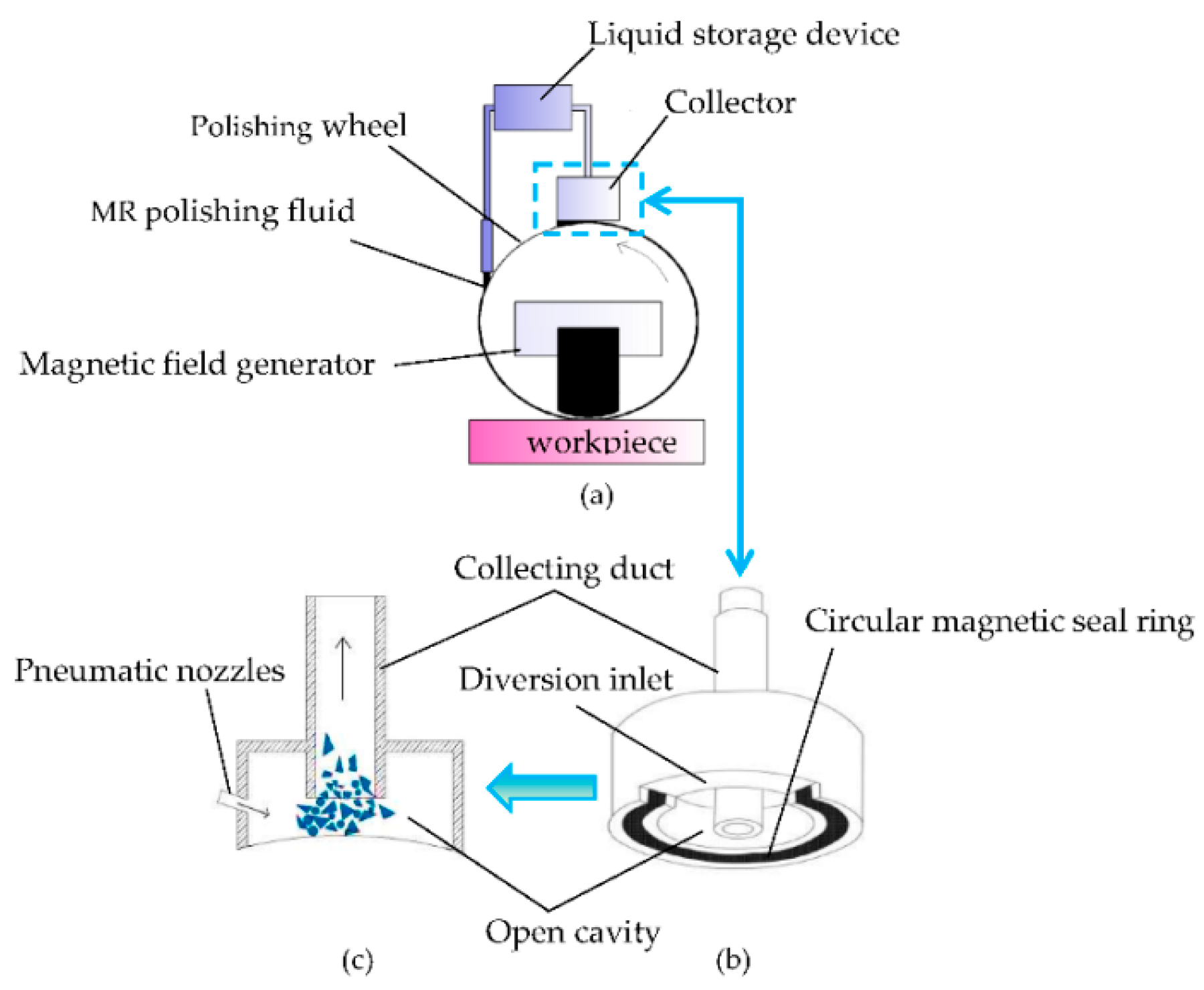
2.1. Principle of MR Polishing Liquid Collection

A sketch of a magnetorheological polishing device is shown in Figure 1a. The polishing fluid flows on the surface of the polishing wheel; then, the polishing fluid is controlled by the magnetic field generator to polish the workpiece. After polishing, the polishing fluid is returned to the collector by the polishing wheel. A traditional collector is shown in Figure 1b. The collector has a circular magnetic seal ring. The used polishing fluid is brought into the open cavity of the collector through the diversion inlet by hindering the circular magnetic seal ring. Then, the polishing liquid in the open cavity is inhaled by the negative-pressure air through the collecting duct. As mentioned above, serious wear of polishing wheel occurs when using a circular magnetic seal. Thus, a new air seal collector is developed here. Figure 1c shows a sketch of the proposed collector. Pressurized air is projected into the open cavity through pneumatic nozzles to hinder the polishing fluid. Pressurized air serves as an alternative to the circular magnetic seal ring to prevent the polishing liquid from flowing out of the open cavity along the polishing wheel.
Figure 2 shows a traditional collector and air-sealed collector. Figure 2a,b are depictions of traditional collectors, whereas Figure 2c is the new air-sealed collector. The difference between the three is that the traditional collector uses a magnetic seal and scraper for collection, whereas the new collector is based on the nozzle forming an airflow seal for collection.

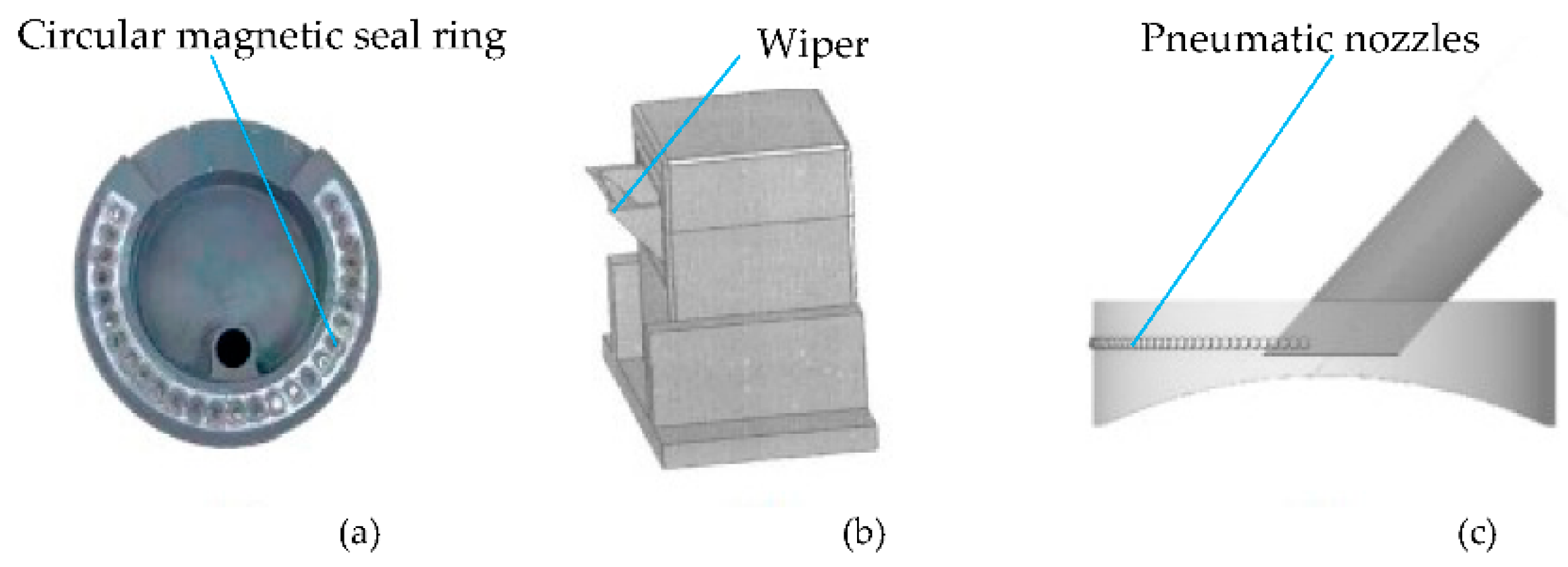
2.2. Geometric Parameters of Airflow Seal Collector

In this paper, the collector model is appropriately simplified; the corresponding interaction between each part of the collector model and the actual component is shown in Figure 3. There is a small gap between the collector and the polishing wheel, which simplifies the polishing wheel and the collector as a whole, and the polishing wheel surface is the bottom of the model arc. The polishing belt is simplified as a fixed-size fluid inlet in the model.
The geometry of the simplified collector is shown in Figure 4. The diameter of the collector cavity is 120 mm, and the height is 32 mm. The diameter of the collector duct is 25 mm, and the radius of the curved surface is 150 mm. The polishing liquid on the wheel surface is regarded as a regular ribbon. The right end of the model shown with a fixed structural size. The width is 10 mm, and the height is 1.3 mm.

3. Simulation Parameters of MR Polishing Liquid Collector

3.1. Fluid Control Equation

The commercial software FLUENT is used to simulate and analyze the airflow seal collection of MR polishing fluid. MR polishing fluid contains a large number of magnetically sensitive particles and abrasive polishing particles, which can be regarded as a solid–liquid multiphase flow. The particle group is regarded as a quasi-fluid, and the fluid is regarded as a continuous medium. It is assumed that the solid particles are uniformly distributed in the fluid, with continuous velocity field and temperature field [30].
A mixture multiphase flow model is used to simulate the movement of each phase fluid. The continuous equation of MR polishing fluid is [31]:
t ( ρ m ) + ( ρ m ν m ) = 0
t ( ρ m ν m ) + ( ρ m ν m ν m ) = p + [ μ m ( ν m + ν m T ) ] + ρ m g m + F + ( k = 1 n α k ρ k ν d r , k ν d r , k )
where ρ is mixed density, ν m is the average mass velocity, μ m is the mixed viscosity coefficient, F is volume force, α k is the volume fraction of phase k, ρ k is the density of phase k, ν m dr , k is the phase k drift velocity, and F is the source term of magnetic force after applying a magnetic field to the MR polishing fluid.
Assuming that the magnetically sensitive particles are ideally spherical, the magnetic dipole moment under the magnetic field condition is:
m = ν M = ν 3 ( μ μ 0 ) ( μ + 2 μ 0 ) H
M = χ H = χ 1 + χ μ 0 B
The magnetic force is:
F = ( m ) B
where ν is the volume of carbonyl iron powder, M is the magnetization of carbonyl iron powder, χ is magnetic susceptibility, μ is the relative permeability of carbonyl iron powder, μ 0 is vacuum permeability, and B is the magnetic induction intensity of carbonyl iron powder.

3.2. Simulation Parameters

The mixed phases used in the simulation are deionized water (DW), carbonyl iron powder (CIP), and cerium oxide (CeO2). The density, particle size, permeability, and volume fraction of each phase are shown in Table 1.
The magnetic field distribution of the model is shown in Figure 5. Because the magnetic field intensity at the MR collector is less than that in the polishing area, the rheological properties of the polishing liquid in this area are weak, changing the viscosity properties of the material is not necessary. The MHD module built in FLUENT can be used to simulate the apparent change in the polishing liquid under the conditions of a uniform magnetic field. A magnetic induction intensity of 0.01 T [32,33] is applied to the flow area of the polishing liquid, and the magnetic field direction is positive along the Y axis.
Reynolds number is an infinite number that determines whether the fluid flow is laminar or turbulent. The definition is as follows:
Re = ρ vd μ
where ρ is the density of the fluid, v is the velocity of the fluid, d is the characteristic scale of flow field, and μ is the viscosity coefficient of the fluid. The critical Reynolds number, Re cr = 2100 , is used as the criterion. There are multiple fluid phases in the simulation model, resulting in different Reynolds numbers in different fluid regions. The air density is 2.225 kg/m3, the velocity is 30 m/s, the characteristic scale is the nozzle diameter of 0.002 m, and the aerodynamic viscosity is 1.7894 × 10⁻⁵. According to Formula (6), the Reynolds number at the airflow nozzle is 4083 > 2100, which is turbulent. MR polishing fluid at the entrance can be used as a turbulence treatment. When MR fluid is affected by the magnetic field, the viscosity of the polishing fluid changes. The polishing fluid adheres to the surface of the polishing wheel and is laminar.
The simulation solver type is a pressure base solver, the time format is transient, the time integration scheme is implicit integration, and the interface modeling is phased local discretization. As the Reynolds number is greater than the critical number, a realizable k-epsilon turbulence model is selected. The momentum equation, kinetic energy equation, and kinetic energy dissipation rate are calculated by the first-order upwind scheme and SIMPLE algorithm. The calculation time step is 4 × 10³, and the final simulation time is 1 s. Considering the influence of gravity, the gravity acceleration along the negative direction of the Y axis is set to 9.8 m/s. The polishing wheel surface is set as the rotating wall. The center of the rotation is the center of the curvature of the surface (0,−138.48,0). The direction of the rotation axis is counterclockwise along the Z axis, and the speed is 110 r/min. In order to make the simulation test closer to the actual situation, the linear velocity of the inlet boundary of the MR polishing liquid is applied at the same speed as that of the polishing wheel, and the non-slip wall is selected, i.e., it is assumed that the polishing liquid has no relative slip velocity with the wheel surface. The collector outlet is connected to the recovery pump, and the pressure is negative 0.2 MPa.

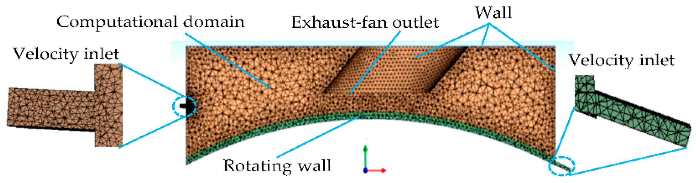
3.3. Boundary Conditions and Meshing

The mesh and boundary conditions of the model are shown in Figure 6. The mesh is automatically divided by the FLUENT mesh module. The irregular three-dimensional geometry can be divided into tetrahedral meshes by this method. The inlets of the air flow nozzle and MR polishing fluid are set as velocity inlets, and the collecting duct is the outlet of the exhaust fan. The lower surface of the collector is a rotating wall, and the rest are wall boundary conditions. The quality distribution of the model grid is shown in Figure 7. Taking Model 1 in the orthogonal experiment as an example, the grid cells size is 1.2 mm, the total number of grid cells is 1,177,591, and the number of grid nodes is 22,932. The grid mass of Model 1 is mostly distributed in the range of 0.5–1. The minimum grid quality is 0.158, accounting for 0.0009%, and the maximum grid quality is 0.956, accounting for 24%. In order to carry out accurate simulation, the average cell mass of the grid cannot be less than 0.7 [34], and the average cell mass of the grid in Model 1 is 0.838, which meets the cell mass requirements for precise simulation.

4. Experimental Design Using an Orthogonal Table

4.1. Evaluation Indices of Collection Effect

The collection process of MR polishing fluid is transient, enabling monitoring of the mass flow of the collector outlet and intuitive characterization of the collection effect of different models. Moreover, taking the fluctuation value of the mass flow of the outlet within 0.3 s as the evaluation index, the interference caused by retention of the polishing fluid in the collector can be effectively eliminated. Equation (7) is the calculation method of outlet flow fluctuation:
Δ Q m = Q max Q min
where Q max is the maximum mass flow, Q min is the minimum mass flow, and Δ Q m is the fluctuation value of outlet mass flow. A low Δ Q m value indicates that the collection effect is good with minimal fluctuation of the outlet flow, and the corresponding collector structure parameters are also optimal.

4.2. Design of Orthogonal Test Table

The polishing fluid can enter the collector cavity because the arc magnet of the magnetically sealed collector is semicircular. Similarly, too many nozzles hinders the polishing liquid from entering the collector cavity. Therefore, the number of nozzles selected for simulation is 69, only considering the influence of nozzle spacing.
Figure 8 is a schematic diagram of the influencing factors of the model. In the previous simulation, it was found that the gas nozzle inclination (φ), nozzle diameter (D), nozzle spacing (θ), relative height of the collection tube (L), collection tube inclination (α), and the nozzle airflow velocity (V) affect the collection of MR polishing fluid.
After determining six factors, a six-factor, three-level orthogonal table L18(36) is designed for simulation testing. The level of factors selected by the orthogonal table is shown in Table 2. Factor 1 is the nozzle inclination angle, which is the angle between the nozzle and the flow direction of the polishing liquid. Factor 2 is the nozzle diameter. Factor 3 is the nozzle spacing, which is the radian value between adjacent nozzles. Factor 4 is the distance between the collection tube and the polished wheel surface. Factor 5 is the inclination of the collector tube, which is the angle between the collector tube and the upper end face of the collector. Factor 6 is the air velocity.
In Table 2, the selection principle of factor levels is as follows: The nozzle inclination affects the gas-sealing effect, and three inclination angles of 3°, 6°, and 9° should be considered. The choice of nozzle diameter should not be too small; the small aperture is not easy to process, and excessive air flow generates heat and noise, so D is set as ≥ 1 mm. In terms of the choice of nozzle spacing, a value that is too low causes the nozzles to interfere with one another, whereas excessive spacing does not allow for effective formation of a gas seal; therefore, spacing is set as 2 ≤ θ ≤ 5. There is a gap of 2–3 mm between the collector and the polishing wheel and a gap of 1–2 mm between the collector and the polishing fluid. However, if the collection tube is too high, the polishing liquid cannot be collected, so the height is set as 5 mm ≤ L ≤ 10 mm. The jet velocity of the nozzle is too small to separate the polishing solution from the surface of the polishing wheel, so V ≥ 25 m/s is adopted.

4.3. Results and Discussion of Orthogonal Test

Figure 9 is a simulation cloud chart of model 1 in the orthogonal test. In the chart, the MR polishing fluid has a regular polishing ribbon on the wheel surface, which is the same as the actual working condition. The polished ribbon is gradually narrowed by airflow agglomeration at the exit and is sucked out by negative pressure. The uniform boundary conditions and grid unit size are used in the collection model, and the simulation data are directly extracted. The mass flow of polishing liquid is positive in the calculation domain and negative in the outflow.
Figure 10 shows the variation in outlet flow of each model with time, from which the increase in mass flow of the collector outlet of 1 to 18 groups of models under air seal collection can be observed. Low exit flow is monitored at the exit of the collector after t = 0 s, and there are differences between the models. The main reason is that in order to improve the iterative speed and ensure the stability of the calculation, the multiphase flow model is used as a mixed model in the simulation calculation, and the influence of the initial value of the calculation domain is given by the standard initialization. In addition, the continuous effect of the airflow can blow and disperse the liquid on the surface of the polishing ribbon in the collector, and a small amount of polishing liquid can also be collected. After t = 0.05 s, the MR polishing fluid has reached the bottom of the collection port driven by the polishing wheel. Under the negative pressure of the collection tube, the polishing fluid can be continuously collected, so the fluctuation of the outlet flow is small and shows a relatively gentle state.
Figure 11 shows the variance of the model outlet flow rate. Furthermore, the fluctuations of models 1, 2, 7, 13, and 14 are large, which implies that the collection effect of these five models is poor.
Table 3 shows the range analysis results of orthogonal testing. The primary and secondary factors of mass flow at the collector outlet are D > V > φ≈α > L > θ, which shows that the diameter of the gas nozzle has the greatest influence on the collection of polishing liquid, followed by the airflow velocity of the nozzle, and the influence of nozzle spacing is the smallest. The inclination of the gas nozzle and the inclination of the collecting duct have the same influence on the stable collection of polishing liquid.
The effect curve in Figure 12 show that with an increase in nozzle inclination, the fluctuation value of mass flow at the collector outlet first increases and then decreases. When the nozzle diameter increases, the fluctuation value decreases, indicating that there is an optimal diameter to obtain the best polishing liquid collection effect. Factors 3 to 5 meet the minimum fluctuation requirements, and there is no obvious change in regularity. When the airflow velocity is 30 m/s, the outlet flow fluctuation value is the lowest, and a velocity between 30 and 35 m/s results in the best collection effect of the polishing liquid.
The level 3-3-1-1-1-1-2 in Table 3 is the best combination, so the best combination of this orthogonal experiment is φ-9, D-2, θ-2.5, L-5, α-45, V-30.
Table 4 shows the variance analysis results of Δ Q m (fluctuation value), which further determines the significant influence of each factor on the smooth collection of MR polishing solution (F0.05(2,5) = 5.79, F0.01(2,5) = 13.27). At the confidence level of 95%, the F values of factor 2 and factor 6 are 12.812 and 8.718, respectively, which are greater than F0.05(2,5) but less than F0.01(2,5), indicating that factor 2 and factor 6 have significant indigenous effects on. Δ Q m , with contribution rates of 44.345% and 28.976%, respectively. Factors 1, 3, 4, and 5, statistic F values less than F0.05(2,5), have no significant effect.
The outlet mass flow of the model is shown in Figure 13. Within 0.1 s–0.4 s, the outlet flow is relatively stable, which is maintained at about 0.1 kg/s. Under the continuous effect of airflow, the polishing solution fluctuates slightly within the range of 0.5 s–0.7 s, and the hindering effect of airflow on the polishing solution is significantly enhanced.
A portion of the MR polishing fluid is dispersed in the collector by airflow during the collection process of the airflow seal, which leads to varying degrees of fluctuation of outlet mass flow. The percentage of collector outlet mass flow and inlet mass flow at different times are defined as instantaneous collection efficiency. The instantaneous collection rate is calculated as (8):
Q η = Q o Q i × 100 %
where Q η is the instantaneous collection efficiency, Q i is the inlet flow rate, and Q o is the outlet flow rate. In the equation, if the outlet flow rate is less than the inlet flow rate at a given moment, the fluid is poorly collected and there is a large amount of polishing fluid that is not collected. On the contrary, when the outlet mass flow rate is greater than the inlet flow rate, the collection effect is considered good. An instantaneous collection efficiency of more than 100% can be interpreted as the result of the polishing solution remaining in the collector at a given moment during collection.
As shown in Figure 14, the instantaneous collection efficiency in this period decreases to 62.4%, which is the lowest outlet flow in 1 s calculation time.

5. Model Optimization and Analysis

5.1. Optimization of Air Nozzle Diameter

The optimal model is obtained by orthogonal test analysis. From Figure 12 shows that factors 2 and 6 have optimal values. At present, the other factor levels of the optimal model are fixed, and the influence of nozzle inclination and diameter on the collector outlet flow is explored by controlling variables.
Figure 15a is the mass flow of the collector outlet when the nozzle diameter increases to 2.5 mm, 3 mm, 3.5 mm, and 4 mm. Figure 15a shows that with increased nozzle diameter, the mass flow of the collector outlet fluctuates in different ranges, with the greatest fluctuation when the nozzle diameter is 4 mm and the average flow of the corresponding outlet is the lowest. The fluctuation of the outlet flow of at 3 mm diameter is small, but it shows a downward trend. The fluctuation at 3.5 mm and 2.5 mm is moderate, indicating a good collection effect.
Figure 15b is the best model outlet average mass flow. With increased nozzle diameter, the average mass flow of the collector outlet decreases. When the nozzle diameter is 2.5 mm, the outlet flow is the highest, and when the nozzle diameter is 4 mm, the outlet flow is the lowest.
Compared with the average mass flow at the outlet of the optimal model in Figure 15b, when the diameter is 2.5 mm, the average outlet flow increases, and as the nozzle diameter increases, the average flow decreases significantly. When the diameter is 4 mm, the average flow decreases to 0.066 kg/s.
V = Q / F
where V is the nozzle airflow velocity, Q is gas flow, and F is the nozzle cross-sectional area. According to the relationship between gas flow and the cross-sectional area in Equation (9), the airflow velocity remains unchanged. With increased nozzle cross-sectional area, the gas flow at the nozzle outlet increases, the gas pressure acting on the unit area of MR polishing liquid decreases, and the polishing liquid is enhanced by the discrete effect. Therefore, with increased nozzle diameter, the flow at the collector outlet shows a downward trend as a whole. Therefore, 2.5 mm is the optimal nozzle diameter.

5.2. Optimization of Airflow Velocity

The effect of airflow velocity on MR polishing fluid collection is also obvious. On the basis of selecting a 2.5 mm nozzle diameter and changing the nozzle airflow speed, the collector outlet flow is shown in Figure 16.
As shown Figure 16a, the change in airflow velocity has little effect on the fluctuation of collector outlet flow, and it is relatively stable. Figure 16b shows that with increased airflow velocity, the average flow rate gradually decreases. When the airflow velocity is 31 m/s, the average flow rate of the outlet is the highest, reaching 0.095 kg/s. When the airflow velocity is 34 m/s, the flow rate decreases to 0.075 kg/s. Excessive airflow velocity reduce the collection efficiency of the MR polishing solution, so 31 m/s can be taken as the optimal airflow velocity.

5.3. Simulation Analysis of Optimal Polishing Liquid Collection Model

The influence of the model obtained by orthogonal experimentation and the optimized model on the collection effect of polishing liquid was compared and analyzed. With the other structural parameters unchanged, the nozzle diameter is 2.5 mm, and the airflow velocity is 31 m/s for the simulation model. In the 0.6 s collection time, the outlet flow values at different times are taken with equal spacing. The results are shown in Figure 17. As shown in Equation (7), within 0.1–1 s, the fluctuation value of the collector outlet flow is 0.079 before optimization and 0.077 after optimization. The average export mass flow after optimization is 0.081 kg/s, which is greater than the 0.078 kg/s before optimization. There is little difference between the two, but the fluctuation value of the model optimized by the control variable is lower. Therefore, the optimized nozzle diameter and airflow velocity can be used as the optimal parameters of airflow seal collection.

6. Conclusions

In this paper, a new type of MR polishing liquid collector with air-sealed collection was proposed, and an orthogonal test table was designed to explore the influence of different structural parameters on the collection effect. On the basis of the optimal model obtained by orthogonal testing, according to the main effect diagram of the factor, the control variable method was used to further optimize the orthogonal factor, and the following conclusions were obtained:
(1)
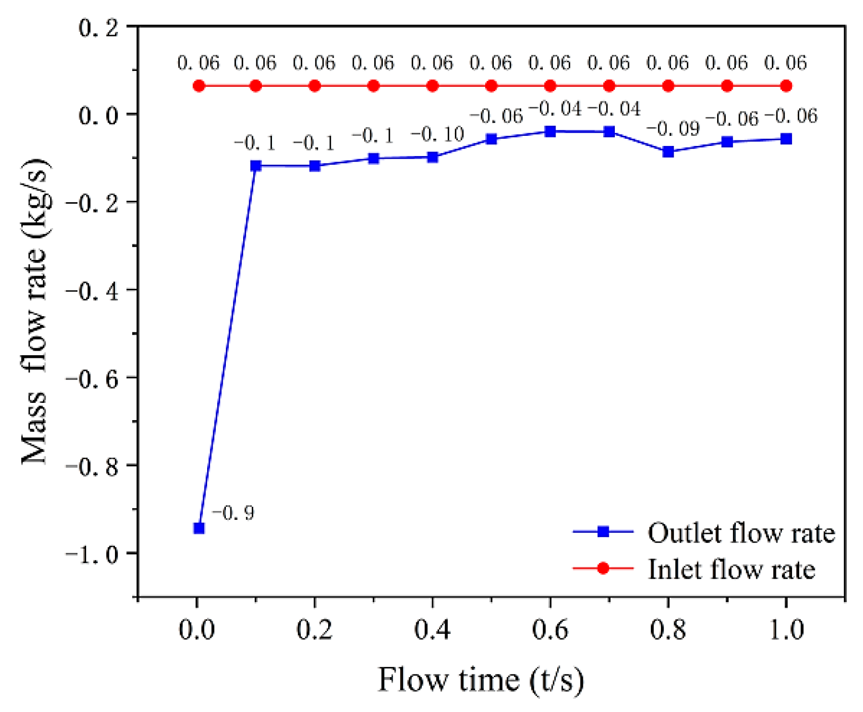
MR polishing fluid can be rapidly collected under the combined action of the collector nozzle airflow pressure and outlet negative pressure. At 0.05 s, the outflow of polishing fluid is monitored at the collector outlet, which effectively shortens the wear time of cerium oxide abrasive particles in the MR polishing fluid on the polishing wheel.
(2)
In the case of 69 nozzles used in the collector simulation model, the orthogonal test results show that the main factor affecting the fluctuation of outlet flow of different MR polishing liquid collectors is the diameter of the airflow nozzle, followed by the airflow velocity of the nozzle, and the influence of nozzle spacing is the smallest.
(3)
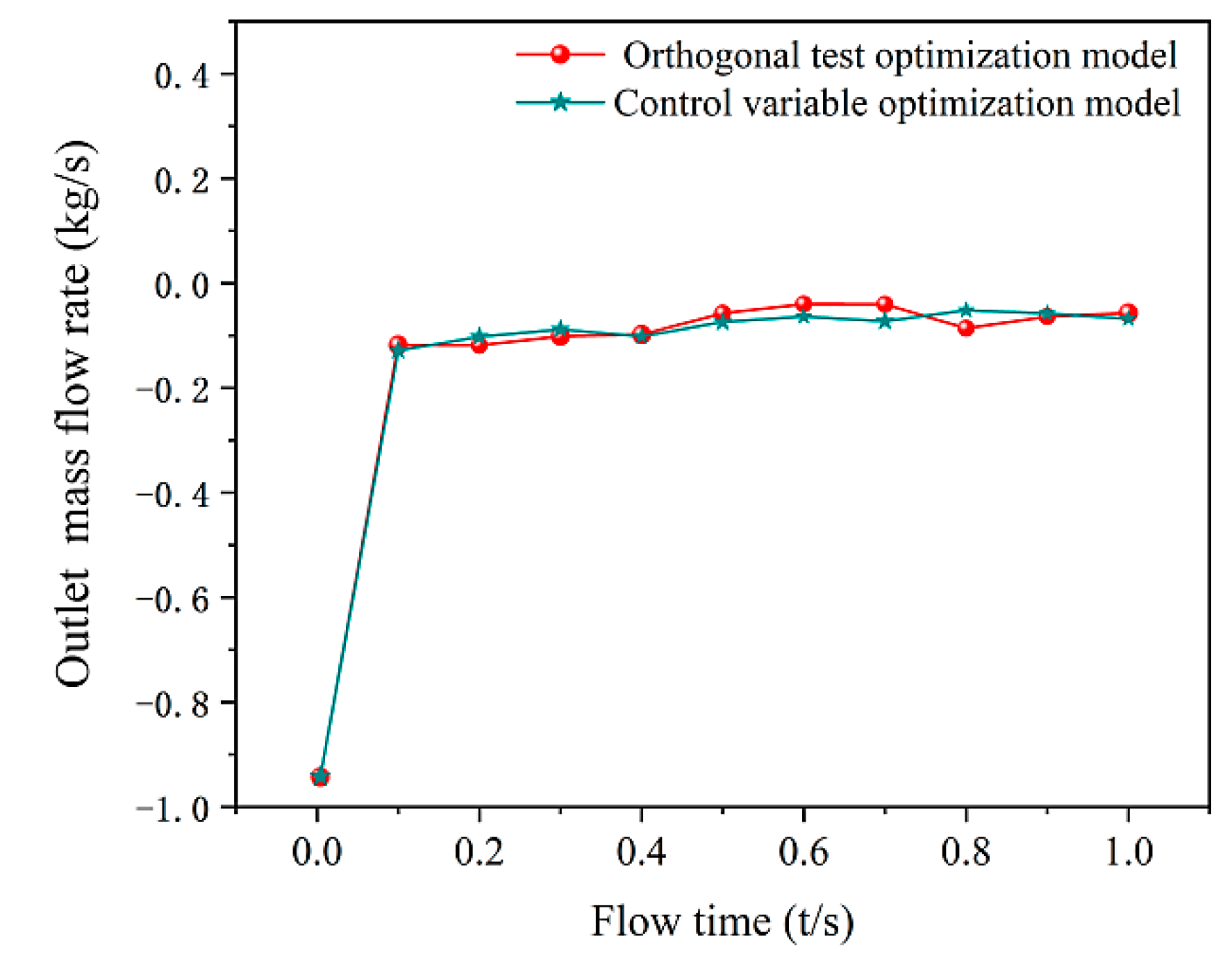
Although it is feasible to collect MR polishing fluid by air seal, the optimal collector model according to orthogonal test results still fluctuates significantly within the range of 0.4–0.8 s, and the instantaneous minimum collection efficiency is 62.4% within 1 s.
(4)
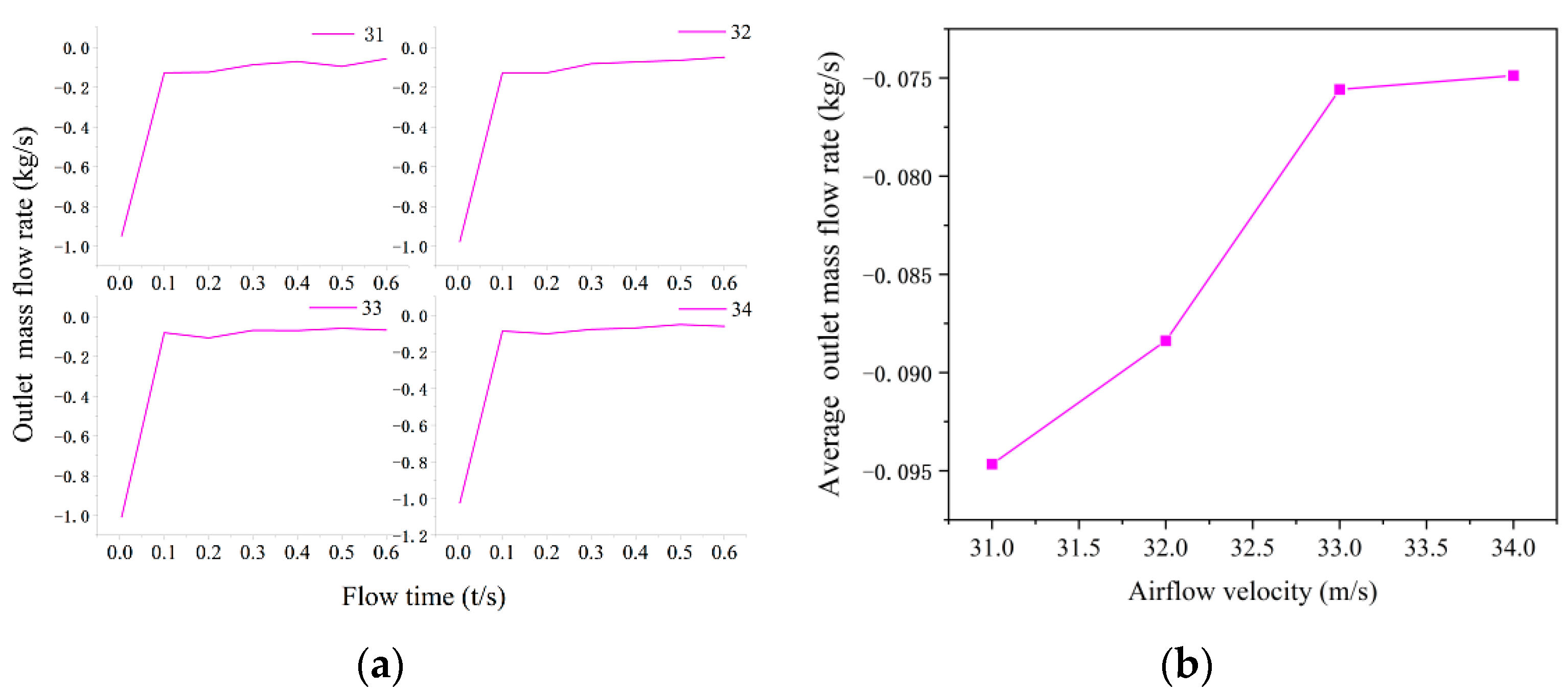
The optimal model of orthogonal experimentation was optimized by the control variable method, and it was found that the average outlet mass flow rate was the highest when the nozzle diameter and nozzle airflow velocity were 2.5 mm and 31 m/s, respectively. Excessive nozzle diameter and airflow velocity enhance the dispersion of MR polishing fluid, resulting in a decrease in mass flow rate collected by the collector.
In this study, only simulation software was used to simulate the feasibility of collecting MR polishing fluid by air seal. In future research, this collection method will be verified by experiments to explore the collection efficiency under different working conditions and compared with traditional magnetically sealed collectors.

Author Contributions

M.L. conceived and designed the analysis, collected and analyzed data, and wrote and revised the paper; G.C. conceived and designed the analysis and revised the paper; W.Z. provided guidance on the numerical simulation software; Y.P. provided the parameters required for the simulation; S.C. reviewed and validated the simulation results; J.H. provided relevant references. All authors have read and agreed to the published version of the manuscript.

Funding

This research received no external funding.

Institutional Review Board Statement

Not applicable.

Informed Consent Statement

Not applicable.

Data Availability Statement

Not applicable.

Acknowledgments

The authors thank the anonymous reviewers, who provided valuable suggestions that improved the manuscript.

Conflicts of Interest

The authors declare no conflict of interest.

References

  1. Luo, H.; Guo, M.; Yin, S.; Chen, F.; Huang, S.; Lu, A.; Guo, Y. An atomic-scale and high efficiency finishing method of zirconia ceramics by using magnetorheological finishing. Appl. Surf. Sci. 2018, 444, 569–577. [Google Scholar] [CrossRef]
  2. Jian, Y.; Tang, T.; Swain, M.V.; Wang, X.; Zhao, K. Effect of core ceramic grinding on fracture behaviour of bilayered zirconia veneering ceramic systems under two loading schemes. Dent. Mater. 2016, 32, 1453–1463. [Google Scholar] [CrossRef] [PubMed]
  3. Kang, D.; Cho, H.; Yoo, Y.; Kim, J.; Park, Y.; Moon, H. Effect of polishing method on surface roughness and bacterial adhesion of zirconia-porcelain veneer. Ceram. Int. 2017, 43, 5382–5387. [Google Scholar] [CrossRef]
  4. Vishwas, G.; Anant, K.S. Analysis of particles in magnetorheological polishing fluid for finishing of ferromagnetic cylindrical workpiece. Part. Sci. Techol. 2018, 36, 799–807. [Google Scholar]
  5. Chen, S.; Zhang, B.; Huang, J.; Yang, J. Analysis of magnetorheological fluid flow considering extrusion and wall slip. Mech. Desi. Manuf. 2022, 60, 100–103. [Google Scholar]
  6. Hao, R.S.; Li, D.C. Development Characteristics and Application Prospects of Magnetorheological Fluids. Mech. Eng. 2005, 7, 32–33. [Google Scholar]
  7. Horváth, B.; Decsi, P.; Szalai, I. Measurement of the response time of magnetorheological fluids and ferrofluids based on the magnetic susceptibility response. J. Intel. Mat. Syst. Str. 2022, 33, 918–927. [Google Scholar] [CrossRef]
  8. Ghosh, G.; Sidpara, A.; Bandyopadhyay, P.P. Review of several precision finishing processes for optics manufacturing. J. Micromanuf. 2018, 1, 170–188. [Google Scholar] [CrossRef]
  9. Tang, C.X.; Wen, S.L.; Zhang, Y.; Yan, H. Magnetorheological fluid circulation system structure under the condition of small flow rate in magnetorheological polishing. Proc. Spie. Intern. Soci. Opti. Eng. 2021, 11763, 2302–2312. [Google Scholar]
  10. Zhang, F. Research progress of magnetorheological finishing technology at CIOMP. Laser Optoelectron. Prog. 2015, 9, 92201–92202. [Google Scholar]
  11. Wang, B.; Shi, F.; Tie, G.P.; Zhang, W.L. The Cause of Ribbon Fluctuation in Magnetorheological Finishing and Its Influence on Surface Mid-Spatial Frequency Erro. Micromachines 2022, 13, 697. [Google Scholar] [CrossRef] [PubMed]
  12. Kumar, M.; Kumar, V.K.A.; Yadav, H.N.S.; Das, M. CFD analysis of MR fluid applied for finishing of gear in MRAFF process. Mater. Toda. Proc. 2021, 45, 4677–4683. [Google Scholar] [CrossRef]
  13. Luo, B.; Yan, Q.S.; Chai, J.F.; Song, W.Q.; Pan, J.S. An ultra-smooth planarization method for controlling fluid behavior in cluster magnetorheological finishing based on computational fluid dynamics. Prec. Eng. 2022, 74, 358–368. [Google Scholar] [CrossRef]
  14. Manas, D.; Jain, V.K.; Ghoshdastidar, P.S. A 2D CFD simulation of MR polishing medium in magnetic field-assisted finishing process using electromagnet. Int. J. Adv. Manuf. Techol. 2015, 76, 173–187. [Google Scholar]
  15. Prabhat, R.; Balasubramaniam, R.; Jain, V.K. Analysis of magnetorheological fluid behavior in chemo-mechanical magnetorheological finishing (CMMRF) process. Prec. Eng. 2017, 49, 122–135. [Google Scholar]
  16. Nitesh, K.D.; Dubey, N.K.; Sidpara, A. Numerical and experimental study of influence function in magnetorheological finishing of oxygen-free high conductivity (OFHC) copper. Smart Mater. Struct. 2021, 30, 015034. [Google Scholar]
  17. Yang, H.; Gu, J.H.; Huang, W.; He, J.G. Cross-experimental study on the influence mechanism of the secondary section of the polished ribbon on the pressure field creation. Manuf. Techol. Mach. Tool. 2022, 6, 18–24. [Google Scholar]
  18. Yang, H.; Ren, F.J.; Zhang, Y.F.; Huang, W.; He, J.G.; Jia, Y. Numerical analysis of formation mechanism of shear force field in the entrance zone of magnetorheological polishing. Opti. Techol. 2022, 48, 153–158. [Google Scholar]
  19. Zhang, J.J. Research on Distribution of Ultra-Precision Magnetorheological Finishing Force at Semiconductor Wafer; Beijing Jiaotong University: Beijing, China, 2020; p. 86. [Google Scholar]
  20. Gao, S. Research on Consistency of Two-Phase Flow Effect of Magnetorheological Polishing Liquid; Beijing Jiaotong University: Beijing, China, 2020; p. 92. [Google Scholar]
  21. Zhang, Z.J.; Yin, X.M.; Liu, J.G. Preparation and performance of composite coating with wear resistance on buff wheel. Corr. Prot. 2008, 7, 407–409. [Google Scholar]
  22. He, J.H. Tribological Performance of the Surface of Magnetic Rheological Polishing Wheel Treated by Microarc Oxidation; University of Electronic Science and Techolnology of China: Chengdu, China, 2016; p. 76. [Google Scholar]
  23. William, K. Multiple application of magnetorheological effect in high precision finishing. J. Intel. Mat. Syst. Struct. 2002, 13, 401–404. [Google Scholar]
  24. Dong, G.Z. Design of Small-Aperture Magnetorheological Finishing and the Device Key Technology Research; Changsha University of Science and Technology: Changsha, China, 2015; p. 76. [Google Scholar]
  25. Lu, J.Y. Research on Inverted Device for Magnetorheological Finishing; Harbin Institute of Technology: Harbin, China, 2008; p. 54. [Google Scholar]
  26. Wang, A.W. Study and Application on the Key Techniques of Magnetorheological Finishing Processing and Device; Donghua University: Shanghai, China, 2008; p. 107. [Google Scholar]
  27. Wang, D.W. A Recovery Device for Sealing Structure and Magnetorheological Polishing Liquid. CN Patent CN216151878U, 18 September 2021. [Google Scholar]
  28. Li, Y.; He, J.G.; Huang, W.; Zhang, Y.F.; Qian, L.H. Analysis of influence factors on magnetorheological polishing wheel wear. Lubr. Seal. 2019, 44, 126–131. [Google Scholar]
  29. Li, Y. Study on Wear Mechanism and Suppression Method of Magnetorheological Polishing Wheel; China Academy of Engineering Physics: Mianyang, China, 2019; p. 66. [Google Scholar]
  30. Tan, C.; Zhang, K.P. Research Advance in Granular Flow Mathematical Model; Hebei University of Science and Technology: Shijiazhuang, China, 2013; pp. 34, 293–296, 380. [Google Scholar]
  31. Zhao, B.J.; Yuan, S.Q.; Liu, H.L.; Huang, Z.F.; Ming, G. Simulation of solid-liquid two-phase turbulent flow in double-channel pump based on Mixture model. J. Agricult. Eng. 2008, 1, 7–12. [Google Scholar]
  32. Hu, H.; Da, Y.F.; Peng, X.Q. Design and research of the inverted device for magnetorheological finishing. Avia. Prec. Manufact. Techol. 2006, 6, 5–8. [Google Scholar]
  33. Dong, G.Z.; Hu, H.; Li, S.Y.; Yang, C. Design and optimization of small bore magnetorheological finishing device for permanent magnet. Nanotechol. Prec. Eng. 2015, 13, 251–257. [Google Scholar]
  34. Ma, Z.Q. Study on Preparation and Properties of Magnetorheological Polishing Fluid for Ultra Precision Polishing of Miconductor Wafer; Beijing Jiaotong University: Beijing, China, 2021; p. 85. [Google Scholar]
Figure 1. Schematic diagram of the inverted MR polishing device. (a) MR polishing schematic, (b) traditional magnetic seal collector, (c) air seal collector.
Applsci 12 07433 g001
Figure 2. Traditional collector and new collector. (a) Magnetic-seal collector, (b) scraper collector, (c) new air-seal collector.
Applsci 12 07433 g002
Figure 3. Simplified collector process.
Applsci 12 07433 g003
Figure 4. Airflow seal collection device construction.
Applsci 12 07433 g004
Figure 5. Cloud map of magnetic field distribution.
Applsci 12 07433 g005
Figure 6. Mesh and boundary conditions of the model.
Applsci 12 07433 g006
Figure 7. Model grid quality.
Applsci 12 07433 g007
Figure 8. Schematic diagram of geometric factors.
Applsci 12 07433 g008
Figure 9. Model 1 polishing fluid collection cloud diagram. (a) Front view of DM collection, (b) prone view of DM collection, (c) front view of CIP collection, (d) prone view of CIP collection, (e) front view of CeO2 collection, (f) prone view of CeO2 collection.
Applsci 12 07433 g009
Figure 10. Quadrature model flow rate.
Applsci 12 07433 g010
Figure 11. Outlet flow rate variance.
Applsci 12 07433 g011
Figure 12. Effect curve of collector outlet flow rate fluctuation value.
Applsci 12 07433 g012
Figure 13. Optimal model inlet and outlet flow.
Applsci 12 07433 g013
Figure 14. Model transient collection efficiency.
Applsci 12 07433 g014
Figure 15. Collector outlet flow rate with different nozzle diameters. (a) Outlet flow rate line chart, (b) average outlet flow rate.
Applsci 12 07433 g015
Figure 16. Collector outlet mass flow rate with different values of nozzle air velocity. (a) Outlet flow rate line chart, (b) average outlet flow rate.
Applsci 12 07433 g016
Figure 17. Comparison chart of optimal collection model traffic.
Applsci 12 07433 g017
Table 1. Parameters of the mixed phase.
ComponentDWCIPCeO2
Density (g/cm3)1.07.87.13
Viscosity (Pa·s)0.0011.72 × 10−51.72 × 10⁻⁵
Volume fraction (%)60364
Particle size (um) 33
Permeability (H/m)110001
Conductivity (S/m)5.89 × 10−8
Table 2. Factor levels.
Factor 1
φ
Factor 2
D
Factor 3
θ
Factor 4
L
Factor 5
α
Factor 6
V
Level 11 mm2.5°5 mm45°25 m/s
Level 21.5 mm8 mm90°30 m/s
Level 32 mm3.5°10 mm135°35 m/s
Table 3. Range analysis.
ItemLevelFactor 1
φ
Factor 2
D
Factor 3
θ
Factor 4
L
Factor 5
α
Factor 6
V
K-value1−0.45−0.80−0.44−0.41−0.39−0.39
2−0.58−0.47−0.53−0.54−0.56−0.28
3−0.41−0.17−0.47−0.49−0.48−0.77
Kavg value1−0.08−0.13−0.07−0.07−0.07−0.06
2−0.10−0.08−0.09−0.09−0.09−0.05
3−0.07−0.03−0.08−0.08−0.08−0.13
Best level331112
R0.030.100.010.020.030.08
Table 4. Significant variance analysis.
Source of VarianceSSDFMean Square DeviationFContribution Rate (%)
Factor 10.00320.00130.9820.067
Factor 20.03320.016412.81244.345
Factor 30.00120.00030.2352.871
Factor 40.00120.00060.4711.984
Factor 50.00220.00120.9180.309
Factor 60.02220.01128.71828.976
Error0.00650.0013//
Summation0.06817///
DF: degrees of freedom; SS: sum of squares; ‘/’: null.
Publisher’s Note: MDPI stays neutral with regard to jurisdictional claims in published maps and institutional affiliations.

