Abstract
The recommendation model based on the knowledge graph (KG) alleviates the problem of data sparsity in the recommendation to a certain extent and further improves the accuracy, diversity, and interpretability of recommendations. Therefore, the knowledge graph recommendation model has become a major research topic, and the question of how to utilize the entity and relation information fully and effectively in KG has become the focus of research. This paper proposes a knowledge graph recommendation model based on adversarial training (ATKGRM), which can dynamically and adaptively adjust the knowledge graph aggregation weight based on adversarial training to learn the features of users and items more reasonably. First, the generator adopts a novel long- and short-term interest model to obtain user features and item features and generates a high-quality set of candidate items. Then, the discriminator discriminates candidate items by comparing the user’s scores of positive items, negative items, and candidate items. Finally, experimental studies on five real-world datasets with multiple knowledge graph recommendation models and multiple adversarial training recommendation models prove the effectiveness of our model.
1. Introduction
With the development of the Internet, the amount of data is increasing exponentially. Therefore, it is difficult for users to quickly find information to meet their needs. The emergence of recommender systems has effectively alleviated this problem. However, the traditional recommendation system is seriously plagued by the problems of sparse interaction data and cold starts. Many researchers have introduced the knowledge graph (KG) [1,2] into the recommendation model to solve this dilemma. Rich semantic associations can compensate for the sparseness of user historical interaction data. Therefore, the question of how to utilize the entity and relation information fully and effectively in KGs has become the focus of these studies.
In recent years, generative adversarial networks (GANs) have developed rapidly in the field of deep learning due to their powerful ability to learn complex real data distributions [3,4]. The purpose of a GAN is to conduct an adversarial battle between the generator (G) and the discriminator (D). The generator focuses on capturing the distribution of real data, generating adversarial samples, and fooling the discriminator; at the same time, the discriminator tries to distinguish whether the input samples come from the generator or not. Therefore, we proposed a KG recommendation model based on adversarial training (ATKGRM). This method can dynamically and adaptively adjust the aggregation weight of the knowledge graph, reasonably capture the content information of items, and better mine item features. Specifically, the model has two modules: G and D. G learns the real data distribution in the training data and then generates candidate items. D compares the user’s scores on candidate items, positive items, and negative items and then identifies candidate items more accurately.
This paper makes three main contributions:
- ⬤
- In this paper, adversarial training is introduced into the KG recommendation model. Therefore, the knowledge graph aggregation weight can be dynamically and adaptively adjusted to obtain more reasonable user features and item features.
- ⬤
- The generator employs a long- and short-term interest model to discover the latent features of users and generates a high-quality set of candidate items. The discriminator uses a popularity-based sampling strategy to obtain more accurate positive items and negative items. It can more accurately identify candidate items by comparing the user’s scores of positive items, negative items, and candidate items. The generator and discriminator continuously improve their performance through adversarial training.
- ⬤
- We present a comparison with multiple knowledge graph recommendation models and multiple adversarial training recommendation models on five public datasets: MovieLens-1M, MovieLens-10M, MovieLens-20M, Book-Crossing, and Last. FM. Thus, the effectiveness of the ATKGRM proposed in this paper is verified.
2. Related Works
2.1. Collaborative Filtering Recommendation Model
Collaborative filtering (CF) is a class of methods for predicting a user’s preference or rating of an item, based on his previous preferences or ratings and decisions made by similar users. There is a dichotomy of CF methods: memory-based CF and model-based CF. Memory-based CF has faded out due to its poor performance on real-life large-scale and sparse data. Model-based CF learns a model from historical data and then uses the model to predict the preferences of users. With the recent development of deep learning, neural network based-CF, a subclass of model-based CF, has gained enormous attention.
Huang et al. proposed the CF-NADE [5] model, which shows how to adapt NADE to CF tasks, encouraging the model to share parameters between different ratings. However, all results of this work rely on explicit feedback, and explicit feedback is not always available or as common as implicit feedback in real-world recommender systems. Moreover, it cannot work on both explicit and implicit feedback, since the network structures are specially designed for one case. Zheng et al. proposed the NCAE [6] model to perform collaborative filtering, which works well for both explicit feedback and implicit feedback. NCAE can effectively capture the subtle hidden relations between interactions via a non-linear matrix factorization process. Li et al. proposed the NESVD [7] model, where a low-complexity probabilistic autoencoder neural network initializes the features of the user and item, and this work addresses the challenge of existing SVD algorithms, which do not fully utilize the data information. All the above models have cold start problems, and it is necessary to explore how to incorporate auxiliary information. In this paper, we introduce a knowledge graph to alleviate the problem of cold starts and data sparsity.
2.2. Knowledge Graph Recommendation Model
Knowledge graph (KG) models for recommendation include embedding-based models [8,9,10], path-based models [11,12], and federated learning-based models [13,14,15,16].
Embedding-based models can be roughly divided into two categories: translation distance models, such as TransE [8], TransH [9], TransR [10], and TransD [17]; and semantic matching models, such as DistMult [18], RESCAL [19], and Complex [20]. However, these models are not suitable for recommendation.
Path-based models utilize meta-paths between entities in the KG for recommendation, which improves the interpretability of recommendations. For example, PER [21] and FMG [22] represent the connectivity between users and items to be recommended by extracting meta-paths between entities in KG; however, these models deal with meta-paths in KG, relying heavily on time-consuming and labor-intensive manual design.
The federated learning-based model can be viewed as a hybrid of path-based and embedding-based models, which combines the embedding representations of entities and relations with path information in the KG during the aggregation process. Wang et al. proposed the RippleNet [23] model, in which RippleNet aggregates neighbor information by calculating the similarity between items and head entities in the relation space, thereby autonomously and iteratively following paths in the KG to expand the potential interests of users. Wang et al. proposed the KGCN [24] model, where KGCN aggregates neighbor information by computing the user’s preference for relations in the KG and uses graph convolutional networks [25,26,27] to automatically capture higher-order structural and semantic information. He et al. proposed the KGAT [28] model. KGAT aggregates neighbor information by computing the distances between head and tail entities in relational space and uses the idea of embedding propagation to model higher-order representations of users and items. The KGCN only considers the user’s preference for relations when aggregating neighbor information. This paper not only uses the user’s information but also comprehensively considers the relation and tail entity information, which has better interpretability. Dong et al. proposed HAGERec [29], which exploits a hierarchical attention graph convolutional network to process KG and explores users’ latent preferences from the KG’s high-order connection structure. Wang et al. proposed the CKAN [30] model, which uses a novel collaborative knowledge-aware attention to process KG and collaborative filtering information simultaneously.
2.3. Adversarial Training in Recommendation Systems
Adversarial training has been widely studied due to its powerful ability to learn complex real data distributions. In 2014, Goodfellow et al. proposed the generative adversarial network (GAN) [31]. GANs are gradually becoming a research hotspot, and GANs are superior in many tasks, such as image generation [32], image understanding [3], and sequence generation [4]. With the development of GANs, it has become an inevitable trend to apply them to recommender systems. Wang et al. proposed the IRGAN [33] model, in which the generative model selects indistinguishable samples from the sample set and inputs them to the discriminant model for discrimination, which is mainly used in information retrieval. The generator generates a discrete item index, which may lead to two contradictory label values for one index, and it will confuse the discriminator. The discriminator will send the wrong information to the generator, which degrades the performance of both. The competition between them does not help to fully exploit the advantages of adversarial networks. Chae et al. proposed the CFGAN [34] model, whose generator generates continuous vectors instead of a discrete item index, successfully solving the above problems. To provide recommendations for new users or items, Takato et al. proposed the GCGAN [35] model, which combines GAN and graph convolution and can effectively learn domain information by propagating feature values through a graph structure. It was confirmed that the GCGAN had better performance than the conventional CFGAN. It is worth noting that the positive and negative items in the above methods are randomly sampled, so their quality cannot be guaranteed. Implicit data are inherently noisy; for example, the interactive item may be purchased by the user out of herd mentality and may not be the item that the user truly seeks. Therefore, it is necessary to adjust the sampling model to minimize the misleading nature of the discriminator caused by the randomness of sampling. In this paper, the popularity sampling strategy is used in the discriminator to obtain more accurate positive and negative items to select candidate items.
3. Our Model
This section proposes a knowledge graph recommendation model based on adversarial training (ATKGRM). In this section, we first give an overview of the ATKGRM and then introduce the generator, discriminator, and adversarial training process in the model in detail.
3.1. Model Overview
The ATKGRM consists of a generator and a discriminator. In the generator, a new long- and short-term interest model is adopted to model user features and item features and generate high-quality candidate item sets. In the discriminator, to better discriminate candidate items, we use the popularity-based sampling strategy accurately to obtain the user’s positive items and negative items and compare the user’s scores on the positive items, candidate items, and negative items to identify candidate items more accurately. The performance of the overall adversarial model is improved by a high-quality generator and a high-quality discriminator.
As shown in Figure 1, for generator G, in order to better mine user features and generate candidate items for users, user features are divided into two sections. To better mine item features, it is critical to reasonably capture the item information in the knowledge graph. First, an item-centric knowledge graph is constructed at the item embedding layer to obtain the vector representations of historical items and target items. Then, in the user modeling layer, the user representation consists of the user short-term feature and the user long-term feature . It filters the L historical items of the user’s recent interaction, integrating the corresponding location coding information and inputting it into the self-attention mechanism to obtain the potential relation between the user’s recent interaction items. The output result takes the mean operation to obtain the user’s short-term interest. Location coding is added to obtain the effect of the item’s time information. The long-term interests of users can be obtained through training based on all historical interaction items. The user representation is obtained by combining and through a multilayer perceptron (MLP). Finally, the user score of the target item (k = 1, 2, …, K) is predicted by the inner product, and the high-quality candidate item set is obtained by the sorting score (Rank).
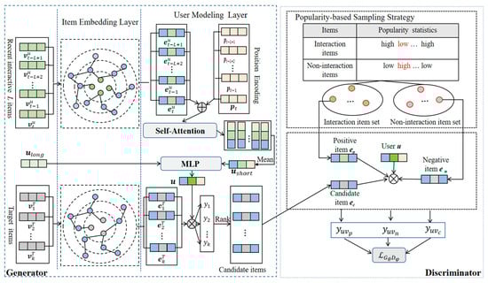
Figure 1.
Illustration of the proposed ATKGRM model.
For discriminator D, first, to better identify the candidate items generated by generator G, the popularity-based sampling strategy is used to accurately obtain the positive items and negative items from the interaction item sets and the noninteraction item sets. Then, the inner product of the user representation and the positive item vector , the negative item vector , and the candidate item vector are taken to obtain the scores , , and . Finally, the scores are input into the adversarial training loss function.
3.2. The Generator
3.2.1. Item Embedding Layer
In the item embedding layer of the generator, we need to obtain representations of recent interactive items and target items. Figure 2 shows the knowledge graph information aggregation process.
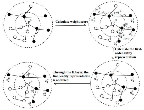
Figure 2.
The process of knowledge graph information aggregation.
As shown in Figure 2, the KG is built with the item as the central node, and each item can build a KG. It can be represented by triples (h, r, t). Here, h ∈ E, r ∈ R, and t ∈ E represent the head entity, relation, and tail entity, respectively. E and R are the entity set and the relation set, respectively. The first graph in Figure 2 builds a knowledge graph with the item as the center, and the second graph is obtained by randomly sampling the number of nodes and calculating the weight score of the knowledge graph preference attention. Through Formula (5), the first-order entity representation in the third figure can be obtained, and the above operations can be repeated to obtain the h-order entity representation . The following mainly introduces the one-layer structure and expands to the multilayer structure. For an item , denotes the set of one-hop neighbors directly connected to , and represents the relation between entities and . The weight score is calculated by using the following knowledge graph preference attention formula:
where , , and are the representations of the users and the relations between entities and tail entities, respectively, σ is a nonlinear function, d is the dimension, and and are weights and offsets. indicates the user preference for the comprehensive consideration of relations and entities. The parameters W1 and b1 can be adjusted according to the feedback of the discriminator, thereby adaptively adjusting the aggregation weight of the neighbor information.
By calculating the linear combination of item ’s neighbors, the neighbor information vector of item is obtained to represent
where denotes the representation of the item neighbor entity. The following formula is the normalization of the weight score:
We sum the representation of the item and its neighborhood representation to obtain the item representation fused with neighborhood information:
where and are weights and biases, respectively. σ is a nonlinear function.
The KG is a multilayer structure that can obtain low-order entity information at the low level and mine high-order entity information at the high level. The h-order vector of an entity is the aggregation of entity information between the entity itself and its h-hop neighborhood. We use the following Formula (6) to calculate the h-order vector representation of the item, where denotes the final item representation.
where denotes the representation of the item aggregated H-1 hop neighborhood entity. denotes the representation of H-hop neighborhood information. and are weight and biases, respectively, and σ is a nonlinear function.
3.2.2. User Modeling Layer
Considering the actual situation, the user’s long-term interest represents the hobby formed by the user over a long time. The user’s short-term interest is the user’s recent interests and hobbies, which will change over time. L recent interactive items and the corresponding position codes are added in the form of vectors. The obtained vector is input into the self-attention mechanism to obtain the potential connection between the user’s recent interaction items. The output results use the mean operation to obtain and train it based on all historical items interacted with by the user. The user’s long-term interest representations and are united by a multilayer perceptron (MLP) to obtain the user’s representation u.
Specifically, there are M users and N items in the recommendation model, which are recorded as and , respectively, with representing the embedded representation of the entire item set. For user u, we select L historical items (from item t − L + 1 to item t) that the user has interacted with recently within the time step t; then, is used to represent the initialized embedding representation of the L item sequence chosen in the set, as shown in Equation (7):
where t is the time step, L is the number of recently interacted items, and d is the dimension of the matrix.
As shown in Formula (8), is added into the item embedding layer to obtain the user’s recent interactive item representation containing knowledge graph information.
As shown in (9), to maintain the time sequence of the user’s recent interactive items, the item relative position coding information , is integrated into the representation of the item.
As shown below, the position coding function consists of sin and cos signals, where t is the time step and i is the embedded dimension.
where t represents the t-th row in the matrix. i represents the i-th column in the matrix. and represent the sine function and cosine function, respectively.
By inputting the fused information () into the self-attention mechanism, the potential relation between the recent user’s interactive items is calculated. The formula is as follows:
where denotes the weight matrix of the query and key, respectively. denotes the L × L matrix, which stands for the similarity between L items. d denotes the embedded dimension. is used to scale the similarity value. ReLU is the activation function of the nonlinear layer. The scaling factor can reduce the influence of the smallest gradient. The mask operation (masking the diagonal with a value of 0) before the normalized exponential function (softmax) is applied to avoid high matching scores between and .
We use the following formula to calculate the user’s short-term interest expression .
where L represents the number of items recently interacted with by the user, is the similarity matrix, and represents the representation of the user’s recent interaction items containing knowledge graph information.
According to the training of all historical items of user interaction, is obtained. and are input into the MLP together. A hidden layer is taken to completely obtain the user preference, which is recorded as .
where and are the weight and bias of the MLP, respectively.
3.2.3. Generate Candidate Items
We obtain the probability of interaction through the inner product. For a user, we sort all the probability values calculated by Formula (17) and take the top-N recommendation to the user.
To generate high-quality candidate items for adversarial training, the ATKGRM needs to pretrain the generator in advance. The loss function of the pretraining generator is:
where represents the cross-entropy loss function, =1 denotes the interaction between the user and positive item, =0 indicates that the user does not interact with the negative item, is the regularization coefficient, and is a parameter.
3.3. The Discriminator
To better identify the candidate items generated by generator G, we use a popularity-based sampling strategy to accurately obtain the user’s positive and negative items from the interaction item sets and the noninteraction item sets. For the selection of positive items, the user-interacted items have high popularity, which does not fully verify that the user likes the item. For example, due to herd mentality, if the user-interacted item has lower popularity, it indicates that users are truly interested in the item to a large extent. Similarly, for the selection of negative items, we choose items with high popularity from the noninteraction item set as negative items.
The main process of the strategy based on popularity sampling is as follows. First, we use the number of users who have interacted with the item to calculate the popularity of the item. The item popularity is calculated by Formula (19). Then, the average popularity of all items is calculated as the middle popularity (middle) by Formula (20). We define popularity above middle as high popularity (high) and popularity below it as low popularity (low). Therefore, items can be divided into high-popularity items and low-popularity items. Finally, the items with low popularity are randomly sampled from the interaction item set as the sampled positive items, and the items with high popularity are randomly sampled from the noninteraction item set as the sampled negative items.
where is the number of users interacting with the j-th item, j is the number of items, and is the popularity of the j-th item.
At present, adversarial training is applied to recommendation models, and most of them compare the user’s scores on positive items and candidate items through the discriminator to identify the candidate items, but there is no reasonable analysis of the candidate items. The user’s scores on the candidate items should be in between the user’s scores for positive items and negative items. Therefore, this paper proposes to identify candidate items in the discriminator by comparing the user’s scores of positive items, negative items, and candidate items. The main idea is that the user’s scores on candidate items will not be higher than the user’s scores on high-quality positive items, and the user’s scores on candidate items will not be lower than the user’s scores on high-quality negative items.
The pretraining of discriminator D uses the Bayesian Personalized Ranking (BPR) loss function. The smaller the overall loss function, the better. The formula for the pretrained discriminator is shown in Equation (21).
where is the sigmoid function, is the model parameter, () can be understood as , , the items interacted with by users are 1, and the items not interacted with by users are 0. indicates the user score on item I, and represents the user score on item j. By minimizing the loss function, a better BPR model can be trained.
3.4. Adversarial Training
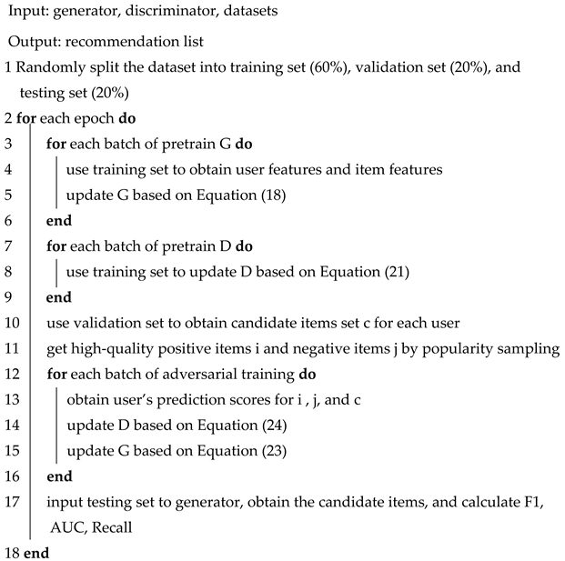
As shown in Algorithm 1, the adversarial training process of the ATKGRM model mainly includes three parts: the G pretraining, the pretraining of D, and the adversarial training. The purpose of the pretraining generator is to create new candidate items for users through trainable generative models. The purpose of the pretraining discriminator is to identify candidate items through a trainable discriminator. The generator generates candidate items that appear similar to real samples, and the discriminator distinguishes candidate items from real samples. Through the continuous confrontation between the generator and discriminator, the real data distribution in the training data is learned.
In the stage of training generator G, the user scores of positive items and candidate items are input into the objective function of the generator’s adversarial training. The loss function of generator adversarial training is as follows:
where is the prediction score of u on , and is the prediction score of u on . is the generator parameter. To make the result generated by closer to the positive item, the goal is to narrow the gap between and . In other words, needs to be maximized.
In this paper, the policy gradient method based on reinforcement learning needs to be used to approximate the discrete solution, and the actual estimated probability of the discriminator is regarded as the actual reward and used to further optimize the generator. The objective function of the optimized generator adversarial training is shown in Equation (23).
where k is the size of the list of candidate items. represents user u’s predicted score for negative example item .
In the stage of training the discriminator, the user’s scores on the positive items, negative items, and candidate items are input into the objective function of the discriminator adversarial training, to obtain more reasonable candidate items. The objective function for the adversarial training of the discriminator is shown in Equation (24).
where , represent the accurate positive items and negative items obtained from popularity sampling, and represents the high-quality candidate items obtained from the candidate item set. φ is the discriminator parameter. The first part in the formula comes from the candidate items and the positive items. We hope to widen the gap between the user’s score of the positive item and the user’s score of the generated candidate item. The second part in the formula comes from the candidate item generated by the generator G and the real negative item. We hope to widen the gap between the user’s score of the negative item and the user’s score of the generated candidate item. The goal is to minimize the discriminator training loss function.
| Algorithm 1 ATKGRM Adversarial Training Algorithm |
 |
4. Experiments
In this section, the effectiveness of the ATKGRM is verified by analyzing three sets of experiments on the collaborative filtering recommendation model, the knowledge graph recommendation model, and the adversarial training recommendation model. The importance of the adversarial training module and the popularity-based sampling strategy module is verified by eliminating these two modules for ablation experiments. At the same time, by analyzing the selection of the value of the user’s recent interactive items L and the selection of the value of the iterative layer H in the knowledge graph, two sets of experiments are used to prove the effect of the changes in the mode parameters. Furthermore, by comparing the complexity of the algorithm, the scalability of the model on large-scale data is verified.
4.1. Experimental Settings
4.1.1. Dataset
We test the performance of our model, ATKGRM, on five real-world benchmarks: MovieLens-1M1, MovieLens-10M2, MovieLens-20M3, Book-Crossing4, and Last. FM5. Among them, the MovieLens-1M, MovieLens-10M, and MovieLens-20M datasets are benchmark movie datasets with different scales, and they are widely used in knowledge graph recommendation; Book-Crossing contains 1 million ratings of books in the Book-Crossing community; Last. FM is a music listening dataset collected from the Last.fm online music system. The specific statistical results of the datasets can be seen in Table 1.

Table 1.
Statistics of the datasets.
4.1.2. Evaluation Metrics
To measure the performance of the ATKGRM, this section uses the values of RMSE, F1, area under curve (AUC), and recall as evaluation indicators.
Prediction error is measured by Root Mean Squared Error (RMSE). The formula for RMSE is shown in (25).
Recall is the ratio of the intersection of the item set recommended by the model for the user and the item set that the user actually likes; it indicates the retrieval rate of the recommended model. The larger the recall value is, the higher the retrieval rate of the recommendation model. The formula for Recall is shown in (26).
where Rec(u) is the candidate item set for user u, and Fav(u) is the set of items that user u actually likes.
The F1 value is shown in Formula (27).
where precision and recall are the accuracy rate and the recall rate, respectively. The F1 value comprehensively considers the two indicators of precision and recall.
The AUC is used to evaluate the performance of recommender systems to distinguish between user likes and dislikes. Each time the recommendation system compares the score of the item that the user likes and the item that the user does not like, is the total number of comparisons. is the number of times that the user’s scores for their favorite items are greater than the user’s scores for their disliked items, and is the number of times that the user’s scores for their favorite items are equal to the user’s scores for their disliked items. The calculation of AUC is shown in Formula (28).
4.1.3. Parameter Settings
The parameter settings in the experiment are shown in Table 2. N is the number of samples of neighbor nodes in KG, d denotes the vector dimension, H is the number of iteration layers of KG, L is the number of recent user interaction items, is the regularization coefficient, batch is the batch size, and lr is the learning rate. In the experiment, each dataset is randomly divided into a training set, validation set, and testing set, and the division ratio is 6:2:2.
Table 2.
Experimental parameter setting.
4.2. Performance Comparison
4.2.1. Performance Comparison with the Collaborative Filtering Model
The ATKGRM-KG and three baseline collaborative filtering recommendation models are compared on MovieLens-1M and MovieLens-10M. Because these three models do not use knowledge graph information, we used ATKGRM-KG, which removed the process of aggregating knowledge graph information from ATKGRM, for a more accurate comparison. The comparison of the baseline models is shown in Table 3.
Table 3.
RMSE of different models on MovieLens-1M and MovieLens-10M.
Three baseline collaborative filtering recommendation models are introduced below:
- ⬤
- CF-NADE [5] shows how to adapt NADE to CF tasks, encouraging the model to share parameters between different ratings;
- ⬤
- NCAE [6] can effectively capture the subtle hidden relationships between interactions via a nonlinear matrix factorization process;
- ⬤
- NESVD [7] proposes a general neural embedding initialization framework, where a low-complexity probabilistic autoencoder neural network initializes the features of the user and item.
The results can be seen in Table 3. It is worth noting that the underscore represents no corresponding data. The ATKGRM-KG model has superior performance. Specifically, on the MovieLens-1M dataset, compared with the optimal baseline collaborative filtering recommendation model NESVD and CF-NADE, the RMSE of ATKGRM-KG is reduced by 38.1% and 38.4%, respectively. On the MovieLens-10M dataset, compared with NESVD, CF-NADE, and NCAE, the RMSE of ATKGRM-KG is reduced by 42.1%, 42.8%, and 42.5%. ATKGRM-KG is better than NESVD, CF-NADE, and NCAE, which can show the advantages of adversarial training. The purpose of GAN is to conduct an adversarial battle between the generator and the discriminator and it is an effective way to alleviate data noise.
4.2.2. Performance Comparison of the Knowledge Graph Recommendation Model
The ATKGRM is compared with seven baseline knowledge graph recommendation models on the same three public datasets.
The seven baselines knowledge graph recommendation models are introduced below:
- ⬤
- CKE [36] uses TransE [8] to preprocess entity and relationship information in KG to model user and item features;
- ⬤
- PER [21] extracts the information of meta-paths in a knowledge graph to show the connectivity between items and users on diverse types of relationship paths;
- ⬤
- RippleNet [23] uses multi-hop neighborhood information to expand a user’s potential interests by iteratively and autonomously following the links in KG;
- ⬤
- KGCN [24] uses a graph convolution network to automatically obtain semantic information and a high-order structure by sampling definite neighbors as the receptive field of candidate items;
- ⬤
- KGAT [28] combines a user–item interaction graph with KG as a collaborative knowledge graph; in communication, an attention module is used to differentiate the significance of neighborhood entities in a collaborative knowledge graph;
- ⬤
- HAGERec [29] uses the convolution network of a hierarchical attention graph to process KGs and explore the potential preferences of users; to fully use semantic information, a two-way information dissemination strategy is used to obtain the vector of items and users;
- ⬤
- CKAN [30] uses the cooperative knowledge perception attention module to differentiate the contributions of diverse neighborhood entities in processing KG and collaborative information.
From Table 4 (or Figure 3), the AUC of ATKGRM in MovieLens-20M, Book-Crossing and Last.FM is increased by 0.4%, 2.5%, and 2.0%, respectively, and the F1 increases by 2.3%, 3.1%, and 0.5%, respectively.
Table 4.
Comparison results of knowledge graph recommendation models.
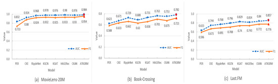
Figure 3.
Comparison results of knowledge graph recommendation models. (On three different datasets).
ATKGRM shows reliable performance. It is almost close to KGAT and HAGERec with strong performance, and it obtains the best performance in the value of individual K.
The experimental results of path-based PER are poor because PER needs to find the meta-path between users and items to be recommended, but it is difficult to obtain the best scheme for the design of the meta-path. The experimental results based on the embedded CKE model are poor because TransE may not fully use KG information. Compared with the above two methods, RippleNet, KGCN, KGAT, HAGERec, and CKAN show satisfactory performance. RippleNet independently and iteratively expands the user’s potential interests along the path in the knowledge graph but may not observe the graph information of recommended items. KGCN obtains the item representations through the graph convolution network, but KGCN does not effectively use the user’s historical items to mine the user’s potential interests. HAGERec and CKAN are superior to KGAT because HAGERec can automatically capture the representations of users and items through a two-way information dissemination strategy and filter out some noise by relying on an aggregation strategy with good interpretability. CKAN processes collaborative filtering information and knowledge graph information separately, which can effectively solve the data noise in KG and achieve satisfactory results. The ATKGRM comprehensively analyzes and and combines them to obtain the features of users. The model introduces the idea of adversarial training into the recommendation model to dynamically and adaptively adjust the aggregation weight of the knowledge graph so that it can learn the user feature and the item feature more reasonably.
4.2.3. Performance Comparison of Adversarial Training Recommendation Models
The ATKGRM and three baseline adversarial training recommendation models proposed in this paper are implemented in MovieLens-1M and Last. FM. The comparison of the baseline models is shown in Table 5.
Table 5.
Comparison results of adversarial training models.
Three types of adversarial training recommendation models are introduced below.
- ⬤
- IRGAN [33] is a pioneer in the field of recommendation using adversarial training. The discriminator in the IRGAN is used to distinguish whether the items from the generator conform to the user’s real preference distribution.
- ⬤
- CFGAN [34] is the first model to use a generator to generate a continuous vector instead of a discrete item index.
- ⬤
- GCGAN [35] combines GAN and graph convolution and can effectively learn the main information by propagating feature values through a graph structure.
By analyzing the comparison in Table 5 (or Figure 4), we can conclude that on the MovieLens-1M dataset, compared with the optimal baseline adversarial training recommendation model CFGAN, the Recall@5 and the Recall@20 of ATKGRM are increased by 2.5% and 7.2%, respectively. On the Last. FM dataset, compared with the baseline adversarial training recommendation model GCGAN, the Recall@10 of ATKGRM is increased by 11.9%. Moreover, compared with the model GCGAN, the Recall@20 of ATKGRM is increased by 11.7%. It is worth noting that we removed the user and item domain information in the model GCGAN for more accurate comparison. Among them, ATKGRM-KG means that the knowledge graph information is eliminated based on ATKGRM. ATKGRM-KG is better than IRGAN, CFGAN, and RSGAN, which can show the advantages of this adversarial training model, and ATKGRM is better than AKTGRM-KG, which can show the advantages of using a knowledge graph.
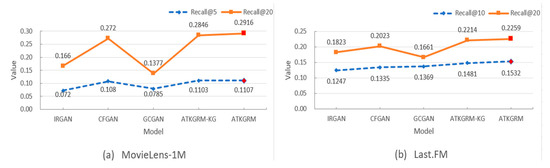
Figure 4.
Comparison results of adversarial training recommendation models. (On two different datasets).
4.2.4. Ablation Experiment
To prove the significance of introducing a generative adversarial network and popularity-based sampling strategy into the model in improving the accuracy of the model, the ablation experiment is conducted by removing the adversarial training part of the model and removing the popularity-based sampling strategy part of the model. ATKGRM-AT denotes the removal of the adversarial training part, and ATKGRM-P indicates that the sampling method based on popularity is removed.
According to the analysis in Table 6, ATKGRM shows better performance than ATKGRM-AT and ATKGRM-P. It shows that adversarial training and the popularity-based sampling method are successful in improving the performance of the model.
Table 6.
Comparison of ablation experimental results of ATKGRM.
4.3. Study of ATKGRM
4.3.1. Selection of the Number of User’s Recent Interactive Items L
Since L is the number of recent interactive items of users, and the choice of L will affect the modeling of users’ short-term interests, the influence of diverse L on experimental performance can be explored. The ATKGRM is evaluated on three datasets with different L values. The results are shown in Table 7.
Table 7.
Experimental performance of ATKGRM with different L values.
As Table 7 shows, on the MovieLens-20M, the effect of the model is the best when L = 7; on Book-Crossing, the AUC of the model is the best when L = 5. When L = 5, the F1 of the model is the best; on Last. FM, the effect of the model is the best when L = 5. If L is too small, there are too few user’s history items to effectively mine the short-term interest feature of users, which makes the effect of the model poor. If L is too large, it will lead to overfitting and inaccurate features of user short-term interest.
4.3.2. Selection of Iteration Layers H in Knowledge Graph
Since H denotes the number of iteration layers in KG, the selection of H will affect the item modeling and the user preference. Therefore, the influence of diverse H on the experimental performance can be explored.
From Table 8, the effect of the model is the best when H = 2 on MovieLens-20M. For Book-Crossing, the model works best when H = 1. On Last. FM, the model will obtain the best result when H = 1. The results indicate that the increase in aggregation layers in KG may not improve the model results. With the increase in aggregation layers in KG, more irrelevant item features in KG are taken into account, which hinders the mining of user interests.
Table 8.
Experimental performance of ATKGRM with different H values.
4.4. Complexity Analysis
The computation time of the proposed ATKGRM framework is mainly determined by evaluating the objective functions L in (21), (23), and gradients against feature vectors (variables). The time complexity of negative sampling optimization algorithms is O (log W), where W is the size of vocabulary for users and items. The computational complexity of gradients ∂L/∂u, ∂L/∂i, ∂L/∂j in (21) is O (k |Ω|), where k is the dimension of the latent vector, and |Ω| is the number of users and items observed. The computational complexity of gradients ∂L/∂u and ∂L/∂vp, ∂L/∂vc, ∂L/∂vn in (23) is O (k (r + 1) |Ω|), where r is the number of negative samples per positive instance. Therefore, the overall computational complexity of T iterations is O (k (r + 1) |Ω|T + log W) for implicit feedback. On the other hand, since explicit feedback does not require negative sampling, r = 0 is used to compute explicit feedback. The overall computation time is linear with the observations of rating matrices.
Then, we carry out a performance comparison and discussion. As shown in Table 9, our method has more parameters than NESVD and KGCN, but it corresponds to the best RMSE results on both datasets. As for NESVD, it only uses interactive data, and our model uses not only interactive data but also knowledge graph information, which increases the complexity of the model in the process of knowledge graph aggregation. Compared with KGCN, we have extra MLP layers, which increases the complexity of the model. However, the overall performance of ATKGRM is better than that of the baseline model, GCGAN. To sum up, ATKGRM does have higher complexity, but our model has achieved a good result on the value of RMSE.
Table 9.
The number of parameters and the results of RMSE on different models (M denotes “million”).
The results show that our method has more parameters than NESVD and KGCN, but it corresponds to the best RMSE results on both datasets. As for NESVD, it only uses interactive data, and our method uses not only interactive data but also knowledge graph information, which increases the complexity of the model in the process of knowledge graph aggregation. Compared with KGCN, we have extra MLP layers, which increases the complexity of the model. Moreover, the overall performance of ATKGRM is better than that of the baseline model, GCGAN, and we have advantages in both the number of parameters and RMSE.
At the same time, to verify the scalability of the model ATKGRM on large-scale data, we also expand the comparison of our model to different aggregation layers (H) and training data ratios (D).
As shown in Table 10, the overall computation time is linear with the observations of rating matrices. Our proposed ATKGRM has good potential to scale to large-scale datasets. However, there is still further room to speed up the computation time.
Table 10.
Training time per epoch on MovieLens-1M (in seconds).
5. Conclusions and Future Work
Enlightened by the application of generative adversarial networks in many fields, we propose a knowledge graph recommendation model based on adversarial training (ATKGRM). It introduces the generative adversarial network into the knowledge graph recommendation model first. Through the continuous competition between the generator and the discriminator, the knowledge graph aggregation weight is dynamically and adaptively adjusted to learn the features of users and items more reasonably. Experimental results on five real datasets validate the effectiveness of the ATKGRM. However, we found that our model has further room to speed up the implementation time. Therefore, model compression is a method that should be considered. At the same time, in order to further alleviate the problem of data sparsity and obtain better results, we will also seek to introduce transfer learning in the future.
Author Contributions
Data curation, S.Z. and S.F.; writing—original draft preparation, N.Z. and S.F.; writing—review and editing, S.Z. and N.Z.; visualization, S.Z. and N.Z.; supervision, J.G.; project administration, J.L.; funding acquisition, J.G. All authors have read and agreed to the published version of the manuscript.
Funding
This research was funded by the Key Research and Development Projects in Hebei Province [No. 20310802D].
Data Availability Statement
MovieLens-1M: https://grouplens.org/datasets/movielens/1m. MovieLens-10M: https://grouplens.org/datasets/movielens/10m. MovieLens-20M: https://grouplens.org/datasets/movielens/20m. Book-Crossing: http://www2.informatik.uni-freiburg.de/cziegler/BX. Last.FM: https://grouplens.org/datasets/hetrec-2011 (accessed on 6 April 2022).
Conflicts of Interest
The authors declare no conflict of interest.
References
- Wang, X.; Wang, D.; Xu, C.; He, X.; Cao, Y.; Chua, T.S. Explainable reasoning over knowledge graphs for recommendation. In Proceedings of the AAAI Conference on Artificial Intelligence, Honolulu, HI, USA, 27 January–1 February 2019; pp. 5329–5336. [Google Scholar]
- Sang, L.; Xu, M.; Qian, S.; Wu, X. Knowledge graph enhanced neural collaborative recommendation. Expert Syst. Appl. 2021, 164, 113992. [Google Scholar] [CrossRef]
- Chen, X.; Duan, Y.; Houthooft, R.; Schulman, J.; Sutskever, I.; Abbeel, P. InfoGAN: Interpretable representation learning by information maximizing generative adversarial nets. In Proceedings of the 30th Conference on Neural Information Processing Systems, Barcelona, Spain, 1 June 2016; pp. 2172–2180. [Google Scholar]
- Bousmalis, K.; Silberman, N.; Dohan, D.; Erhan, D.; Krishnan, D. Unsupervised pixel-level domain adaptation with generative adversarial networks. In Proceedings of the 2017 IEEE Conference on Computer Vision and Pattern Recognition, Honolulu, HI, USA, 1 July 2017; pp. 95–104. [Google Scholar]
- Zheng, Y.; Tang, B.; Ding, W.; Zhou, H. A neural autoregressive approach to collaborative filtering. arXiv 2016, arXiv:1605.09477. [Google Scholar] [CrossRef]
- Li, Q.; Zheng, X.; Wu, X. Neural collaborative autoencoder. arXiv 2017, arXiv:1712.09043. [Google Scholar] [CrossRef]
- Huang, T.; Zhao, R.; Bi, L.; Zhang, D.; Lu, C. Neural embedding singular value decomposition for collaborative filtering. IEEE Trans. Neural Netw. Learn. Syst. 2021, 9, 1–9. [Google Scholar] [CrossRef] [PubMed]
- Bordes, A.; Usunier, N.; Garcia-Duran, A.; Weston, J.; Yakhnenko, O. Translating embeddings for modeling multi-relational data. In Proceedings of the Advances in Neural Information Processing Systems (NIPS 2013), Lake Tahoe, NV, USA, 8 May 2013; pp. 2787–2795. [Google Scholar]
- Wang, Z.; Zhang, J.; Feng, J.; Chen, Z. Knowledge graph embedding by translating on hyperplanes. In Proceedings of the AAAI Conference on Artificial Intelligence, Québec City, QC, Canada, 27–31 July 2014; pp. 1112–1119. [Google Scholar]
- Lin, Y.; Liu, Z.; Sun, M.; Liu, Y.; Zhu, X. Learning entity and relation embedding for knowledge graph completion. In Proceedings of the Twenty-Ninth AAAI Conference on Artificial Intelligence, Austin, TX, USA, 25–30 January 2015; pp. 2181–2187. [Google Scholar]
- Pan, H.; Qin, Z. Collaborative filtering algorithm based on knowledge graph meta-path. Mod. Comput. 2021, 27, 17–23. [Google Scholar]
- Chen, Y.; Feng, W.; Huang, M.; Feng, S. Behavior path collaborative filtering recommendation algorithm based on knowledge graph. Comput. Sci. 2021, 48, 176–183. [Google Scholar]
- Zhang, F.; Li, R.; Xu, K.; Xu, H. Similarity-Based heterogeneous graph attention network for knowledge-enhanced recommendation. In Proceedings of the International Conference on Knowledge Science 2021, Bolzano, Italy, 16–18 September 2021; pp. 488–499. [Google Scholar]
- Li, X.; Yang, X.; Yu, J.; Qian, Y.; Zheng, J. Two terminal recommendation algorithms based on knowledge graph convolution network. Comput. Sci. Explor. 2022, 16, 176–184. [Google Scholar]
- Wang, H.; Zhang, F.; Zhang, M.; Leskovec, J.; Zhao, M.; Li, W.; Wang, Z. Knowledge-aware graph neural networks with label smoothness regularization for recommender systems. In Proceedings of the 25th ACM SIGKDD International Conference on Knowledge Discovery & Data Mining, Anchorage, AK, USA, 4–8 August 2019; pp. 968–977. [Google Scholar]
- Wang, H.; Zhang, F.; Zhao, M.; Li, W.; Xie, X.; Guo, M. Multi-task feature learning for knowledge graph enhanced recommendation. In Proceedings of the World Wide Web Conference, San Francisco, CA, USA, 13–17 May 2019; pp. 2000–2010. [Google Scholar]
- Ji, G.; He, S.; Xu, L.; Liu, K.; Zhao, J. Knowledge graph embedding via dynamic mapping matrix. In Proceedings of the 53rd Annual Meeting of the Association for Computational Linguistics and the 7th International Joint Conference on Natural Language Processing, Beijing, China, 26–31 July 2015; pp. 687–696. [Google Scholar]
- Yang, B.; Yih, W.T.; He, X.; Gao, J.; Deng, L. Embedding entities and relations for learning and inference in knowledge bases. arXiv 2014, arXiv:1412.6575. [Google Scholar]
- Nickel, M.; Tresp, V.; Kriegel, H.P. A three-way model for collective learning on multi-relational data. In Proceedings of the 28th International Conference on Machine Learning, Washington, DC, USA, 28 June–2 July 2011; pp. 809–816. [Google Scholar]
- Trouillon, T.; Welbl, J.; Riedel, S.; Gaussier, É.; Bouchard, G. Complex embeddings for simple link prediction. In Proceedings of the International Conference on Machine Learning, New York, NY, USA, 19–24 June 2016; pp. 2071–2080. [Google Scholar]
- Yu, X.; Ren, X.; Sun, Y.; Gu, Q.; Sturt, B.; Khandelwal, U.; Norick, B.; Han, J. Personalized entity recommendation: A heterogeneous information network approach. In Proceedings of the 7th ACM International Conference on Web Search and Data Mining, New York, NY, USA, 24–28 February 2014; pp. 283–292. [Google Scholar]
- Zhao, H.; Yao, Q.; Li, J.; Song, Y.; Lee, D.L. Meta-graphbased recommendation fusion over heterogeneous information networks. In Proceedings of the 23rd ACM SIGKDD International Conference on Knowledge Discovery and Data Mining, Halifax, NS, Canada, 13–17 August 2017; pp. 635–644. [Google Scholar]
- Wang, H.; Zhang, F.; Wang, J.; Zhao, M.; Li, W.; Xie, X.; Guo, M. RippleNet: Propagating user preferences on the knowledge graph for recommender systems. In Proceedings of the 27th ACM International Conference on Information and Knowledge Management, Torino, Italy, 22–26 October 2018; pp. 417–426. [Google Scholar]
- Wang, H.; Zhao, M.; Xie, X.; Li, W.; Guo, M. Knowledge graph convolutional networks for recommender systems. In Proceedings of the Worldwide Web Conference, San Francisco, CA, USA, 13–17 May 2019; pp. 3307–3313. [Google Scholar]
- Gu, J.; She, S.; Fan, S.; Zhang, S. Recommendation based on convolution network of users’ long- and short-term interests and knowledge graph. Comput. Eng. Sci. 2021, 43, 511–517. [Google Scholar]
- Xu, B.; Cen, K.; Huang, J.; Shen, H.; Cheng, X. A survey of graph convolution neural networks. J. Comput. Sci. 2020, 43, 755–780. [Google Scholar]
- Choi, J.; Ko, T.; Choi, Y.; Byun, H.; Kim, C.K. Dynamic graph convolutional networks with attention mechanism for rumor detection on social media. PLoS ONE 2021, 16, e0256039. [Google Scholar]
- Wang, X.; He, X.; Cao, Y.; Liu, M.; Chua, T.S. KGAT: Knowledge graph attention network for recommendation. In Proceedings of the 25th ACM SIGKDD International Conference on Knowledge Discovery & Data Mining, Anchorage, AK, USA, 4–8 August 2019; pp. 950–958. [Google Scholar]
- Yang, Z.; Dong, S. HAGERec: Hierarchical attention graph convolutional network incorporating knowledge graph for explainable recommendation. Knowl.-Based Syst. 2020, 204, 106194. [Google Scholar] [CrossRef]
- Wang, Z.; Lin, G.; Tan, H.; Chen, Q.; Liu, X. CKAN: Collaborative knowledge-aware attentive network for recommender systems. In Proceedings of the 43rd International ACM SIGIR Conference on Research and Development in Information Retrieval, Xi’an, China, 25–30 July 2020; pp. 219–228. [Google Scholar]
- Goodfellow, I.J.; Pouget-Abadie, J.; Mirza, M.; Xu, B.; Warde-Farley, D.; Ozair, S.; Courville, A.; Bengio, Y. Generative adversarial networks. In Proceedings of the 27th International Conference on Neural Information Processing Systems, Montreal, QC, Canada, 8–13 December 2014; pp. 2672–2680. [Google Scholar]
- He, K.; Zhang, X.; Ren, S.; Sun, J. Deep residual learning for image recognition. In Proceedings of the IEEE Conference on Computer Vision and Pattern Recognition, Las Vegas, NV, USA, 26 June–1 July 2016; pp. 770–778. [Google Scholar]
- Wang, J.; Yu, L.; Zhang, W.; Gong, Y.; Xu, Y.; Wang, B.; Zhang, P.; Zhang, D. IRGAN: A minimax game for unifying generative and discriminative information retrieval models. In Proceedings of the 40th International ACM SIGIR Conference on Research and Development in Information Retrieval, Tokyo, Japan, 7–11 August 2017; pp. 515–524. [Google Scholar]
- Chae, D.; Kang, J.; Kim, S.; Lee, J. CFGAN: A generic collaborative filtering framework based on generative adversarial networks. In Proceedings of the 27th ACM International Conference on Information and Knowledge Management, Torino, Italy, 22–26 October 2018; pp. 137–146. [Google Scholar]
- Takato, S.; Shin, K.; Hajime, N. Recommendation System Based on Generative Adversarial Network with Graph Convolutional Layers. Jaciii 2021, 25, 389–396. [Google Scholar] [CrossRef]
- Zhang, F.; Yuan, N.J.; Lian, D.; Xie, X.; Ma, W.Y. Collaborative knowledge base embedding for recommender systems. In Proceedings of the 22nd ACM SIGKDD International Conference on Knowledge Discovery and Data Mining, San Francisco, CA, USA, 13–17 August 2016; pp. 353–362. [Google Scholar]
Publisher’s Note: MDPI stays neutral with regard to jurisdictional claims in published maps and institutional affiliations. |
© 2022 by the authors. Licensee MDPI, Basel, Switzerland. This article is an open access article distributed under the terms and conditions of the Creative Commons Attribution (CC BY) license (https://creativecommons.org/licenses/by/4.0/).