Abstract
Seismic temporal properties constitute a fundamental component in developing probabilistic models for earthquake occurrence in a specific area. Earthquake occurrence is neither periodic nor completely random but often accrues into bursts in both short- and long-term time scales, and involves a complex summation of triggered and independent events (ΔT). This behavior underlines the impact of the correlations on many potential applications such as the stochastic point process for the earthquake interevent times. In this respect, we intend firstly to determine the appropriate magnitude thresholds, Mthr, indicating the temporal crossover between correlated and statistically independent earthquakes in each 1 of the 10 distinctive sub-areas of the Aegean region. The second goal is the investigation of the statistical distribution that optimally fits the interevent times’ data for earthquakes with M Mthr after evaluating the Gamma, Weibull, Lognormal and Exponential distributions performance. Results concerning the correlations analysis evidenced that the temporal crossover of the earthquake interevent time data ranges from Mthr 4.7 up to Mthr 5.1 among the 10 sub-areas. The distribution fitting and comparison reveals that the Gamma distribution outperforms the other three distributions for all the data sets. This finding indicates a burst or clustering behavior in the earthquake interevent times, in which each earthquake occurrence depends upon only the occurrence time of the last one and not from the full seismic history.
1. Introduction
The study of temporal properties of earthquakes contributes to analyzing the seismicity of a specific region in order to develop earthquake occurrence models. Earthquake occurrence is neither periodic nor completely random but often is clustered in both short- and long-term time scales [1,2] represented by a complex summation of triggered (e.g., aftershocks of a strong earthquake or swarm-like excitations) and independently distributed (spontaneous) events.
As a complex process, seismogenesis is characterized by scaling behavior [3], which is described by well-known empirical laws concerning the earthquake’s magnitude distribution (the Gutenberg–Richter Law; [4]) and the aftershock’s decay rate (the Omori Law; [5]). Focusing on the earthquake interevent time (ΔT), Bak et al. [6] stated that seismicity follows a universal scaling law, independently of the magnitude cut-off and the length of its spatial distribution. Corral [7,8] further studied this result and suggested that ΔT is optimally described by the generalized Gamma distribution.
Several studies (e.g., [9,10], among others) questioned these findings and concluded that ΔT distribution is deviated from universality. For example, Touati et al. [11] examined both real and synthetic ΔT and showed that a short ΔT between consecutive earthquakes deviated from the unified scaling behavior as a result of the interaction between the triggered and spontaneous earthquakes. They concluded that the distribution of ΔT is bimodal in a way that the correlated and independent earthquakes are following the Gamma distribution and exponential decay, respectively. In order to overcome these departures, Godano [12] proposed a new expression of the ΔT distribution, based on the Gamma distribution and included an additional parameter in its equation.
The latter conclusions underline the impact of the correlations among ΔT, not only in terms of short-term clustering as the epidemic-type models (e.g., ETAS model; [13]) assume but in a more general way. This issue is becoming the main objective of several studies over the years. For instance, Livina et al. [14] have investigated ΔT data sets of six different earthquake catalogs worldwide with various magnitude thresholds and found that they are correlated, exhibiting behavior in which short ΔT intervals are followed by short intervals and long ΔT intervals are followed by large intervals. Applications of Detrended Fluctuations Analysis (DFA) and conditional probability methods in different study areas such as Northern and Southern California [15], Italy and Israel [16,17] concluded similar results. Especially for Greece, Gkarlaouni et al. [18] applied DFA techniques for studying the memory of ΔT for two distinctive fault zones of various magnitude thresholds, namely Mthr 1.7, Mthr 2.3, Mthr 4.0 and Mthr 6.0, and for the periods 2008–2014, 2008–2014, 1981–2014 and 1700–2014, respectively. They found that the ΔT of small to moderate earthquakes exhibits strong long-range correlations whereas the ΔT data sets of large earthquakes (M 6.0) could be considered statistically independent. Parson and Geist [19] found that the ΔT of global earthquakes (M~8) that occurred between 1900 and 2011, which might be considered rare events, are characterized by a lack of memory and can be described by a Poisson process.
Given the aforementioned findings, the detection of any correlations between ΔT or the existence of memory among them is an important characteristic of their temporal behavior. The investigation of the possible influence of the different magnitude thresholds above which the samples of ΔT can be considered as statistically independent, or in other words the possibility of a crossover regime in magnitudes in which the respective ΔT change their temporal behavior from correlated to uncorrelated, is important information with many potential uses. For example, it is useful for the selection of adequate earthquake data sets for stochastic point processes modeling. For such applications, four characteristics must be qualified: (1) The numbers of events occurring in two different time intervals are mutually independent (thus the aforementioned threshold Mthr has to be detected); (2) The probability distribution of the number of events within a specific time interval depends only on the length of the interval; (3) Two or more events occur simultaneously; and (4) especially for renewal models, the occurrence of the next event depends only on the time elapsed from the last event and not on the full history [20].
The main objectives of the current study are two. Firstly, the identification of the possible correlations between ΔT in earthquake data sets with different magnitude thresholds (Mthr). This concerns moderate to large earthquake (4.1 Mw < 5.2) time intervals in 10 distinctive sub-areas of the Greek territory, and the detection of possible Mthr which designates the temporal crossover between correlated and statistically independent earthquakes. Both procedures are implemented via the application of time series analysis tools, which are widely used in seismicity studies (e.g., [21]). Specifically, in the current study, the Autocorrelation and Partial Autocorrelation Functions along with the Ljung–Box Q-test are applied. For further investigation of the memory of the ΔT data sets, Detrended Fluctuations Analysis is also applied. The second goal is seeking the statistical distribution that optimally fits the ΔT data sets for each sub-area for earthquakes with M Mthr which emerge from the application of the previous methodology. For this purpose, we tested four statistical distributions (Weibull, Lognormal, Gamma and Exponential) that are the most commonly used in investigations of earthquake ΔT data sets for the identification of the best-performing distribution.
2. Tectonic Setting
The Aegean region exhibits seismotectonic complexity, with the dominance of the subduction of the Eastern Mediterranean oceanic lithosphere beneath the Eurasian continental lithospheric plate in the southern Aegean Sea. This process forms the Hellenic Arc and its extensional back arc Aegean area [22] due to the slab roll back [23]. The Hellenic Arc is bounded to its northwestern edge by the right-lateral Kefalonia Transform Fault Zone (KTFZ) and to its southeastern edge by the left-lateral Rhoades Transform Fault (RTF). To the north of KTFZ, the continental collision of the Adriatic microplate and the Eurasia plate takes place, resulting in a compressional seismic zone running parallel both onshore and offshore to the western coastal areas of Greece and Albania. The westward motion of Anatolia as a rigid block results in the formation of the right lateral North Anatolian Fault Zone (NAFZ) extending through the Marmara Sea into the northern Aegean Sea along the North Aegean Trough (NAT), which is the boundary between the Eurasian plate and the Aegean microplate [24] (Figure 1).
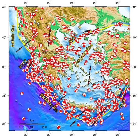
Figure 1.
The major active boundaries (solid yellow lines) and their relative motions (red arrows) in the broader Aegean Sea area, along with the available focal mechanisms of earthquakes that occurred since 1976 as derived from the Global CMT database (Available online: www.globalcmt.org (last accessed on 30 April 2022)). Fault plane solutions are shown as equal area lower hemisphere projection (compressional quadrants are depicted in red).
The available focal mechanisms of the Global Centroid Moment Tensor (Global CMT; Available online: www.globalcmt.org (accessed on 30 April 2022)) since 1976 highlighted that the vast amount of seismicity is associated with the above-mentioned and fast deformed active boundaries (Figure 1). Specifically, it is derived that the majority of the thrust fault plane solutions (fps) are concentrated in the proximity of continental collision of the Adriatic microplate and Eurasia in northwest Greece and along the Hellenic Subduction Zone active boundaries. The right lateral KTFZ and ΝATFZ are related to strike-slip fault plane solutions, and to a lesser extent in the southeastern Aegean area, where the left-lateral Rhoades Transform Fault is activated. Fast extension in N–S direction dominates in the back arc area, along with an E–W extension in the transition zone running parallel to both continental collision and oceanic subduction.
The spatial extension of the active boundaries, along with the available fault plane solutions allow the definition of seismic zones with distinctive seismotectonic properties in the study area, and then the detection of the appropriate Mthr above which the temporal crossover between correlated and statistically independent earthquakes is seeking. The 10 sub-areas that are defined, based on the aforementioned criteria, are shown in the map of Figure 2 (red polygons), along with the Mw 4.1 crustal (h 40 km) seismicity covering the time period 1975–2021. The compressional stress field of western Greece and Albania constitutes the sub-area 1, in which seismicity is concentrated along the main low angle thrust faulting structures with an NW–SE strike parallel to the coast [24] and the corresponding P-axes to be generally oriented perpendicular to the collision front (Figure 1). The dextral strike-slip KTFZ is the sub-area 2. KTFZ is a well-defined fault zone characterized by right-lateral faulting with a considerable thrust component [25]. It consists of the most active fault zone in Greece with the frequent occurrence of large (Mw ) earthquakes.
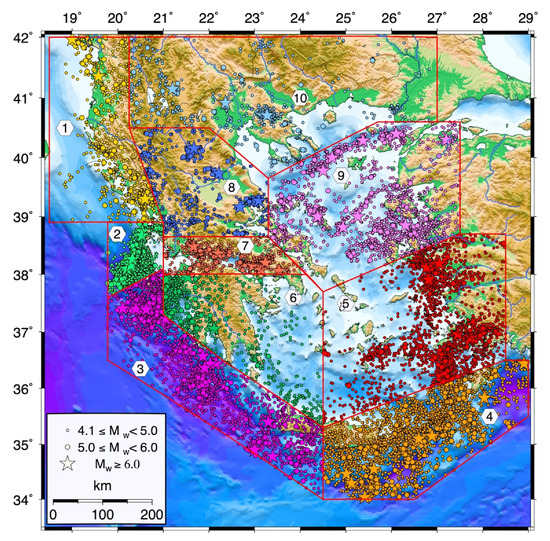
Figure 2.
Epicentral distribution of Greek seismicity with Mw 4.1 since 1975. Each different color illustrates the earthquakes of the 10 distinctive sub-areas that the broader Aegean region is divided (the borders of each sub-area are denoted with red polygons).
We divided the Hellenic Subduction Zone into two distinctive sub-areas, namely sub-areas 3 and 4, comprising the western and eastern parts of the Hellenic Subduction Zone, respectively. The Western Hellenic Arc is characterized by pure thrust fault plane solutions (Figure 1), in which the maximum compression, P-axis is oriented NNE–SSW along the Hellenic Arc, keeping the same orientation without being normal to the orientation of the subduction front. In the eastern part of the Hellenic Subduction Zone (sub-area 4) the available focal mechanisms evidence a more oblique motion.
The central part of the Aegean Sea, belonging to the extensional back arc area, is also separated into the eastern and western (including Peloponnese) parts, forming sub-areas 5 and 6, respectively. The Corinth Gulf, which is one of the most rapidly extending rifts worldwide, constitutes sub-area 7, while the central Greek mainland, is sub-area 8. Although all the four sub-areas belong to the extensional N–S back arc stress field, they are separated due to the fact that each of them constitutes distinctive and interconnected fault zones with different deformation rates [26].
The North Aegean Sea area is sub-area 9, comprising the right-lateral strike-slip North Aegean Trough Fault Zone (NATFZ), constituting the continuation of the North Anatolian Fault into the Aegean Sea [27], along with its major sub-parallel strands to the south, which are terminated to the west by the normal faults on the Greek mainland. It is characterized by dextral focal mechanisms with extensional components as well [28].
Northern Greece and the broader Balkans area constitute the 10th sub-area. It is a comparatively low seismicity area with the axis of maximum extension, T, to rotate from the N–S to an NE–SW orientation as one moves from its easternmost part to the west.
3. Data and Methodology
For the statistical correlations and the distribution fitting investigations on the 10 sub-region seismicity levels, we selected an earthquake catalog comprising the Mw 4.1 events that occurred in the territory of Greece during 1975–2021, which we have taken from the regional catalog compiled by the Geophysics Department of the Aristotle University of Thessaloniki (Available online: http://geophysics.geo.auth.gr/ss (accessed on 30 April 2022)). The earthquake magnitudes are expressed in moment magnitude scale (Mw), as obtained directly from waveform modeling or equivalent Mw based on scaling relations suggested by Papazachos et al. [29]. We divided the catalog into 10 sub-catalogs corresponding to the 10 distinctive sub-areas. Figure 2 shows the epicentral distribution of the earthquakes comprised in each sub-catalog with different colors for each sub-area for the reader’s ease. For each sub-catalog the samples of the earthquake interevent times, ΔT, data are then defined for earthquakes with magnitude thresholds of 0.1 bin increment, starting from Mw4.1 (ΔT1, ΔT2, … for the magnitude thresholds of Mw 4.1, Mw 4.2, … and so on for each sub-area). These data sets are the inputs for applying the methodology, which is described below.
We seek for the threshold magnitude, Mthr, of a certain data set, above which the interevent times are proved to be independent. For this purpose, we investigated the correlation of ΔT in each subset, with the subsets being created for certain magnitude bins. We examined the correlations by calculating the Autocorrelation (ACF) and Partial Autocorrelation (PACF) functions, a widely used approach for the same purpose (e.g., [30] for global earthquake data; [31] in induced seismicity of Poland).
The Autocorrelation Function (ACF),
where n is the number of the observations, k is the number of the lags and is the mean value of the observations, and is used for the investigation of correlations between past and future values of a given time series by assuming a confidence level (the 95% confidence level in the current application). If a certain ρκ value at lag k exceeds the 95% confidence interval then the given time series could be considered as correlated for the specific lag, otherwise, it could be considered statistically independent. Then, the possible correlations detected by the ACF can be confirmed in the same way based on the values of the Partial Autocorrelation Function that are given by
where for j = 1, 2, …, k.
Additionally, the Ljung–Box Q-test [32], which is a modified version of the Box–Pierce Portmanteau test, is applied as an alternative method to investigate correlations among ΔT. This test is implemented under the null hypothesis that the time series exhibits no autocorrelation for a fixed number of lags, L, against the alternative that some (statistically significant) autocorrelation exists. The test statistic is given by
The asymptotic distribution of Q is Chi-square (x2) with L degrees of freedom. If the statistic of the test for the given lag L is less than the critical value of the Chi-square (Qstat < Qcritical), the null hypothesis cannot be rejected.
For further confirmation of the possible crossover Mthr and for comparing our results with an independent method, we applied the Detrended Fluctuations Analysis [33] in all the 10 sub-regions. DFA is implemented under the hypothesis that if a given time series is correlated then the fluctuation function, F(n), follows an increasing power-law trend according to the factor nα (F(n)~nα), where n is the size of the window and α is the scaling exponent. If the value of the exponent α is larger than 0.5 (α > 0.5) then the data sample is positively correlated, whereas if α is smaller than 0.5 (α < 0.5) the data are negatively correlated (anti-correlated). For the case when the exponent α is equal to 0.5 (α = 0.5), the sample could be considered statistically independent. The exponent α is calculated as the slope of the linear regression of the logarithm of the fluctuation function, F(n), against the logarithm of the window size n.
The next step after the detection of the Mthr, above which the ΔT becomes statistically uncorrelated, is the determination of the best performed statistical distribution that each ΔT sample follows. Over the years, many statistical distributions such as the Weibull [34], the Lognormal [35,36], the Stretched Exponential [37] and the Gamma distribution [7,38] have been proposed. In this study, we applied the four most popular statistical distributions in the relevant studies (e.g., [39,40]), namely the Weibull, the Gamma, the Lognormal and the Exponential, to each ΔT data set for the 10 sub-areas. The probability density functions (pdf) of the four candidate distributions are given in Table 1. The parameter estimation for each distribution is achieved via the application of the Maximum Likelihood Estimation (MLE) method using the respective log-likelihood formulae [41].

Table 1.
Definitions of the probability density functions (pdf) of the Gamma, Lognormal, Weibull and Exponential distributions applied in the statistically independent interevent times data, ΔT, of the 10 sub-areas of broader Aegean region.
In order to compare the distribution’s performance and select the one that best fits the observations, we applied the Anderson–Darling non-parametric goodness of fit test (A–D test) [42]. The A–D test is implemented by calculating the distance, A2, between the empirical cumulative distribution function (ecdf) and the cumulative distribution function (cdf) of the distribution applied to the data. The A–D test statistic is given by
where {x1, x2, ..., xn} are the ordered sample data points, n is the number of observations and F is the cdf of the distribution under study. The test compares the quantity A2 with a critical value, c, under the null hypothesis that the data are distributed according to F. If A2 is less than or equal to the critical value, then the null hypothesis cannot be rejected. The decision of rejecting or not the null hypothesis in the present study is based on the obtained p-values, compared with the significance level, which is equal to 0.05 (α = 0.05). If the p-value is greater than α (p-value > α) then the null hypothesis can not be rejected. On the contrary, if the p-value is lower than α (p-value < α) the null hypothesis can be rejected.
To further compare the four distributions, we calculated the Akaike [43] and Bayesian [44] Information Criteria (AIC and BIC, respectively). From these calculations, the distribution that displays the best performance is the one with the minimum value of the criterion in both cases. The values of AIC and BIC are given by
and
where stands for the value of the log-likelihood function obtained from the MLE approach, k is the number of parameters of the distribution and n is the number of the observations.
4. Application
4.1. Identifying the Earthquake Interevent Time Correlations
The detection of the correlations is investigated through time series analysis. Specifically, the ACF and PACF values, along with the statistics of Ljung–Box Q-test are sequentially applied for each ΔTi data sample (ΔT1, ΔT2, …, ΔTn for Mw 4.1, Mw 4.2, …, respectively) for a given sub-area until the temporal crossover between correlated and statistically independent events is determined. It is worth mentioning that the 95% confidence intervals of ACF and PACF are calculated separately for each data sample ΔTi, which obtains a different length.
Figure 3, Figure 4 and Figure 5 illustrate the results of the correlation analysis for the ΔT data set for the central Ionian Islands area (sub-area 2). The values of ACF (Figure 3) exhibit strong positive autocorrelation until the magnitude threshold Mthr4.6 (Figure 3a–f). From this Mthr onwards, the autocorrelation becomes weaker (Figure 3g,h) until Mthr 4.9 (Figure 3i) when no significant autocorrelations of any lag are recorded, and the relevant samples of ΔT can be considered statistically uncorrelated. The values of PACF (Figure 4) confirm this crossover between correlated and statistically independent events at the magnitude threshold of Mthr 4.9.
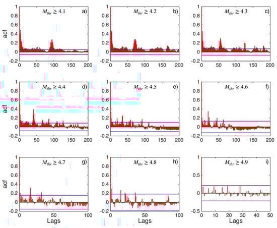
Figure 3.
ACF values (red stems) and their 95% confidence intervals (blue lines) for central Ionian Islands (sub-area 2) for magnitude thresholds (Mthr) varying from 4.1 to 4.9 (subplots a–i).
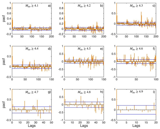
Figure 4.
PACF values (orange stems) and their 95% confidence intervals (blue lines) for central Ionian Islands (sub-area 2) for magnitude thresholds (Mthr) varying from 4.1 to 4.9 (subplots a–i).
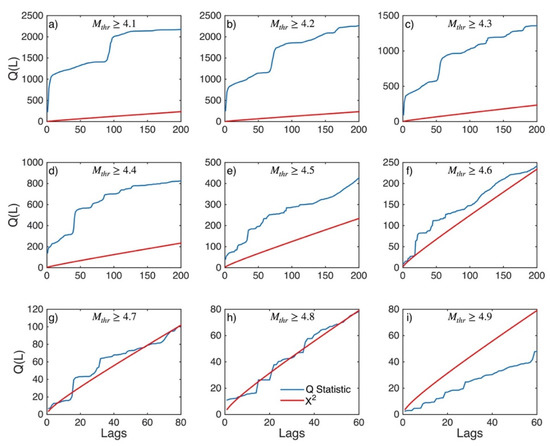
Figure 5.
Statistics of Ljung–Box Q-test (blue lines) and the critical values for the X2 distribution (red lines) for central Ionian Islands (sub-area 2) for magnitude thresholds (Mthr) varying from 4.1 to 4.9 (subplots a–i).
For securing that the finding of the memory weakening as the magnitude threshold increases is not biased because of the progressive decrease in the data samples length, the computation of the number of lags exceeding the respective level of significance over the total number of lags for both the ACF and PACF values is implemented. The ΔT data samples of this sub-region exhibit an increase in the ratio for the ACF values from 0.33 to 0.60 for the Mthr4.1 and Mthr4.2, respectively. From an Mthr4.3 and above we observe a systematic decrease in this ratio for ACF values. We obtained the same results for the ratio related to the respective values of PACF. Taking into account these results, it could be stated that the smaller length of the respective data samples as the Mthr values increase does not bias the results of the ACF and PACF calculations, implying weakening of the memory with respect to the increase in magnitude threshold.
The results of the Ljung–Box Q-test (Figure 5) unveil the same temporal behavior of the ΔT data samples. Specifically, it is observed that the statistic of the test (Qstat; blue lines in Figure 5) is much larger than the critical value (Qcritical; red lines in Figure 5) of the Chi-square distribution, and consequently, the null hypothesis that the ΔT data samples are independent can be rejected up to Mthr 4.8 (Figure 5a–h). The ΔT data samples in which the Q statistic is clearly smaller than the critical value is again one for the Mthr 4.9 earthquakes (Figure 5i), confirming the results of the ACF and PACF calculations. In this respect, the magnitude threshold above which the ΔT data of the central Ionian Islands appear statistically independent is for the Mthr 4.9 earthquakes.
Table 2 presents the results of the aforementioned workflow for the detection of the temporal crossover among correlated and statistically independent earthquakes for the 10 sub-areas. In all the 10 cases, the results of ACF–PACF analysis are in excellent agreement with those of the Ljung–Box Q-test (the detailed results of both ACF–PACF analysis and the Ljung–Box Q-test are given graphically in Appendix A). The temporal crossover of the earthquakes interevent times data ranges from Mthr 4.7 up to Mthr 5.1. The lower magnitude threshold (Mthr4.7) is observed in the southwest Aegean Sea and Peloponnese (sub-area 6), whereas the largest (Mthr 5.1) in western Greece and Albania (sub-area 1). Two out of the ten sub-areas (western Hellenic Arc and northern Greece and Balkans) are exhibiting temporal crossover for Mthr 4.8 threshold. Similarly, the ΔT data samples of sub-areas 2 and 7, namely the central Ionian Islands and Corinth Gulf, respectively, are statistically independent at Mthr 4.9 thresholds. The eastern Hellenic Arc, southeast Aegean Sea, central Greece and North Aegean Sea (sub-areas 4, 5, 8 and 9, respectively) are exhibiting a temporal crossover for earthquakes with Mthr 5.0.
Table 2.
Summary of the identification of the magnitude threshold (Mthr) above which interevent time data, ΔT, are statistically independent for the 10 sub-areas of the broader Aegean region.
To support these results, the Detrended Fluctuations Analysis (DFA) is performed for all sub-regions and Mthr values, in which the ACF–PACF analysis and Ljung–Box Q-test are applied. Figure 6 summarizes the results of the calculation of the exponent α for each sub-region versus the respective Mthr values. In all cases, a systematic decrease in the exponent α with an increase in the magnitude threshold can be observed. In all cases, α ranges from values that indicate strong positive correlations (around 0.8) to ones that reveal weaker correlations or statistically independent behavior (from 0.65 to 0.33). More specifically, exponent α is obtaining values near 0.5 for the highest Mthr values (except in the case of sub-region 9, which is equal to 0.67). These latter results are in very good agreement with the initially presented ones of the ACF–PACF analysis and Ljung–Box Q-test.
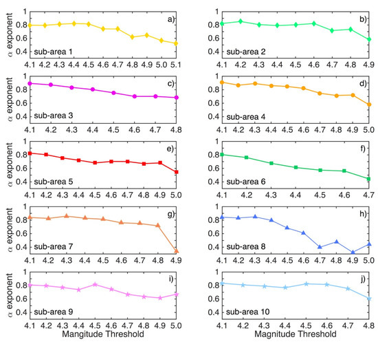
Figure 6.
Exponent α of Detrended Fluctuations Analysis as a function of Mthr for the 10 sub-areas (subplots a–j).
4.2. Distribution of the Statistically Independent Earthquake Interevent Times
After the detection of the magnitude thresholds above where the ΔT intervals are considered statistically independent, the statistical distribution of those data sets is investigated, with the application of the Weibull, Lognormal, Gamma and Exponential distributions. The parameters of each distribution are estimated via the MLE method according to their respective formulations, along with their 95% confidence intervals. Table 3 and Table 4 present the estimation results, along with the respective 95% confidence intervals and the values of the negative log-likelihood functions for sub-areas 1–5 and 6–10, respectively. An interesting point arising from the MLE approach is that the shape parameters of both the Gamma and Weibull distributions, k and b, respectively, obtain values below one in all cases (in all 10 sub-areas). This is an indicator of a clustering-type behavior of earthquake occurrence [45].
Table 3.
MLE parameters estimates, 95% confidence intervals, log-likelihood values calculation, Akaike and Bayesian Information Criteria calculated values (AIC and BIC, respectively), along with the estimated p-values of the Anderson–Darling Goodness of Fit test for the four applied statistical distributions on the statistically independent interevent times data, ΔT, of the sub-areas 1 to 5.
Table 4.
MLE parameters estimates, 95% confidence intervals, log-likelihood values calculation, Akaike and Bayesian Information Criteria calculated values (AIC and BIC, respectively), along with the estimated p-values of the Anderson–Darling Goodness of Fit test for the four applied statistical distributions on the statistically independent interevent times data, ΔT, of the sub-areas 6 to 10.
The Anderson–Darling (A–D) test is then applied to each sample in order to compare the distributions derived via the MLE parameter estimates and empirical cdf (Figure 7 and Figure 8 for sub-areas 1–5 and 6–10, respectively). Results of the A–D goodness of fit test (Table 3 and Table 4) show that in all cases the Exponential distribution can be rejected since the respective p-values are getting lower than the 0.05 level of significance (p-value < 0.05). Similarly, the Lognormal distribution is also rejected in 8 out of 10 cases. The rejected distributions report p-values larger than 0.05 for the central Ionian Islands and central Greece areas (sub-areas 2 and 8; Table 3). The Gamma and Weibull distributions perform better than the others in all the 10 ΔT data sets. Gamma distribution exhibits slightly better performance than the Weibull since the respective p-values are always larger than the ones of Weibull. These results are also confirmed by the obtained values of both Information Criteria (AIC and BIC; Table 3 and Table 4). In all 10 cases, the Gamma distribution is the one that reports the minimum values for both criteria.
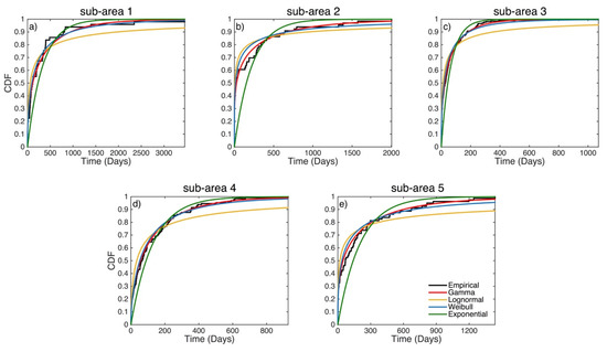
Figure 7.
Comparison of empirical cdf (black lines) and the cdfs of Gamma (red lines), Lognormal (yellow lines), Weibull (blue lines) and Exponential (green lines) applied distributions for sub-areas 1 to 5 (subplots a–e).
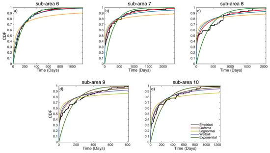
Figure 8.
Comparison of empirical cdf (black lines) and the cdfs of Gamma (red lines), Lognormal (yellow lines), Weibull (blue lines) and Exponential (green lines) applied distributions for sub-areas 6 to 10 (subplots a–e).
Summarizing the results of the comparison of the distributions, although both the Gamma and Weibull distributions can be accepted according to the A–D test in all cases (also the Lognormal one in the data sampled of sub-areas 2 and 8), the p-values of the test are smaller for the Gamma distribution. The values of AIC and BIC further confirm that Gamma distribution best fits the data since the relevant values are the lowest among the four. By combining the results of the A–D test with those of the information criteria, we found that the Gamma distribution fits better than the other three distributions for all data sets. This result is in agreement with Corral’s analysis [7,8], where the earthquake interevent times follow a universal scaling law independent of the region and the Mc, and can be modeled by the Gamma distribution.
As already stated, the estimated value of shape parameter, k, of Gamma distribution is found to be smaller than one in all the 10 ΔT data samples, independent of the temporal crossover magnitude threshold. Specifically, k ranges from 0.22 to 0.54 in the 10 sub-areas. This is an interesting finding from a seismological point of view because k plays an important role in earthquake occurrence applications; it could be considered the regulation parameter of the earthquake occurrence process [45]. Specifically, if k < 1, the temporal behavior of seismicity could be considered clustered, whereas if k > 1, the process tends to be quasi-periodic. In the case of k = 1, the process is neither periodic nor clustered, representing the memory-less Poisson process. In this respect, the estimated values of k indicate that although the ΔT data are statistically independent, there is still a weak inherent memory. This implies that earthquake interevent times above the given magnitude threshold of the temporal crossover are members of a renewal process, instead of the memory-less Poisson one.
5. Conclusions
The detection of the threshold magnitude, Mthr, above which the earthquake interevent times, ΔT, might be considered statistically independent, is investigated through the ACF and PACF values along with the application of the Ljung–Box Q-test in 10 distinctive sub-areas of the Greek territory. The analysis revealed that in all cases the results of the Ljung–Box Q-test adequately agree with the results derived by ACF and PACF. Detrended Fluctuations Analysis results further confirm the weakening of the memory as the Mthr of earthquake interevent time data increases. The obtained temporal crossover of the ΔT data ranges from Mthr 4.7 up to Mthr 5.1 in the 10 sub-areas. These findings are statistically very important because one can determine above which magnitude threshold the property of mutual independence is fulfilled. This independency property concerns either the events occurring in two different time intervals or only the occurrence time of the last event but not the full seismicity history. The proposed workflow for the investigation of the crossover behavior of ΔT data is easy to apply and capable of providing reliable results aimed at fixing the methodological issue of statistical independence. In other words, it could be considered as a routine initial step before a certain stochastic model application in earthquake interevent time data.
Once the magnitude thresholds above which the ΔT data samples are statistically independent are identified, the Gamma, Weibull, Lognormal and Exponential distributions are applied and compared in the respective data samples in order to model their temporal behavior. The comparison, which was implemented via the combination of the A–D goodness of fit test and the values of AIC and BIC criteria, revealed that the Gamma distribution exhibits the best performance. This latter result agrees with the analysis performed by Corral [7,8], who claimed that the earthquake interevent times follow a universal scaling law which could be represented by the Gamma distribution. This fact implies that the ΔT can be described better with a general renewal process rather than the Markovian Poisson process.
The values of the shape parameter, k, of Gamma distribution, which characterizes the seismic process, in all cases are estimated as k < 1 implying a clustering behavior of seismicity. In such cases, the earthquake occurrence probability soon after a strong earthquake is high, and most events occur at times less than the mean interevent time.
It is notable that sub-areas with low seismic activity are associated with larger values of k. In more detail, the largest estimated value of k is equal to 0.54 in the southwestern Aegean Sea and Peloponnese (sub-area 6), an area with considerably lower seismicity than the Corinth Gulf (sub-area 7) and North Aegean Sea (sub-area 9), in which the estimated k values are equal to 0.27 and 0.25, respectively. The smallest value of k (k = 0.22) is estimated in the central Ionian Islands (sub-area 2), which exhibits the highest moment rate in the Mediterranean region.
This study’s results provide information on the temporal behavior of the ΔT of moderate to large earthquakes over a sufficiently long period (1975–2021). These findings might be potentially used for both additional statistical applications (e.g., Stress Release applications), in which the need for documenting the independency magnitude cut-off is necessary, and as initial earthquake occurrence forecast models in intermediate time scales, which can be considered as inputs for improving regional seismic hazard assessment investigations (e.g., [46]).
Author Contributions
Conceptualization, C.K., G.T., E.P. and V.K.; data curation, C.K., E.P. and V.K.; formal analysis, C.K., G.T., E.P. and V.K.; investigation, C.K.; methodology, C.K. and G.T.; Validation, C.K.; writing—original draft, C.K.; writing—review and editing, C.K., G.T., E.P. and V.K. All authors have read and agreed to the published version of the manuscript.
Funding
This research received no external funding.
Institutional Review Board Statement
Not applicable.
Informed Consent Statement
Not applicable.
Data Availability Statement
The regional earthquake catalog of the Geophysics Department of the Aristotle University of Thessaloniki is accessible from http://geophysics.geo.auth.gr/ss (last accessed on 30 April 2022). Fault plane solution data used in Figure 1 came from https://www.globalcmt.org/ (last accessed on 30 April 2022).
Acknowledgments
We greatly appreciate the editorial assistance of A. Zavyalov as well as the constructive comments of three anonymous reviewers who contributed to the improvement of the manuscript. The GMT software [47] is used for creating the maps. Some figures and calculations are produced using the MATLAB software (Available online: http://www.mathworks.com/products/matlab (last accessed on 30 April 2022)). Geophysics Department Contribution 962.
Conflicts of Interest
The authors declare no conflict of interest.
Appendix A
In this section the detailed results of both ACF–PACF analysis and the Ljung–Box Q-test are presented graphically for the nine sub-areas, except the ones in the Central Ionian Islands (sub-area 2), which are shown in the main body of the study.
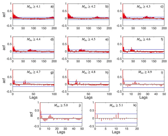
Figure A1.
ACF values (red stems) and their 95% confidence intervals (blue lines) for Western Greece and Albania (sub-area 1) for magnitude thresholds (Mthr) varying from 4.1 to 5 (subplots a–k).
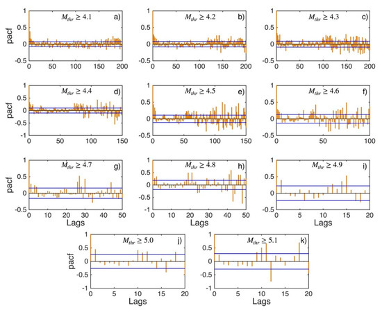
Figure A2.
PACF values (orange stems) and their 95% confidence intervals (blue lines) for Western Greece and Albania (sub-area 1) for magnitude thresholds (Mthr) varying from 4.1 to 5.1 (subplots a–k).
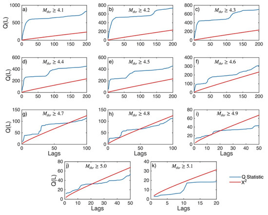
Figure A3.
Statistics of Ljung–Box Q-test (blue lines) and the critical values for the X2 distribution (red lines) for Western Greece and Albania (sub-area 1) for magnitude thresholds (Mthr) varying from 4.1 to 5.1 (subplots a–k).
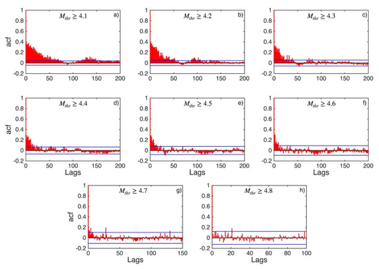
Figure A4.
ACF values (red stems) and their 95% confidence intervals (blue lines) for Western Hellenic Arc (sub-area 3) for magnitude thresholds (Mthr) varying from 4.1 to 4.8 (subplots a–h).
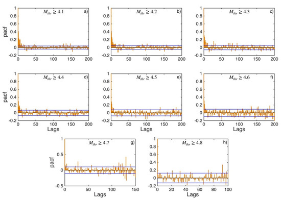
Figure A5.
PACF values (orange stems) and their 95% confidence intervals (blue lines) for Western Hellenic Arc (sub-area 3) for magnitude thresholds (Mthr) varying from 4.1 to 4.8 (subplots a–h).
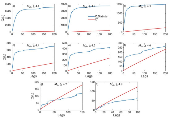
Figure A6.
Statistics of Ljung–Box Q-test (blue lines) and the critical values for the X2 distribution (red lines) for Western Hellenic Arc (sub-area 3) for magnitude thresholds (Mthr) varying from 4.1 to 4.8 (subplots a–h).
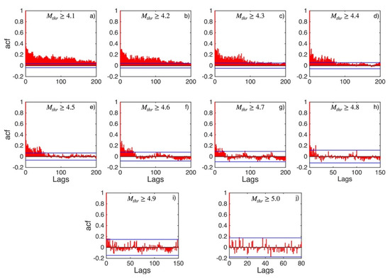
Figure A7.
ACF values (red stems) and their 95% confidence intervals (blue lines) for Eastern Hellenic Arc (sub-area 4) for magnitude thresholds (Mthr) varying from 4.1 to 5.0 (sublots a–j).
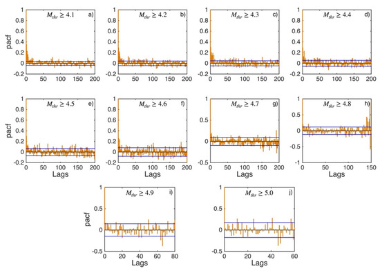
Figure A8.
PACF values (orange stems) and their 95% confidence intervals (blue lines) for Eastern Hellenic Arc (sub-area 4) for magnitude thresholds (Mthr) varying from 4.1 to 5.0 (subplots a–j).
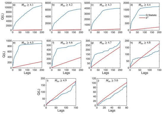
Figure A9.
Statistics of Ljung–Box Q-test (blue lines) and the critical values for the X2 distribution (red lines) for Eastern Hellenic Arc (sub-area 4) for magnitude thresholds (Mthr) varying from 4.1 to 5.0 (subplots a–j).
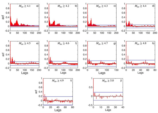
Figure A10.
ACF values (red stems) and their 95% confidence intervals (blue lines) for Southeast Aegean Sea (sub-area 5) for magnitude thresholds (Mthr) varying from 4.1 to 5.0 (subplots a–j).
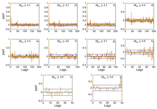
Figure A11.
PACF values (orange stems) and their 95% confidence intervals (blue lines) for Southeast Aegean Sea (sub-area 5) for magnitude thresholds (Mthr) varying from 4.1 to 5.0 (subplots a–j).
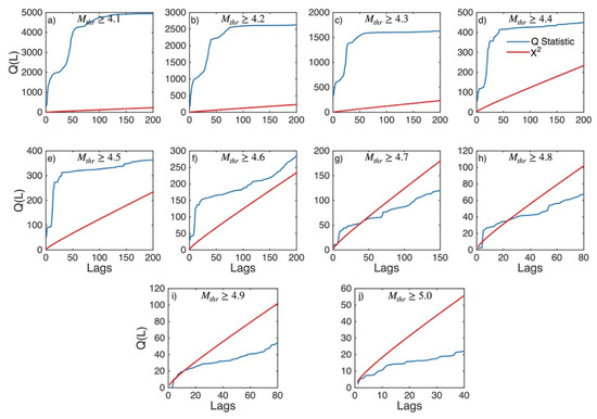
Figure A12.
Statistics of Ljung–Box Q-test (blue lines) and the critical values for the X2 distribution (red lines) for Southeast Aegean Sea (sub-area 5) for magnitude thresholds (Mthr) varying from 4.1 to 5.0 (subplots a–j).
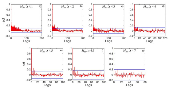
Figure A13.
ACF values (red stems) and their 95% confidence intervals (blue lines) for Southwest Aegean Sea and Peloponnese (sub-area 6) for magnitude thresholds (Mthr) varying from 4.1 to 4.7 (subplots a–g).
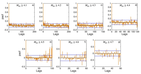
Figure A14.
PACF values (orange stems) and their 95% confidence intervals (blue lines) for Southwest Aegean Sea and Peloponnese (sub-area 6) for magnitude thresholds (Mthr) varying from 4.1 to 4.7 (subplots a–g).
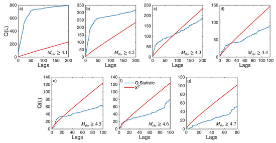
Figure A15.
Statistics of Ljung–Box Q-test (blue lines) and the critical values for the X2 distribution (red lines) for Southwest Aegean Sea and Peloponnese (sub-area 6) for magnitude thresholds (Mthr) varying from 4.1 to 4.7 (subplots a–g).
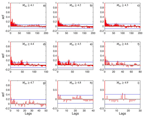
Figure A16.
ACF values (red stems) and their 95% confidence intervals (blue lines) for Corinth Gulf (sub-area 7) for magnitude thresholds (Mthr) varying from 4.1 to 4.9 (subplots a–i).
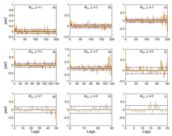
Figure A17.
PACF values (orange stems) and their 95% confidence intervals (blue lines) for Corinth Gulf (sub-area 7) for magnitude thresholds (Mthr) varying from 4.1 to 4.9 (subplots a–i).
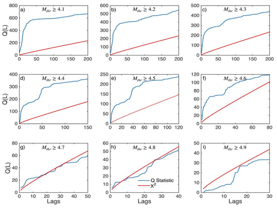
Figure A18.
Statistics of Ljung–Box Q-test (blue lines) and the critical values for the X2 distribution (red lines) for Corinth Gulf (sub-area 7) for magnitude thresholds (Mthr) varying from 4.1 to 4.9 (subplots a–i).
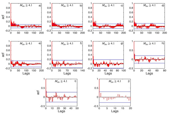
Figure A19.
ACF values (red stems) and their 95% confidence intervals (blue lines) for Central Greece (sub-area 8) for magnitude thresholds (Mthr) varying from 4.1 to 5.0 (subplots a–j).
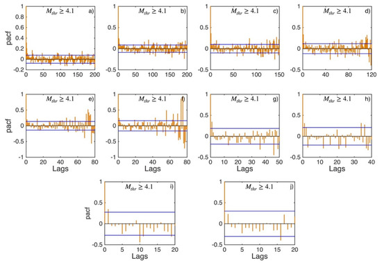
Figure A20.
PACF values (orange stems) and their 95% confidence intervals (blue lines) for Central Greece (sub-area 8) for magnitude thresholds (Mthr) varying from 4.1 to 5.0 (subplots a–j).
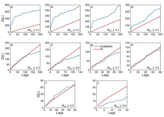
Figure A21.
Statistics of Ljung–Box Q-test (blue lines) and the critical values for the X2 distribution (red lines) for Central Greece (sub-area 8) for magnitude thresholds (Mthr) varying from 4.1 to 5.0 (subplots a–j).
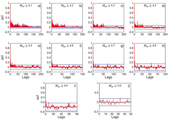
Figure A22.
ACF values (red stems) and their 95% confidence intervals (blue lines) for North Aegean Sea (sub-area 9) for magnitude thresholds (Mthr) varying from 4.1 to 5.0 (subplots a–j).
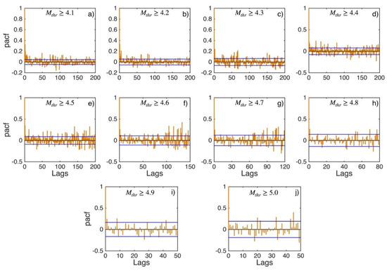
Figure A23.
PACF values (orange stems) and their 95% confidence intervals (blue lines) for North Aegean Sea (sub-area 9) for magnitude thresholds (Mthr) varying from 4.1 to 5.0 (subplots a–j).
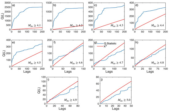
Figure A24.
Statistics of Ljung–Box Q-test (blue lines) and the critical values for the X2 distribution (red lines) for North Aegean Sea (sub-area 9) for magnitude thresholds (Mthr) varying from 4.1 to 5.0 (subplots a–j).
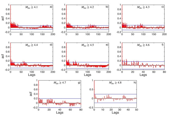
Figure A25.
ACF values (red stems) and their 95% confidence intervals (blue lines) for Northern Greece and Balkans (sub-area 10) for magnitude thresholds (Mthr) varying from 4.1 to 4.8 (subplots a–h).
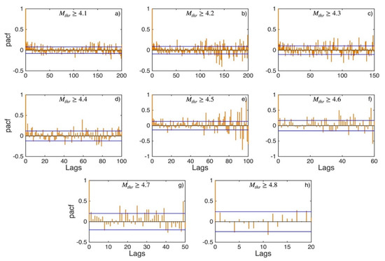
Figure A26.
PACF values (orange stems) and their 95% confidence intervals (blue lines) for Northern Greece and Balkans (sub-area 10) for magnitude thresholds (Mthr) varying from 4.1 to 4.8 (subplots a–h).
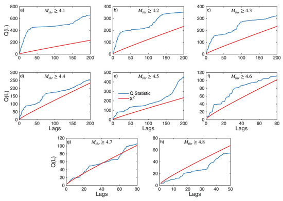
Figure A27.
Statistics of Ljung–Box Q-test (blue lines) and the critical values for the X2 distribution (red lines) for Northern Greece and Balkans (sub-area 10) for magnitude thresholds (Mthr) varying from 4.1 to 4.8 (subplots a–h).
References
- Kagan, Y.Y.; Jackson, D.D. Long-term probabilistic forecasting of earthquakes. J. Geophys. Res. 1994, 99, 13685–13700. [Google Scholar] [CrossRef]
- Dieterich, J. A constitutive law for rate of earthquake production and its application to earthquake clustering. J. Geophys. Res. 1994, 99, 2601–2618. [Google Scholar] [CrossRef]
- de Arcangelis, L.; Godano, C.; Grasso, J.R.; Lippiello, E. Statistical physics approach to earthquake occurrence and forecasting. Phys. Rep. 2016, 628, 1–91. [Google Scholar] [CrossRef]
- Gutenberg, B.; Richter, C. Frequency of earthquakes in California. Bull. Seismol. Soc. Am. 1944, 34, 185–188. [Google Scholar] [CrossRef]
- Omori, F. On the aftershocks of earthquakes. J. Coll. Sci. Imp. Univ. Tokyo 1894, 7, 111–200. [Google Scholar]
- Bak, P.; Christensen, K.; Danon, L.; Scanlon, T. Unified scaling law for earthquakes. Phys. Rev. Lett. 2002, 88, 178501. [Google Scholar] [CrossRef] [Green Version]
- Corral, A. Local distributions and rate fluctuations in a unified scaling law for earthquakes. Phys. Rev. E 2003, 68, 035102-1–035102-4. [Google Scholar] [CrossRef] [Green Version]
- Corral, A. Long-term clustering, scaling, and universality in the temporal occurrence of earthquakes. Phys. Rev. Lett. 2004, 92, 108501. [Google Scholar] [CrossRef] [Green Version]
- Molchan, G. Interevent time distribution in seismicity: A theoretical approach. Pure Appl. Geophys. 2005, 162, 1135–1150. [Google Scholar] [CrossRef] [Green Version]
- Saichev, A.; Sornette, D. Universal distribution of interearthquake times explained. Phys. Rev. Lett. 2006, 97, 078501. [Google Scholar] [CrossRef] [Green Version]
- Touati, S.; Naylor, M.; Main, I.G. Origin and nonuniversality of the earthquake interevent time distribution. Phys. Rev. Lett. 2009, 102, 168501. [Google Scholar] [CrossRef] [PubMed] [Green Version]
- Godano, C. A new expression for the earthquake interevent time distribution. Geophys. J. Int. 2015, 202, 219–223. [Google Scholar] [CrossRef]
- Ogata, Y. Statistical models for earthquake occurrence and residual analysis for point process. J. Am. Stat. Assoc. 1988, 83, 9–27. [Google Scholar] [CrossRef]
- Livina, V.N.; Havlin, S.; Bunde, A. Memory in the occurrence of earthquakes. Phys. Res. Lett. 2005, 95, 208501. [Google Scholar] [CrossRef] [Green Version]
- Lennartz, S.; Livina, V.N.; Bunde, A.; Havlin, S. Long-term memory in earthquakes and the distribution of interoccurrence time. EPL 2008, 81, 69001. [Google Scholar] [CrossRef] [Green Version]
- Fan, J.; Zhou, D.; Shekhtman, L.M.; Shapira, A.; Hofstetter, R.; Marzocchi, W.; Ashkenazy, Y.; Havlin, S. Possible origin of memory in earthquakes: Real catalogs and an epidemic-type aftershock sequence model. Phys. Rev. E 2019, 99, 042210. [Google Scholar] [CrossRef] [Green Version]
- Zhang, Y.; Fan, J.; Marzocchi, W.; Shapira, A.; Hofstetter, R.; Havlin, S.; Ashkenazy, Y. Scaling laws in earthquake memory for interevent times and distances. Phys. Rev. Res. 2020, 2, 013264. [Google Scholar] [CrossRef] [Green Version]
- Gkarlaouni, C.; Lasocki, S.; Papadimitriou, E.; Tsaklidis, G. Hurst analysis of seismicity in Corinth rift and Mygdonia graben (Greece). Chaos Solit. Fractals 2017, 96, 30–42. [Google Scholar] [CrossRef]
- Parsons, T.; Geist, E.L. Were global M≥8.3 earthquake time intervals random between 1900 and 2011? Bull. Seismol. Soc. Am. 2012, 102, 1583–1592. [Google Scholar] [CrossRef]
- Zhuang, J.; Harte, D.; Werner, M.J.; Hainzl, S.; Zhou, S. Basic models of seismicity: Temporal models. Community Online Resour. Stat. Seism. Anal. 2012, 1, 42. [Google Scholar] [CrossRef]
- Rahimi, M.; Zamali, A.; Ghotbi, A.R. The study of seismicity of Alborz (Northern Iran) and Zagros (Southern Iran) regions by using time series analysis. Acta Geophys. 2022, 70, 27–37. [Google Scholar] [CrossRef]
- Papazachos, B.C.; Comninakis, P.E. Geophysical and tectonic features of the Aegean arc. J. Geophys. Res. 1971, 76, 8517–8533. [Google Scholar] [CrossRef]
- LePichon, X.; Angelier, J. The Hellenic Arc and Trench system: A key to the neotectonic evolution of the eastern Mediterranean area. Tectonophysics 1979, 60, 1–42. [Google Scholar]
- Papazachos, B.C.; Papadimitriou, E.E.; Kiratzi, A.A.; Papazachos, C.B.; Louvari, E.K. Fault plane solutions in the Aegean Sea and the surrounding area and their tectonic implications. Boll. Geofis. Teor. Appl. 1998, 39, 199–218. [Google Scholar]
- Scordilis, M.; Karakaisis, G.; Karakostas, V.; Panagiotopoulos, D.G.; Comninakis, P.E.; Papazachos, B.C. Evidence for transform faulting in the Ionian sea: The Cephalonia island earthquake sequence of 1983. Pure Appl. Geophys. 1985, 123, 388–397. [Google Scholar] [CrossRef]
- Goldsworthy, M.; Jackson, J.; Haines, J. The continuity of active faults systems in Greece. Geophys. J. Int. 2002, 148, 596–618. [Google Scholar] [CrossRef] [Green Version]
- Armijo, R.; Meyer, B.; Hubert, A.; Barka, A. Westward propaga- tion of the North Anatolian fault into the northern Aegean: Timing and kinematics. Geology 1999, 27, 267–270. [Google Scholar] [CrossRef]
- Taymaz, T.; Jackson, J.; McKenzie, D. Active tectonics of the North and central Aegean Sea. Geophys. J. Int. 1991, 106, 433–490. [Google Scholar] [CrossRef]
- Papazachos, B.C.; Kiratzi, A.A.; Karakostas, B.G. Towards a homogeneous moment magnitude determination for earthquakes in Greece and the surrounding area. Bull. Seismol. Soc. Am. 1997, 87, 474–483. [Google Scholar] [CrossRef]
- Naylor, M.; Main, I.G.; Touati, S. Quantifying uncertainty in mean earthquake interevent times for a finite sample. J. Geophys. Res. 2009, 114, B01316. [Google Scholar] [CrossRef] [Green Version]
- Weglarczyk, S.; Lasocki, S. Studies of short and long memory in mining-induced seismic processes. Acta Geophys. 2009, 57, 696–715. [Google Scholar] [CrossRef]
- Ljung, G.; Box, G.E.P. On a Measure of Lack of Fit in Time Series Models. Biometrika 1978, 66, 67–72. [Google Scholar] [CrossRef]
- Peng, C.K.; Buldyrev, S.V.; Havlin, S.; Simons, M.; Stanley, H.E.; Goldberger, A.L. Mosaic organization of DNA nucleotides. Phys. Rev. E Stat. Phys. Plasmas Fluids Relat. Interdiscip. Topics 1994, 49, 1685. [Google Scholar] [CrossRef] [Green Version]
- Abaimov, S.G.; Turcotte, D.L.; Shcherbakov, R.; Rundle, J.B.; Yakovlev, G.; Goltz, C.; Newman, W.I. Earthquakes: Recurrence and interoccurrence Times. Pure Appl. Geophys. 2008, 165, 777–795. [Google Scholar] [CrossRef]
- Nishenko, S.P.; Buland, R. A generic recurrence interval distribution for earthquake forecasting. Bull. Seismol. Soc. Am. 1987, 77, 1382–1399. [Google Scholar]
- Werner, M.J.; Ide, K.; Sornette, D. Earthquake forecasting based on data assimilation: Sequential Monte Carlo methods for renewal point processes. Nonlinear Process. Geophys. 2011, 18, 49–70. [Google Scholar] [CrossRef]
- Altmann, E.G.; Kantz, H. Recurrence time analysis, long-term correlations, and extreme events. Phys. Rev. E 2005, 71, 1–9. [Google Scholar] [CrossRef] [Green Version]
- Udias, A.; Rice, J. Statistical analysis of microearthquake activity near San Andreas Geophysical Observatory, Hollister, California. Bull. Seismol. Soc. Am. 1975, 65, 809–827. [Google Scholar] [CrossRef]
- Mesimeri, M.; Kourouklas, C.; Papadimitriou, E.; Karakostas, V.; Kementzetzidou, D. Analysis of microseismicity associated with the 2017 seismic swarm near the Aegean coast of NW Turkey. Acta Geophys. 2018, 66, 479–495. [Google Scholar] [CrossRef]
- Coban, K.H.; Sayil, N. Conditional Probabilities of Hellenic Arc Earthquakes Based on Different Distribution Models. Pure Appl. Geophys. 2020, 177, 5133–5145. [Google Scholar] [CrossRef]
- Johnson, N.L.; Kotz, S.; Balakrishnan, N. Continuous Univariate Distributions, 2nd ed.; Wiley: New York, NY, USA, 1994; Volume 1, pp. 1–784. [Google Scholar]
- Anderson, T.W.; Darling, D.A. Asymptotic theory of certain ‘goodness-of-fit’ criteria based on stochastic processes. Ann. Math. Stat. 1952, 23, 193–212. [Google Scholar] [CrossRef]
- Akaike, H. A new look at the statistical model identification. IEEE Trans. Autom. Contr. 1974, 19, 716–723. [Google Scholar] [CrossRef]
- Schwarz, G. Estimating the dimension of a model. Ann. Stat. 1978, 6, 461–464. [Google Scholar] [CrossRef]
- Convertito, V.; Faenza, L. Earthquake Recurrence. In Encyclopedia of Earthquake Engineering; Beer, M., Kougioumtzoglou, I.A., Patelli, E., Siu-Kui Au, I., Eds.; Springer: Berlin, Germany, 2014; pp. 1–22. [Google Scholar]
- Mobarki, M.; Talbi, A. Spatio-temporal analysis of main seismic hazard parameters in the Ibero-Maghreb region using an Mw-homogenized catalog. Acta Geophys. 2022, 70, 979–1001. [Google Scholar] [CrossRef]
- Wessel, P.; Smith, W.H.F.; Scharroo, R.; Luis, J.; Wobbe, F. Generic mapping tools: Improved version released. EOS Trans. Am. Geophys. Union 2013, 94, 409–410. [Google Scholar] [CrossRef] [Green Version]
Publisher’s Note: MDPI stays neutral with regard to jurisdictional claims in published maps and institutional affiliations. |
© 2022 by the authors. Licensee MDPI, Basel, Switzerland. This article is an open access article distributed under the terms and conditions of the Creative Commons Attribution (CC BY) license (https://creativecommons.org/licenses/by/4.0/).