MLoF: Machine Learning Accelerators for the Low-Cost FPGA Platforms

Abstract

In Internet of Things (IoT) scenarios, it is challenging to deploy Machine Learning (ML) algorithms on low-cost Field Programmable Gate Arrays (FPGAs) in a real-time, cost-efficient, and high-performance way. This paper introduces Machine Learning on FPGA (MLoF), a series of ML IP cores implemented on the low-cost FPGA platforms, aiming at helping more IoT developers to achieve comprehensive performance in various tasks. With Verilog, we deploy and accelerate Artificial Neural Networks (ANNs), Decision Trees (DTs), K-Nearest Neighbors (k-NNs), and Support Vector Machines (SVMs) on 10 different FPGA development boards from seven producers. Additionally, we analyze and evaluate our design with six datasets, and compare the best-performing FPGAs with traditional SoC-based systems including NVIDIA Jetson Nano, Raspberry Pi 3B+, and STM32L476 Nucle. The results show that Lattice’s ICE40UP5 achieves the best overall performance with low power consumption, on which MLoF averagely reduces power by 891% and increases performance by 9 times. Moreover, its cost, power, Latency Production (CPLP) outperforms SoC-based systems by 25 times, which demonstrates the significance of MLoF in endpoint deployment of ML algorithms. Furthermore, we make all of the code open-source in order to promote future research.

1. Introduction

Machine Learning (ML) algorithms are effective and efficient in processing Internet of Things (IoT) endpoint data with well robustness [1]. As data volumes grow, IoT endpoint ML implementations have become increasingly important. Compared to the traditional cloud-based approaches, they can compute in real-time and reduce the communication overhead [2]. There are some researches deploying ML algorithms on System on Chip (SoC) based endpoint devices in industry and academia. For example, the TensorFlow Lite [3], X-CUBE-AI [4], and the Cortex Microcontroller Software Standard Neural Network (CMSIS-NN) [5] are three frameworks proposed by Google, STM, and ARM for pre-trained models in embedded systems. However, these solutions cannot achieve a balance among power consumption, cost-efficiency, and high-performance simultaneously for IoT endpoint ML implementations.

Field Programmable Gate Array (FPGA) devices have an inherently parallel architecture that makes them suitable for ML applications [6]. Moreover, some FPGAs have substantially close costs and leakage power compared to those of Microcontroller Unit (MCU). Therefore, FPGA can be an ideal target platform for IoT endpoint ML implementations. Nowadays, some researches and supports have been done for the deployment of ML algorithms on FPGAs. For instance, the ongoing AITIA, led by the Technical University of Dresden, KUL, IMEC, VUB, etc. [7], is a preliminary project that investigated the feasibility of ML implementations on FPGAs. On the other hand, in the industry, Xilinx and Intel have supported portions of the machine learning based Intellectual Property (IP) cores [8,9,10,11]. Unfortunately, these solutions are based on high-end FPGAs and require highly professional standards. It is difficult for many small and medium-sized corporations and individual developers to deploy their hardware platforms. Therefore, an ML library that can run on any FPGA platform is needed [12], especially those low-cost FPGAs. Low-cost FPGAs do not mean they have the lowest absolute value among all FPGAs, instead, they refer to the lowest-priced FPGA series in the most representative manufacturers. Meanwhile, the lack of comprehensive comparisons makes it difficult to demonstrate the benefits of FPGA ML implementations over conventional SoC-based solutions.

Therefore, we introduce Machine Learning on FPGA (MLoF) with a series of IP cores dedicated to low-cost FPGAs. The MLoF IP-cores are developed in Verilog Hardware Description Language (HDL) and can be used to implement popular machine learning algorithms on FPGAs, including Support Vector Machines (SVMs), K-Nearest Neighbors (k-NNs), Decision Trees (DTs), and Artificial Neural Networks (ANNs). The performance of seven FPGA producers (Anlogic *2, Gowin *1, Intel *2, Lattice *2, Microsemi *1, Pango *1, and Xilinx *1) is thoroughly evaluated using low-cost platforms. As far as we know, MLoF is the first case to implement machine learning algorithms on nearly every low-cost FPGA platform. Compared with the typical way of implementing machine learning algorithms on embedded systems, including NVIDIA Jetson Nano, Raspberry Pi 3B+, and STM32L476 Nucle, the advantage of MLoF is that it balances the cost, performance, and power consumption. Moreover, these IP cores are open-source, assisting developers and researchers in more efficient implementation of machine learning algorithms on their endpoint devices.

The contributions of this paper are as follows:

(1)

To the best knowledge of the authors, this is the first time that four ML hardware accelerator IP-cores are generated using Verilog HDL, including SVM, k-NN, DTs and ANNs. The source code of all IP-cores is fully disclosed at github.com/verimake-team/MLonFPGA;

(2)

The proposed IP-cores are deployed and validated on 10 mainstream low-cost and low-power FPGAs from seven producers to show its broad compatibility;

(3)

Our designs are comprehensively evaluated on FPGA boards and embedded system platforms. The results prove that low-cost FPGAs are ideal platforms for IoT endpoint ML implementations;

The rest of this paper is organized as follows: Section 2 reviews prior work on the hardware implementations of machine learning algorithms. Section 3 introduces details of the proposed MLoF IP series. Section 4 provides a comparison of various FPGA development platforms. Section 5 contains experiments and analyses. Section 6 concludes the research results and future works.

2. Related Work

For decades, the implementations of machine learning algorithms on low-cost embedded systems have been vigorously investigated. Due to the limited computing resources on embedded systems, these approaches tend to lack outstanding performance. However, FPGA is an effective solution for machine learning algorithms [13]. Saqib et al. [14] proposed a decision tree hardware architecture based on FPGA. It improves data throughput and resource utilization efficiency by utilizing parallel binary decision trees and a pipeline. A 3.5× computing speed is achieved while only 2952 Look-up Tables (LUTs) of resources are consumed via an 8-parallelism 4-stage pipeline. Nasrin Attaran et al. [15] proposed a binary classification architecture based on SVM and k-NN. Over 10× computing speed and 200× power-delay are obtained as compared with ARM A53. Gracieth et al. [16] proposed a 4-stage, low-power SVM pipeline architecture capable of achieving 98% of accuracy on over 30 classification tasks. It consumes only 1315 LUTs of resources and operates at a system frequency of 50 MHz. The aforementioned works introduce the deployment of ML algorithms on FPGA platforms, but there are still deficiencies: 1. None of the works integrate the mainstream ML algorithms for FPGA deployment; 2. None of the works compare the final results horizontally with other embedded platforms of various IoT terminals.

Due to the high inherent parallelism in FPGAs, more advanced machine learning algorithms, such as neural networks, are widely studied. Roukhami M et al. [17] proposed a Deep Neural Network (DNN) based architecture for classification tasks on low-power FPGA platforms. They thoroughly compared the performance with STM32 ARM MCU and designed a general communication interface for accelerators, such as SPI and UART. The entire acceleration process consumes only 25.459 mW of power with a latency of 1.99 s. Chao Wang et al. [18] proposed a Deep Learning Accelerating Unit (DLAU) that accelerates neural networks, e.g., DNN and CNN. Additionally, they developed an AXI-Lite interface for the acceleration unit to enhance its versatility. In general, the DLAU outperforms Cortex-A7 by 67%. Fen Ge et al. [19] developed a resource-constrained CNN accelerator for IoT endpoint SoCs that does not require any DSP resources. With a total resource overhead of 4901 LUTs, the data throughput reaches 6.54 GOP (Giga Operation per second). The above works present neural network-based FPGA deployments, but none of them is designed for low-cost FPGAs, which are oftentimes the most prevalent platforms used for IoT endpoints.

Although the previous works succeed in increasing the capability of endpoint computing by implementing only one or two machine learning algorithms on FPGAs, further analyses and comprehensive comparisons across low-cost FPGA platforms, as well as the integration of more commonly used machine learning algorithms are still required.

3. Machine Learning Algorithms Implementation on Low-Cost FPGAs

Normally, the post-process of IoT data mainly focuses on two tasks: Classifications and regressions [20]. By exploiting the parallelism and low power consumption of FPGAs, MLoF offers a superior solution for these workloads. Drawn from past designs, MLoF is designed with lower computation resources, and it includes a variety of common machine learning algorithms, namely ANN, DT, k-NN, and SVM. Details will be further presented in this section.

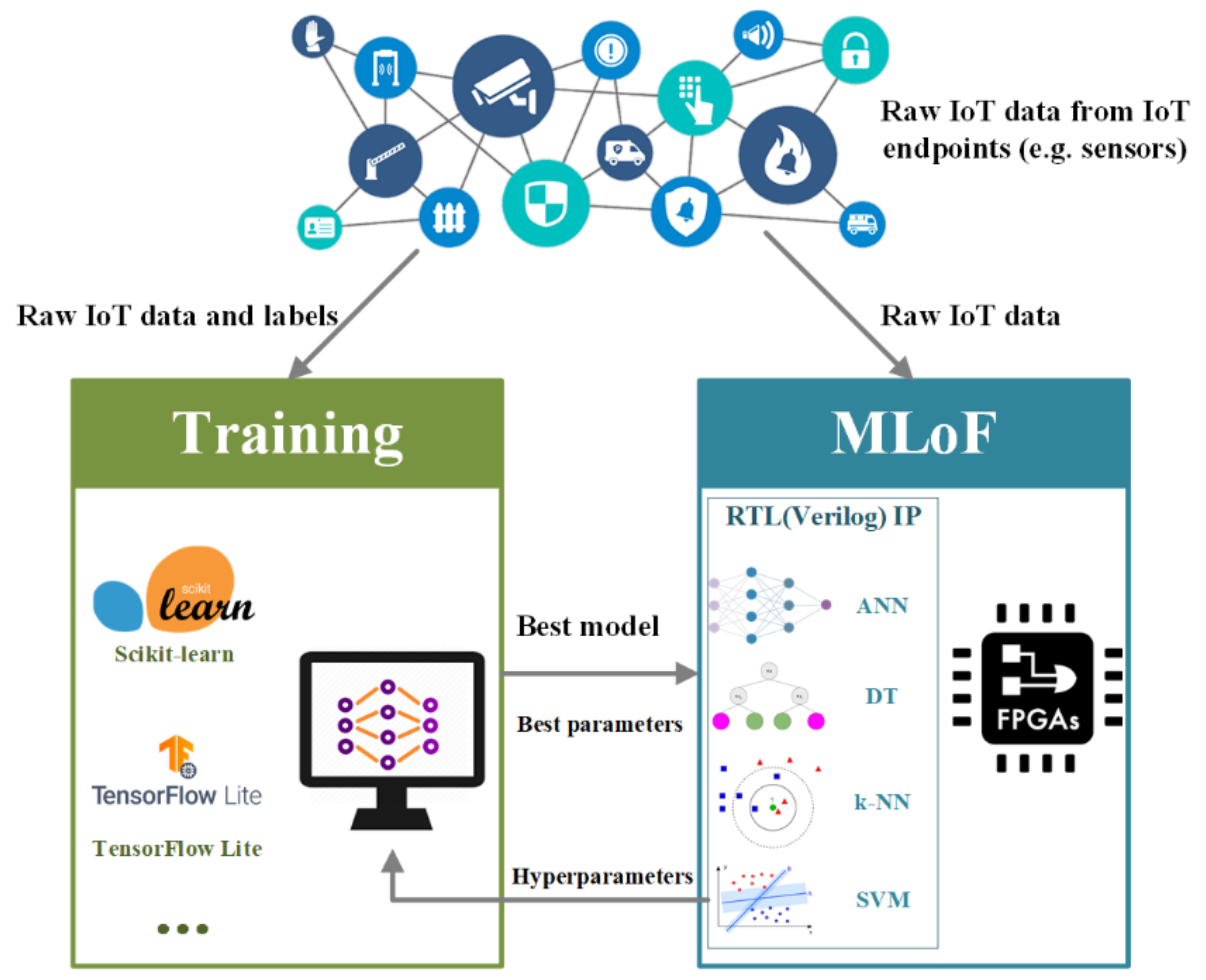
As shown in Figure 1, the system has consisted of the training and the MLoF modules as most machine learning models are used for inferencing and evaluating within IoT devices without requiring extensive training [21], all of the model training process is completed through PC. First, the IoT dataset is gained from the endpoints and will be sent to the training module. Then, an ML library (e.g., Scikit-Learn and TensorFlow Lite) [22] and an ML algorithm should be chosen as the first level of parameters. Thereafter, a set range of hyperparameters (the same set as in the MLoF module) are used to constrain the PC training process, as FPGA has limited local resources. Since hyperparameters are key features in ML algorithms [23,24,25], users could set them to different values to find the best sets for training according to Table 1. Next, with all the labeled data and hyperparameters, the best model and the best parameters (including the updated hyperparameters) are generated and sent to the MLoF module. After receiving and storing the parameters into ROM or external Flash, the algorithm is deployed on an FPGA. The language of FPGA is mainly Verilog HDL, thus the algorithms can literally be deployed on any known FPGA platform.

Figure 1. Block diagram of the MLoF system architecture.

Table 1. Configurable parameters.

ANN	DT	k-NN	SVM
Data width (max = 13);
Number of inputs (max = 16);	Data width (max = 13);	Data width (max = 13);	Data width (max = 13);
Number of hidden layers (max = 4);	Number of depth (max = 6);	Number of inputs (max = 16);	Number of inputs (max = 16);
Number of neurons in each hidden layer (max = 8);	Number of leaf nodes (max = 64);	Number of neighbors (max = 16);	Number of targets (max = 16)
Number of targets (max = 16);	Number of targets (max = 16)	Number of targets (max = 16)
Activation functions

In this paper, we selected six datasets, the four most representative ML algorithms, and deployed them on 10 low-cost FPGAs, with a total of 240 combinations. The experiments and evaluations are described in detail in Section 5.

3.1. Artificial Neural Networks (ANN)

3.1.1. Overall Structure of ANN

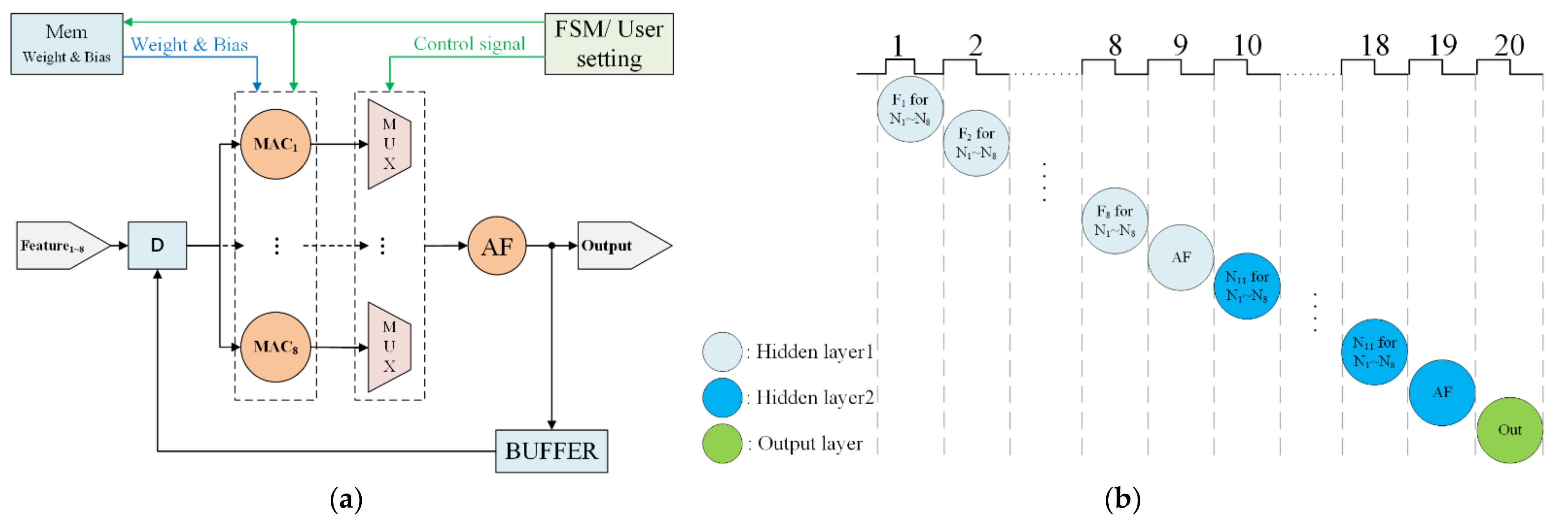
The implementation of ANN, for example, with eight inputs and two hidden layers (eight neurons within each layer) is shown in Figure 2a. This ANN model includes a Memory Unit (Mem), a Finite State Machine (FSM), eight Multiplying Accumulator (MAC) computing units, Multiplexers (MUX), an Activation Function Unit (AF), and a Buffer Unit (BUFFER). The Memory Unit (Mem) stores the weights and biases after training. The FSM manages the computation order and the data stream. The MAC units are designed with multipliers, adders, and buffers for multiplying and adding operations within each neuron. Here, we implement eight MAC blocks to process in parallel the multiplication of the eight neurons. Initially, features are serially entered for registration. Then, the MAC is used to sequentially process the ANN from the first input feature to the eighth feature on the first hidden layer (Figure 2b). Next, the second hidden layer is sequentially processed from the first hidden neuron to the eighth neuron. Finally, we process the output by the activation function. As demonstrated in Figure 3, the multiplexers (MUX) allocate the data stream. The AF computes the activation functions, which will be discussed in Section 3.1.2. The buffer stores data computed from each neuron.

Figure 2. ANN algorithm implementation. (a) Block diagram of ANN. (b) Scheduling of the ANN processing.

Figure 3. Block diagram of MAC.

The entire procedure for performing a hardware-based ANN architecture is described below. First, eight features are serially inputted to an ANN model. Each feature is entered into eight MAC units simultaneously and multiplications for eight neurons in the first layer are then completed. An inner buffer is used to store the multiplication results. Next, all eight results are added to a user-specified activation function. The output is further stored in the buffer unit as the input of the next hidden layer. Finally, the results are exported from the output layer following the second hidden layer.

3.1.2. Activation Function

The activation function is required within each neuron, which introduces non-linearity into the ANN, resulting in better abstract capability. Three typical activation functions include the Rectified Linear Unit (ReLU), the Hyperbolic Tangent Function (Tanh), and the Sigmoid Function [26]. All of three activation functions listed above are developed in hardware, and details are described as follows.

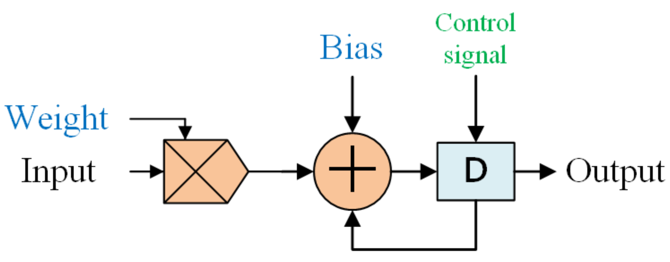
Rectified Linear Unit (ReLU)

The mathematical representation of the ReLU is described as Equation (1):

$$\mathrm{ReLU}\left(x\right)=\left\{\begin{array}{c}x, x>0\\ 0,x\le 0\end{array}\right.$$

(1)

The hardware implementation is shown in Figure 4 with a comparator and a multiplexer [27]:

Figure 4. Block diagram of ReLU.

Hyperbolic Tangent Function (Tanh)

The mathematical representation of the Tanh function is described as Equation (2):

$$\text{Tanh}\left(x\right)=\frac{e^x-e^{-x}}{e^x+e^{-x}}$$

(2)

This cannot be achieved directly in the hardware using HDL. Therefore, we fit this functionality separately with five sub-intervals [28]. We divide the interval of [0, +∞] into five sub-intervals: [0, 1], (1, 2], (2, 3], (3, 4], (4, +∞). Table 2 contains the heuristic functions used to fit the Tanh function for each sub-interval. The performance of each sub-interval is shown in Figure 5 with an error kept within an acceptable range. The sub-intervals enable the Tanh function to be implemented using only adders and multipliers.

Table 2. Fitting function at different intervals.

Numerical Interval	Function	Absolute Error
[0, 1]	$y=-0.3275x^2+1.0977x-0.0038$	0.0038
(1, 2]	$y=-0.1690x^2+0.7021x+0.2324$	0.0039
(2, 3]	$y=-0.0282x^2+0.1703x+0.7370$	0.0055
(3, 4]	$y=-0.0039x^2+0.0313x+0.9363$	0.0101
$(4, +\infty$)	1	/

Figure 5. The images of the fitting effect of these functions. (a) Numerical interval [0, 1]. (b) Numerical interval (1, 2]. (c) Numerical interval (2, 3]. (d) Numerical interval (3, 4].

Sigmoid Function

The mathematical representation of the Sigmoid function is described as Equation (3):

$$\mathrm{Sigmoid}\left(x\right)=\frac{1}{1+e^{-x}}$$

(3)

Similar to the Tanh function, the Sigmoid function cannot be implemented directly in the hardware using HDL, as well. The Sigmoid function is equivalent to the tanh function [29] when the transformation in Equation (4) is applied:

$$\mathrm{Sigmoid}\left(x\right)=\frac{\text{Tanh}\left(\raisebox{1ex}{$x$}\!\left/ \!\raisebox{-1ex}{$2$}\right.\right)+1}{2}$$

(4)

This transformation can be implemented easily on the hardware using a shift operation and an adder based on the tanh function.

3.2. Decision Tree (DT)

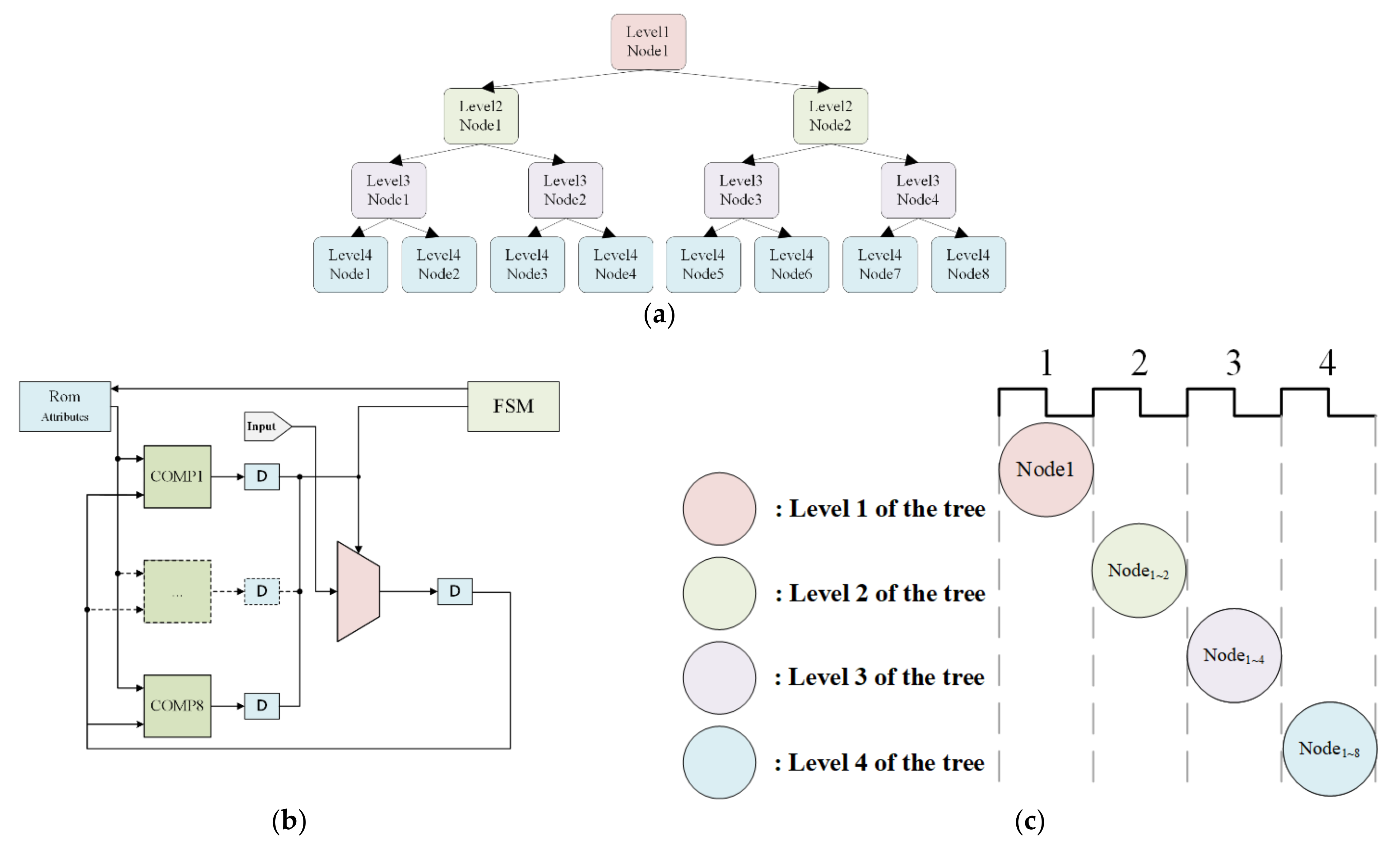
Figure 6 illustrates the implementation of DT with multiple inputs, a depth of four, and a maximum of eight nodes on each layer. The DT consists of a Memory Unit (Rom), a Finite State Machine (FSM), eight compare units, and a dispatcher. The memory unit is used to store nodes’ parameters from PC training. The FSM is used to determine which input node to use next based on the output. The compare unit serves as the selecting node. The distributor is used to distribute the input to each node.

Figure 6. DT algorithm implementation. (a) The sample decision tree. (b) Block diagram of DT. (c) Scheduling of the DT processing.

3.3. The k-Nearest Neighbors (k-NN)

3.3.1. Overall Structure of k-NN

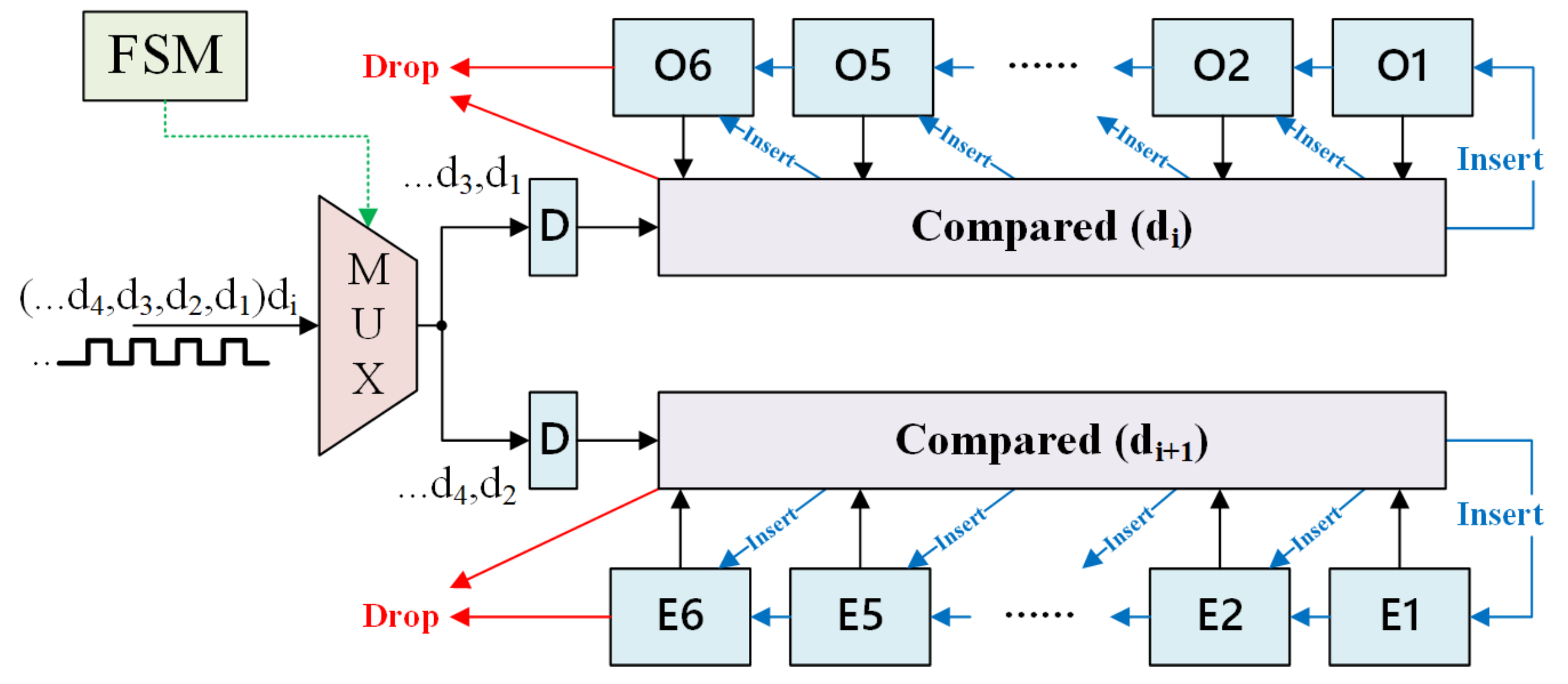
The k-NN method is used to classify the samples based on their distances. In this case, we use the squared Euclidean distance as defined in Equation (5). The structure of k-NN is demonstrated in Figure 7 with an example of eight inputs and a k-value of 6. It consists of a Memory Unit (Mem), a Finite State Machine (FSM), a subtractor, a multiplier, a buffer, an adder, and a Sorting Network and Label Finder (SNLF) module.

$$d={\displaystyle \sum }_{i=1}^8{\left(x_i-y_i\right)}^2$$

(5)

Figure 7. The k-NN algorithm implementation. (a) Block diagram of k-NN. (b) Scheduling of the k-NN processing.

3.3.2. Structure of Sort Network and Label Finder Module

The Sorting Network and Label Finder (SNLF) is a key module that completes the sorting operation of distance and then outputs the classification or prediction results. It balances the pipeline and parallel execution with a ping-pong operation. As shown in Figure 8, this module consists of three parts, MUX, comparators, and cache registers. The mux was used to control d_i transmit in different clock cycles. The comparator was used for comparison with the new d_i and for storing d_is in cache registers. There were 12 cache registers (Ox and Ex) used for storing d_i, as shown in Figure 7b. Specifically, Ox registers were used to store the six smallest d_is in ‘odd’ clock cycles. Ex registers were used to store the six smallest d_is in ‘even’ clock cycles. The ping-pong cache was used to rank the d_i in different clock cycles for the SNLF. From those d_is, six could be identified to be the smallest. Initially, we set the register’s value to the maximum. The d_i value was compared with each Ox’s value when the clock cycle was jth (j = 3,5…) period. If the d_i value was bigger than each Ox’s values in the next period, it would be dropped. Otherwise, the d_i value was inserted into Ox and the biggest value in six Ox’s would be dropped. Similarly, the Ex’s values were updated in (j + 1)th (j + 1 = 4,6…) period. The cycles were repeated until all of the 600 training samples had been calculated with input features. Finally, we compare all the 12 registers to get the smallest six values. The result was voted from the smallest six value of registers.

Figure 8. Block diagram of SNLF.

3.4. Support Vector Machine (SVM)

The SVM (with eight inputs) is composed of Memory Units (Mem), the Finite State Machine (FSM), multipliers, adders, and multiplexers. The pre-trained support vectors are stored in the memory unit. The FSM controls the order of output data and the running process. The FSM controlling process is mainly used in multi-class classification, where the support vector and bias are updated recursively within the structure shown in Figure 9. Multipliers and adders complete the support vector calculation in Equation (6), and the multiplexer is used for the sign function.

$$f\left(x\right)=sign\left({\displaystyle \sum }_{i=1}^8\left(S_i·Feature\right)+B\right)$$

(6)

Figure 9. SVM algorithm implementation. (a) Block diagram of SVM. (b) Scheduling of the SVM processing.

4. Comparison of Development Platforms

The specifications of 10 different FPGA platforms from seven different producers are thoroughly analyzed. The key features of these FPGA cores are listed in Table 3. It is worth noting that Intel MAX and Xilinx Artix-7 FPGA have the richest LUTs and DSPs, which are beneficial for the parallel implementation of multi-input machine learning algorithms. Additionally, on-chip Random Access Memory (RAM) resources are important. Otherwise, a large amount of pre-trained data must be pre-fetched from memory to the cache and limited LUTs resources cannot be used as buffers to cache data during the calculation. Pango PGL12G, Lattice MachXO2, and Anlogic EG4S20 all have limited RAM capacitances. Anlogic EG4S20 has an internal SDRAM module that satisfies the need for additional caching. In addition, static power consumption is a critical metric for endpoint platforms, and Anlogic FPGAs, Intel Cyclone 10LP, and Microchip M2S010 perform well in this regard. Moreover, two Lattice FPGA platforms consume the least static power, which is quite competitive for endpoint implementations. Finally, both Anlogic EF2M45 and Microchip MS010 are equipped with an internal Cortex-M3 core, which significantly improves their general performance in terms of driving external devices and communication.

Table 3. The resource of 10 different FPGAs.

Producer	Device	LUTs	DSPs	RAM	Static Current (mA at 12 V, 25 °C)	Distinction
Anlogic	EF2M45	4480	15	700 Kb	5	Inside Cortex-M3 unit
	EG4S20	19,600	29	156.8 Kb	5	Inside SDRAM unit
Gowin	GW2A	20,736	48	828 Kb	35	/
Intel	Cyclone10LP10CL	6272	30	270 Kb	5	Low-power design
	MAX10M50DAF	49,760	144	1638 Kb	35	/
Lattice	ICE40UP5	5280	8	128 Kb	0.075	Ultra low-power design
	MachXO2	6864	/	92 Kb	0.08	Low-power design
Microchip	M2S010	12,084	22	512 Kb	6.9	Inside Cortex-M3 unit
Pango	PGL12G	12,480	20	85 Kb	13	/
Xilinx	Artix-7	33,280	240	1800 Kb	14	/

On-board resources, external interfaces, and prices are the three main discriminative FPGA features that the developers pay most attention to. Therefore, in Table 4, we present the features of 10 FPGAs from seven producers.

Table 4. The specification of 10 different FPGA boards.

Producer	Device	Manufacturer	Board Name	Memory	Interface	Price
Anlogic	EF2M45	Nanjing Renmian Integrated Circuit	Sparkroad-M	/	/	$25.9
	EG4S20		Sparkroad	SPI Flash, microSD	ADC, VGA, DVP Arduino, Raspberry Pi	$49.9
Gowin	GW2A	MYMINIEYE	Combat	DDR3, SPI Flash, microSD	RJ45, HDMI, MIPI	$169
Intel	Cyclone10LP10CL	QMTECH	Starter Kit	SDRAM, SPI Flash	ADC, MIPI	$49.9
	MAX10M50DAF	Terasic	DE10-Lite	SDRAM,	VGA, Accelerometer	$85
Lattice	ICE40UP5	TinyFPGA	TinyFPGA BX	SPI Flash	/	$38
	MachXO2	STEPFPGA	STEP-MXO2	/	/	$29.9
Microchip	M2S010	Trenz electronic	SMF2000	SDRAM, SPI Flash	/	$59.9
Pango	PGL12G	ALINX	PGL12G Development Board	SDRAM, SPI Flash	ADC, HDMI, MIPI	$52
Xilinx	Artix-7	QMTECH	Artix-7 Development Board	SDRAM, SPI Flash	ADC, MIPI	$79.9

All seven producers develop their own Electronic Design Automation (EDA) software, among which Lattice develops a completely different EDA software for different devices. In addition, the final resource consumption is determined by synthesis tools. Most of the seven producers use either their own synthesis tools or Synplify [30], but the latter requires an individual supporting license. Table 5 summarizes the relative information of seven producers. It is worth noting that Lattice’s iCEcube2 and Lattice Diamond are for ICE40UP5 and MachXO2 development respectively, and thus they cannot share the same EDA.

Table 5. The specification of EDA software.

Producer	EDA Software	Synthesis Tool	Availability
Anlogic	Tang Dynasty	TD Integrated Synthesis	Commercial
Gowin	GOWIN EDA	GowinSynthesis/Synplify	Commercial
Intel	Quartus Prime	Quartus Integrated Synthesis	Free License/Commercial
Lattice	iCEcube2	Synplify Pro	Free License/Commercial
	Lattice Diamond	Lattice Synthesis Engine	Free License/Commercial
Microchip	Libero SoC	Synplify Pro ME	Commercial
Pango	Pango Design Suite	ADS/Synplify	Commercial
Xilinx	Vivado	Xilinx Synthesis Technology	Free License/Commercial

5. Experimental Analysis and Result

To evaluate the performance of these IPs, we select six typical IoT endpoint datasets for different parameter combinations and tests. As shown in Table 6, the datasets include binary classifications, multi-classifications, and regressions. The Gutter Oil dataset proposed by VeriMake Innovation Lab aims to detect gutter oils [31], and contains six input oil features, including the pH value, refractive index, peroxide value, conductivity, pH value differences under different temperatures, and conductivity value difference under different temperatures. This dataset can serve both in a dichotomous and a polytomous way. The Smart Grid dataset for conducting research on electrical grid stability is from Karlsruher Institut für Technologie, Germany [32,33]. This is a dichotomous dataset with 13 input features used to determine whether the grid is stable under different loads. The Wine Quality dataset is proposed by the University of Minho [34] for classifying wine quality. This is a polytomous dataset, with 11 input dimensions (e.g., humidity, light, etc.), rating wines on a scale of 0 to 10. The rain dataset by the Bureau of Meteorology, Australia, is based on datasets of different weather stations for recording and forecasting the weather [35]. This is a dataset for regression prediction, using eight input parameters, such as wind, humidity, and light intensity to predict the probability of rain. Power Consumption is an open-source dataset created by the University of California, Irvine. It tracks the total energy consumption of various devices within families [36].

Table 6. Dataset specifications.

Dataset	Number of Input Features	Type
Gutter Oil	6	Binary classification
Smart Grid	13	Binary classification
Gutter Oil	6	Multiclass classification 6
Wine Quality	11	Multiclass classification 11
Rain	8	Regression
Power Consumption	7	Regression

We use a desktop PC with a 2.59 GHz Core i7 processor to train various models on the six datasets and export the best parameters with the best scores obtained during training. For binary classifications and multiclass classifications, the scores represent the classification accuracies. For linear regressions, the scores represent R2 [37]. Then, these trained parameters are fed to our machine learning IPs and implemented on 10 different FPGA boards using EDAs from seven different candidate producers. Each EDA is configured to operate in the balanced mode with identical constraints. 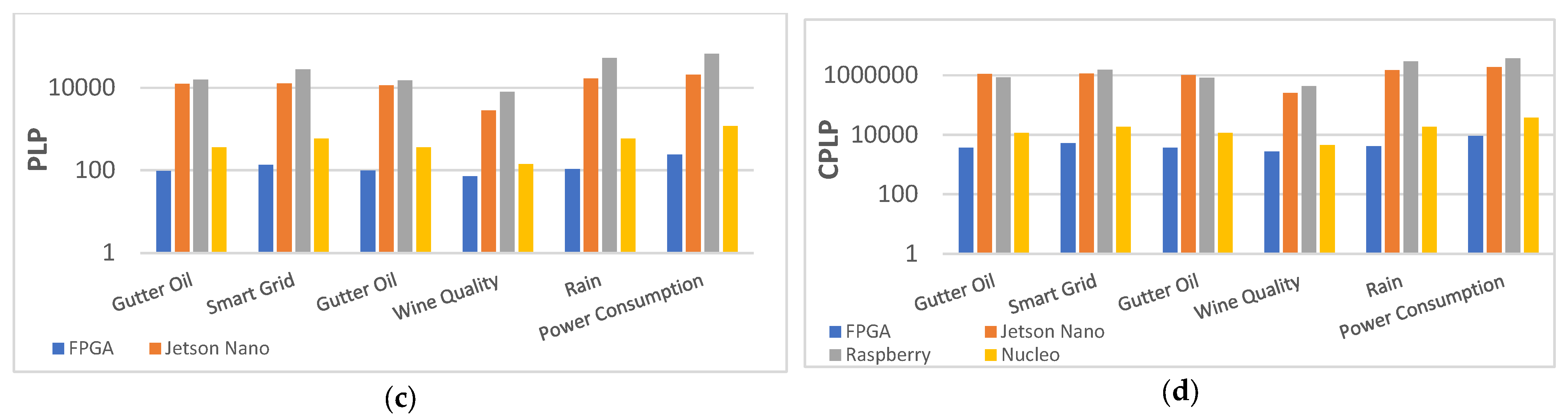As shown in Table 5, part of the EDAs is integrated with synthesis tools, such as Gowin and Pango. However, as Synplify requires an individual supporting license, in this paper, only their self-developed synthesis tools (GowinSynthesis, ADS) are used for analyzing FPGA implementations. The analysis of FPGA implementations is not limited to the computing performance, but encompasses all aspects of the hardware. While Power Latency Production (PLP) [38] is a common metric for evaluating the results of FPGA implementations, it does not consider the cost, which is a critical factor in IoT endpoint device development. As a result, we introduce the Cost Power Latency Production (CPLP) as an additional metric for evaluating the results.

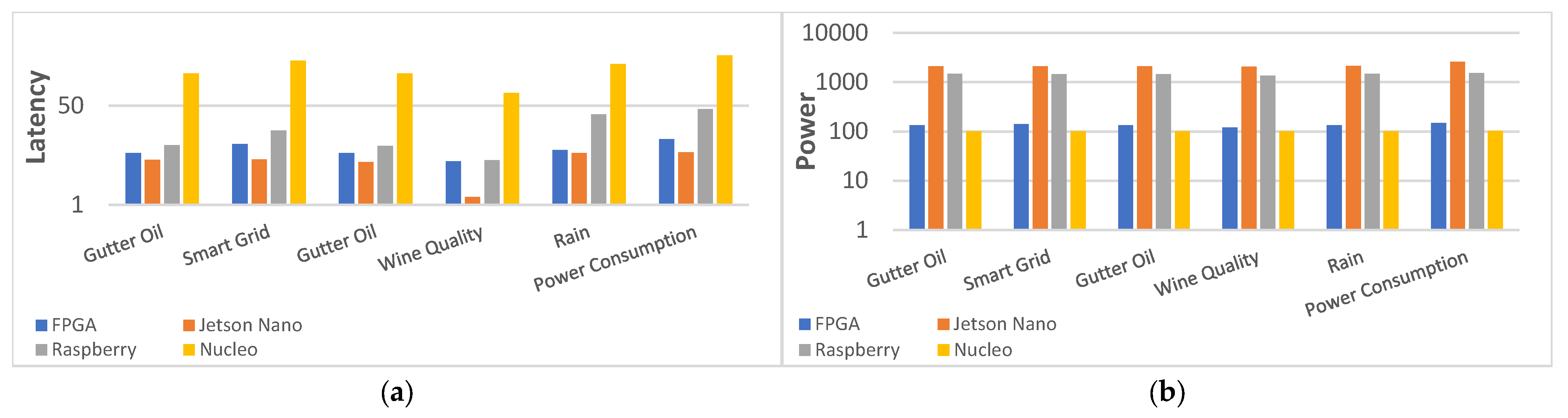
In addition, we realize the same machine learning algorithms and parameters to the Nvidia Jetson Nano 2, the Raspberry Pi 3B+, and STM32L476 Nucleo, respectively [39], allowing for more comprehensive comparisons of the implementations within different FPGAs.

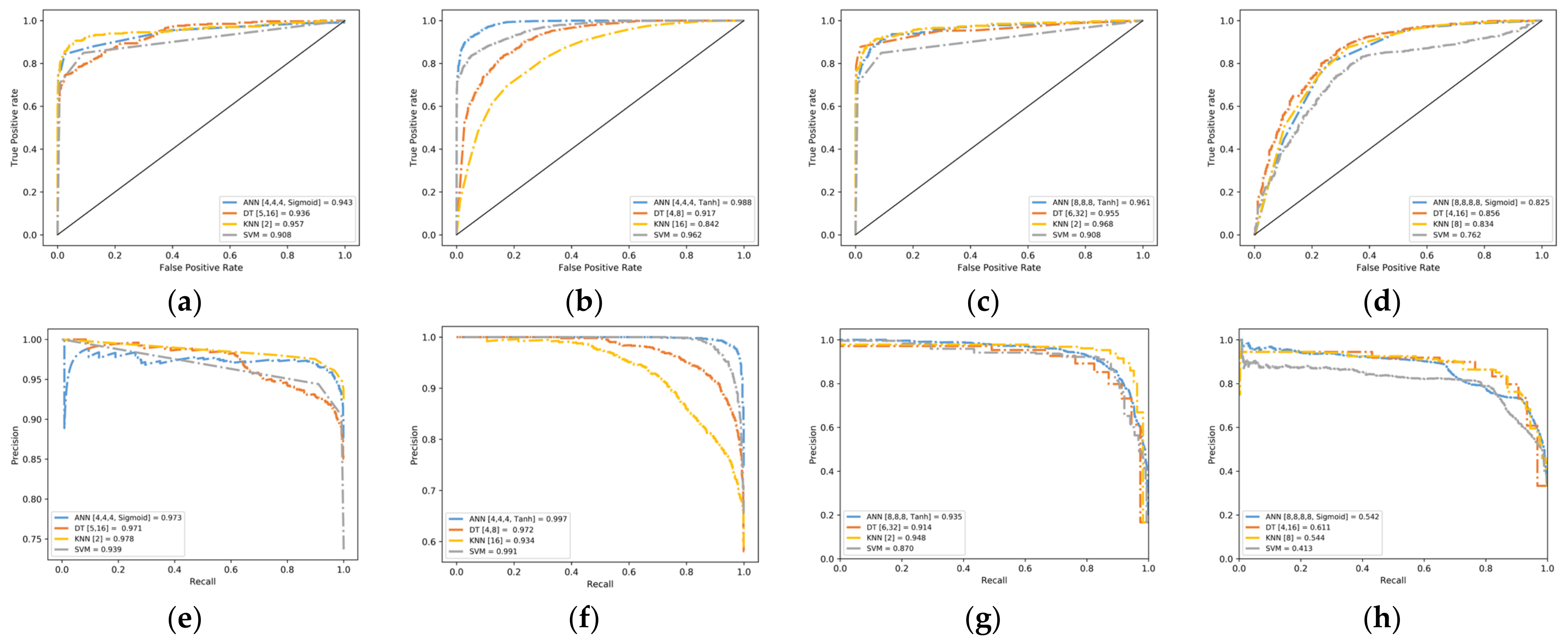
5.1. ANN

5.1.1. ANN Parameter Analysis

We intend to find the best user-defined ANN parameters in six datasets, including the number of hidden layers, neurons within each layer, and activation functions. Different combinations of these parameters are used to train our ANN model on the desktop PC and their corresponding results are shown in Appendix A, Table A1. There are only minor differences among all the combinations. We chose to apply parameters with the best score from the software to our hardware implementation. The hyperparameter values associated with the best scores for these datasets processed using the ANN algorithm are shown in Table 7.

Table 7. The highest-scoring parameters of ANN obtained in different datasets.

Dataset		Score	ANN Architectures	Activation Function
Binary classification	Gutter Oil	97.14%	[4,4,4]	Sigmoid
	Smart Grid	98.73%	[4,4,4]	Tanh
Multiclass classification	Gutter Oil	97.09%	[8,8,8]	Tanh
	Wine Quality	73.01%	[8,8,8,8]	Sigmoid
Regression	Rain	0.8583 (R2)	[8,8,8,8]	ReLU
	Power Consumption	0.9979 (R2)	[8,8]	Sigmoid

5.1.2. Implementation and Analysis of ANN Hardware

Based on the ANN architectures in Table 7, we use the corresponding EDA (with the Balanced Optimization Mode in Synthesis Settings) to implement ANN on 10 different FPGA boards. The results are summarized in Appendix A, Table A2. In terms of computing performance (latency), Intel MAX10M50DAF outperforms the others in five out of six datasets, while PGL12G outperforms the competition in the Rain task. The performance differences in time delay between 10 FPGAs are all at the millisecond level, which can almost be ignored. For the comprehensive comparisons, Lattice’s ICE40UP5 has achieved first place in most application scenarios for its extremely low power consumption and cost-effectiveness among most of the datasets (five out of six). One exception is that in the Wine Quality task scenario, it was not implemented on ICE40UP5 due to the resource constraint. In addition, the device that performed the best on the Wine Quality task was Lattice MachXO2. The FPGA deployment results with the best comprehensive performance under each task are shown in Table 8.

Table 8. ANN deployment results on the best CPLP-performing FPGAs.

Dataset		Device	Score	LUTs	DSPs	Latency/us	Power/mW	PLP	CPLP
Binary classification	Gutter Oil	ICE40UP5	97.14%	1898	8	11.12	140	1556.10	59,131.80
	Smart Grid	ICE40UP5	98.73%	1855	8	11.12	140	1556.10	59,131.80
Multiclass classification	Gutter Oil	ICE40UP5	97.09%	3887	8	11	140	1540	58,520
	Wine Quality	MachXO2	73.01%	6114	/	12.73	192	2444.54	73,091.87
Regression	Rain	ICE40UP5	0.8583 (R2)	3553	8	8.73	135	1178.69	44,790.03
	Power Consumption	ICE40UP5	0.9979 (R2)	3653	8	11.98	140	1676.50	63,707

5.2. DT

5.2.1. Analysis of DT Parameters

For PC simulations, 12 different combinations of the maximum depth and the maximum number of leaf nodes are chosen. The results are shown in Appendix A, Table A3. Different DT structures produce nearly identical results. Adding the maximum depth and the maximum number of leaf nodes has no significant improvement on the score. Here, we chose the best results from various combinations for hardware deployment, and the results with the best scores for the six datasets are shown in Table 9.

Table 9. The highest-scoring parameters of DT obtained in different datasets.

Dataset		Score	Max Depth	Max Leaf Nodes
Binary classification	Gutter Oil	96.18%	5	16
	Smart Grid	97.98%	4	8
Multiclass classification	Gutter Oil	96.85%	6	32
	Wine Quality	83.69%	4	16
Regression	Rain	0.8481 (R2)	4	8
	Power Consumption	0.9976 (R2)	6	64

5.2.2. Implementation and Analysis of DT Hardware

Based on the DT architectures in Appendix A, Table A4, we use the appropriate EDA (with the Balanced Optimization Mode in Synthesis Settings) to implement DT on 10 different FPGA boards. In terms of computing performance, Intel MAX10M50DAF outperforms the competition in all six datasets. While in terms of comprehensiveness, Lattice’s ICE40UP5 came to first place again in most application scenarios for its extremely low power consumption and cost-effectiveness. The FPGA DT deployment results with the best comprehensive performance under each task are shown in Table 10.

Table 10. DT deployment results on the best CPLP-performing FPGAs.

Dataset		Device	Score	LUTs	DSPs	Latency/us	Power/mW	PLP	CPLP
Binary classification	Gutter Oil	ICE40UP5	96.18%	451	0	7.92	133.90	1060.76	3882.38
	Smart Grid	ICE40UP5	97.98%	285	0	5.87	122	716.14	2873.01
Multiclass classification	Gutter Oil	ICE40UP5	96.85%	715	0	7.92	135	1069.47	3876.36
	Wine Quality	ICE40UP5	83.69%	305	0	5.60	121	677	2740.86
Regression	Rain	ICE40UP5	0.8481 (R2)	303	0	5.80	121	701.80	2838.75
	Power Consumption	ICE40UP5	0.9976 (R2)	765	0	9.65	128	1235.46	4723.10

5.3. K-NN

5.3.1. Analysis of k-NN Parameters

In our k-NN model, the parameter k is user-defined. We experiment with various k values when training our model on the PC, and the results are shown in Appendix A, Table A5. The increment of k has no significant effect on the score. In fact, on the contrary, it might decrease them. We deploy the architecture that is optimal in terms of k value for hardware deployment. The hyperparameter values associated with the best scores for these datasets processed using the k-NN algorithm are shown in Table 11.

Table 11. The highest-scoring parameters of k-NN obtained in different datasets.

Dataset		Score	k Values
Binary classification	Gutter Oil	99.36%	2
	Smart Grid	79.39%	16
Multiclass classification	Gutter Oil	99.36%	2
	Wine Quality	81.23%	8
Regression	Rain	0.8527 (R2)	16
	Power Consumption	0.9960 (R2)	2

5.3.2. Implementation and Analysis of k-NN

According to the k parameters analyzed in Section 5.3.1, we implement our model on 10 FPGA boards (with the Balanced Optimization Mode in Synthesis Settings). The corresponding results are shown in Appendix A, Table A6. Gowin’s GW2A has the best computing performance in all of the task scenarios. By relying on extremely low power consumption and cost-effectiveness, Lattice’s ICE40UP5 achieves the best comprehensive performance across all datasets.

Additionally, two things are worth noting: Anlogic’s EF2M45 and Lattice’s MachXO2 are unable to deploy k-NN in multiple mission scenarios due to resource constraints. Pango’s PGL12G is also incapable of deploying k-NN. In addition, the reason is that the synthesis tool is unable to correctly recognize the current k-NN design, and therefore ignores the key path. This does not occur when using alternative development tools. The FPGA k-NN deployment results with the best comprehensive performance under each task are shown in Table 12.

Table 12. The k-NN deployment results on the best CPLP-performing FPGAs.

Dataset		Device	Score	LUTs	DSPs	Latency/us	Power/mW	PLP	CPLP
Binary classification	Gutter Oil	ICE40UP5	99.36%	979	6	7.81	134	1046.54	39,768.52
	Smart Grid	ICE40UP5	79.39%	4949	8	9.32	135.79	1265.58	48,092.09
Multiclass classification	Gutter Oil	ICE40UP5	99.36%	1077	6	7.81	135	1054.35	40,065.30
	Wine Quality	MachXO2	81.23%	4348	/	7.18	186	1335.67	39,936.41
Regression	Rain	Cyclone10LP10CL	0.8527 (R2)	5397	8	11.89	305.54	3633.79	181,325.98
	Power Consumption	ICE40UP5	0.9960 (R2)	1159	7	9.36	12.71	118.97	4520.69

5.4. SVM

In the experiment, the linear SVM is chosen for training, and the results are shown in Table 13. Due to the function similarity between the linear SVM and ANN, their simulation scores are very similar. The SVM deployment results on 10 FPGA boards with the best comprehensive performance under each task are shown in Table 14. The remaining implementation results are provided in the Appendix A, Table A7.

Table 13. The highest-scoring of SVM obtained in different datasets.

Dataset		Score
Binary classification	Gutter Oil	96.02%
	Smart Grid	98.35%
Multiclass classification	Gutter Oil	96.33%
	Wine Quality	72.68%
Regression	Rain	0.7932 (R2)
	Power Consumption	0.9979 (R2)

Table 14. SVM deployment results on the best CPLP-performing FPGAs.

Dataset		Device	Score	LUTs	DSPs	Latency	Power	PLP	CPLP
Binary classification	Gutter Oil	ICE40UP5	96.02%	765	8	15.56	151	2349.41	89,277.54
	Smart Grid	ICE40UP5	98.35%	955	8	15.90	154.98	2464.17	93,638.31
Multiclass classification	Gutter Oil	ICE40UP5	96.33%	765	8	14.90	152.99	2279.20	86,609.61
	Wine Quality	ICE40UP5	72.68%	976	8	15.56	155.14	2413.89	91,727.65
Regression	Rain	ICE40UP5	0.7932 (R2)	527	8	13.51	147.76	1996.77	75,877.43
	Power Consumption	ICE40UP5	0.9979 (R2)	516	8	13.47	148	1994.00	75,772.15

5.5. Comparisons with Embedded Platforms

To provide a more accurate assessment of our implementation, we also compare MLoF with three representative embedded platforms, namely Nvidia Jetson Nano, Raspberry Pi3 B+, and STM32L476 Nucleo. The specification of each platform is listed in Table 15. Jetson Nano is powered by a Cortex-A57 core running at 1.43 GHz and a 128-core Nvidia Maxwell-based GPU [40], while Raspberry features a Cortex-A53 core running at 1.2 GHz. STM32L476 Nucleo is a typical IoT development platform with a Cortex-M4 core running at 80 MHz [41]. Compared with Table 4, the prices of these three representative embedded development platforms are similar to the FPGAs, which indicates that all of them are comparable in terms of other indexes. Given the proper cost of FPGAs, they can be considered as competitive substitutes for past typical platforms.

Table 15. The specification of three representative embedded development platforms.

Platform	Processor	Clock	Price
Nvidia Jetson Nano	Cortex-A57	1.43 GHz	$89.00
Raspberry Pi3 B+	Cortex-A53	1.2 GHz	$54.99
STM32L476 Nucleo	Cortex-M4	80 MHz	$31.99

Based on the simulation results of previous desktop PCs, the Receiver Operating Characteristic (ROC) curve and Precision-Recall (PR) curve shown in Figure 10, we select the models with the highest score in each of the six task scenarios for deployment of the embedded platform [42]. The corresponding deployment models and architectures for each task are listed in Table 16. PyCuda is used for GPU parallel acceleration with fixed weight parameters on Jetson Nano. Moreover, we use the same Python code to implement it on the Raspberry Pi, as well.

Figure 10. Comparison of the receiver operating characteristic curve and precision-recall curve for the six typical IoT endpoint datasets with different algorithms. (a) Receiver Operating Characteristic curve for Gutter Oil binary classification; (b) Receiver Operating Characteristic curve for Smart Grid binary classification; (c) Receiver Operating Characteristic curve for Gutter Oil multiclass classification; (d) Receiver Operating Characteristic curve for Smart Grid multiclass classification; (e) Precision-Recall curve for Gutter Oil binary classification; (f) Precision-Recall curve for Smart Grid binary classification; (g) Precision-Recall curve for Gutter Oil multiclass classification; (h) Precision-Recall curve for Smart Grid multiclass classification.

Table 16. The highest-scoring model obtained in different datasets.

Dataset		Model	Score	Architecture
Binary classification	Gutter Oil	k-NN	99.36%	K = 2
	Smart Grid	ANN	98.73%	[4,4,4], Tanh
Multiclass classification	Gutter Oil	k-NN	99.36%	K = 2
	Wine Quality	DT	83.69%	Max depth = 4, Max node = 16
Regression	Rain	ANN	0.8583 (R2)	[8,8,8], ReLU
	Power Consumption	SVM	0.9979 (R2)	N/A

Table 17 compares the performance of our FPGA and three embedded platform implementations. Jetson Nano takes the lead in terms of computing performance. On the other hand, Nucleo consumes the lowest power. While the power consumption of FPGA decreased by an average of 891%, and its performance improved by an average of 9 times compared to typical IoT endpoint platforms. Moreover, FPGAs outperform all other platforms in terms of Energy Efficiency (PLP) and Cost Efficiency (CPLP).

Table 17. Breakdown of platform implemented results.

Dataset and Type of Module			The Best of FPGA	Jetson Nano	Raspberry	Nucleo
Binary classification	Gutter Oil (k-NN)	Accuracy	99.36%	99.36%	99.36%	99.36%
		Latency	7.81 us	5.90 us	10.51 us	180.00 us
		Power	134 mW	2120 mW	1480 mW	102 mW
		PLP	1046.54	12,508	15,554.8	18,360
		CPLP	39,768.52	1,113,212	855,358.5	587,336.4
	Smart Grid (ANN)	Accuracy	98.73%	98.73%	98.73%	98.73%
		Latency	11.12 us	5.97 us	18.77 us	300.00 us
		Power	140 mW	2110 mW	1470 mW	101 mW
		PLP	1556.8	12,596.7	27,591.9	30,300
		CPLP	59,158.4	1,121,106	1,517,279	969,297
Multiclass classification	Gutter Oil (k-NN)	Accuracy	99.36%	99.36%	99.36%	99.36%
		Latency	7.81 us	5.44 us	10.25 us	180.00 us
		Power	135 mW	2120 mW	1470 mW	102 mW
		PLP	1054.35	11,532.8	15,067.5	18,360
		CPLP	40,065.3	1,026,419	828,561.8	587,336.4
	Wine Quality (DT)	Accuracy	83.69%	83.69%	83.69%	83.69%
		Latency	5.60 us	1.37 us	5.82 us	84.00 us
		Power	121 mW	2060 mW	1350 mW	101 mW
		PLP	677.6	2822.2	7857	8484
		CPLP	25,748.8	251,175.8	432,056.4	271,403.2
Regression	Rain (ANN)	R2	0.8583	0.8583	0.8583	0.8583
		Latency	8.73 us	7.81 us	35.77 us	261.00 us
		Power	135 mW	2140 mW	1480 mW	102 mW
		PLP	1178.55	16,713.4	52,939.6	26,622
		CPLP	44,784.9	1,487,493	2,911,149	851,637.8
	Power Consumption (SVM)	R2	0.9979	0.9979	0.9979	0.9979
		Latency	13.47 us	7.94 us	43.73 us	364.00 us
		Power	148 mW	2610 mW	1530 mW	103 mW
		PLP	1993.56	20,723.4	66,906.9	37,492
		CPLP	75,755.28	1,844,383	3,679,210	1,199,369

To demonstrate the benefits of FPGA implementation in IoT endpoint scenarios, we compare embedded and FPGA platforms using six datasets in terms of performance (latency), power consumption, PLP, and CPLP, as shown in Figure 11 with the ordinate-axis in logarithmic scale. Jetson Nano exceeds the others in performance, but the second-best FPGA is not far behind, only 38% lower in average, 100% ahead of Raspberry, and 2300% ahead of Nucleo. In terms of power consumption, Nucleo is quite competitive as a low-power MCU with 102 mW on average, 30 mW lower than FPGA. These two platforms advanced well beyond Jetson Nano and Raspberry. It can be clearly seen that in comparison to other platforms, FPGAs require significantly less PLP and CPLP on the ordinate-axis in logarithmic scale. The smallest PLP and CPLP are critical for IoT endpoint development and implementation, as response time, power consumption, and cost are all critical factors in IoT endpoint tasks. Furthermore, the FPGA PLP is 17× better than the average for embedded platforms and the FPGA CPLP is 25× better than the average for embedded platforms.

Figure 11. Comparison of performance (latency), power consumption, PLP, and CPLP for the six typical IoT endpoint datasets with different algorithms when implemented on FPGA and embedded platforms. (a) Comparison of performance (latency). (b) Comparison of power consumption. (c) Comparison of PLP. (d) Comparison of CPLP.

6. Conclusions

In this paper, the Machine Learning on FPGA (MLoF), a series of ML hardware accelerator IP cores for IoT endpoint devices was introduced to offer high-performance, low-cost, and low-power.

MLoF completes the process of making inferences on FPGAs based on the optimal parameter results from PC training. It implements four typical machine learning algorithms (ANN, DT, k-NN, and SVM) with Verilog HDL on 10 FPGA development boards from seven different manufacturers. The usage of LUTs, Power, Latency, Cost, PLP, as well as CPLP are used in comparisons and analyses of the MLoF deployment results with six typical IoT datasets. At the same time, we analyzed the synthesis results of different EDA tools under the same hardware design. Finally, we compared the best FPGA deployment results with typical IoT endpoint platforms (Jetson Nano, Raspberry, STM32L476). The results indicate that the FPGA PLP outperforms the IoT platforms by an average of 17× due to their superior parallelism capability. Meanwhile, FPGAs have 25× better CPLP compared to the IoT platforms. To our knowledge, this is the first paper that conducts hardware deployment, platform comparisons, and deployment result analysis. At the same time, it is also the first set of IP on open-source FPGA machine learning algorithms, and has been verified on low-cost FPGA platforms.

MLoF still has room for further improvements: 1. The adaptability of MLoF could be enhanced, thus more complex algorithms (kNN with k > 16) could also be deployed on low-cost FPGAs with few resources, such as MachXO2; 2. More options for user parameters configuration could be added, including more ML algorithms, larger data bit width, and more hyperparameters; 3. Usability could be improved by further providing a script file or a user interface, to help the users generate the desired ML algorithm IP core more easily. These existing shortcomings of MLoF point out the direction of our future work.