Evaluation of Real-Time Kinematic Positioning and Deformation Monitoring Using Xiaomi Mi 8 Smartphone

Abstract

Modern low-cost electronic devices can achieve high precision for global navigation satellite systems (GNSSs) and related applications. Recently, the pseudo-range and carrier phase have been directly obtained from a smartphone to establish a professional-level surveying device. Although promising results have been obtained by linking to an external GNSS antenna, the real-time kinematic (RTK) positioning performance requires further improvement when using the embedded smartphone antenna. We first investigate the observation quality characteristics of the Xiaomi Mi 8 smartphone. The carrier-to-noise-density ratio of L5/E5a signals is below that of L1/E1 signals, and the cycle slip and loss of lock are severe, especially for L5/E5a signals. Therefore, we use an improved stochastic model and ambiguity-resolution strategies to improve the short-baseline RTK positioning accuracy. Experimental results show that the ambiguity fixing rate can reach approximately 90% in 3 h of observations when using the embedded antenna, while the GPS/Galileo/BDS single-frequency combination is more suitable for smartphones. On the other hand, convergence takes 10–30 min, and the RTK positioning accuracy can reach 1 and 2 cm along the horizontal and vertical directions, respectively, if ambiguity is resolved correctly. Moreover, we verify the feasibility of using a mass-produced smartphone for deformation monitoring. Results from a simulated dynamic deformation experiment indicate that a smartphone can recognise deformations as small as 2 cm.

1. Introduction

With the development of satellite navigation and positioning technologies, users’ demand for global navigation satellite system (GNSS) equipment with accurate positioning has steadily increased. Thus, developing high-precision applications based on low-cost GNSS equipment has become a dominant trend. Smartphones are one of the most used low-cost GNSS devices, accounting for 80% of the total number of GNSS devices available worldwide [1]. Compared with professional GNSS equipment, a smartphone has small size, low cost, and ease of use. However, the main shortcoming of the smartphone GNSS module is its poor positioning accuracy, with the standard single-point positioning precision being typically approximately 10 m on the horizontal plane [2], greatly limiting its use for professional applications.

Research on smartphone GNSS modules has been conducted for many years, but before 2016, users could only obtain position, velocity, time, altitude, azimuth, and other final positioning information from a smartphone [3], thus restricting the development of smartphone GNSS technology. In May 2016, Google opened the GNSS raw measurement application programming interface for smartphones in the Android Nougat (version 7.0) operating system [4]. Since then, users can directly access observations including pseudo-range, carrier phase, and Doppler observable from a smartphone. Such data accessibility has greatly contributed to the development of high-precision smartphone GNSS modules toward positioning at the decimetre level or even the centimetre level, thus expanding their adoption in the GNSS market.

Broadcom launched a dual-frequency GNSS chip, and Xiaomi Mi 8 was the world’s first smartphone with a dual-frequency GNSS function. Thereafter, smartphones equipped with chips made in China, such as Huawei P40 and Huawei Mate40, have integrated tri-frequency and quad-frequency GNSS functions. Currently, many smartphones are endowed with multi-constellation and multi-frequency capabilities, and their signal volume is comparable to that of survey-grade receivers, likely enabling high-precision positioning.

By leveraging the aforementioned advances, many studies have been conducted on smartphone GNSS raw measurements, aiming to comprehensively analyse the observation quality and positioning performance of various smartphones and implement high-precision applications. However, owing to the embedded low-cost antenna and chip, smartphone GNSS modules present many problems. Typically, the carrier-to-noise-density ratio (C/N0) of a smartphone is approximately 10 dB-Hz lower than that of a geodetic receiver, and it is more sensitive to multipath interference [5]. In addition, the correlation of the observation quality with C/N0 is stronger than that with the elevation [6], and the pseudo-range noise of a smartphone is approximately 10 times larger than that of a geodetic receiver. Moreover, the carrier-phase noise is approximately 3–5 times larger than that of a geodetic receiver [7], and it is sensitive to the duty cycle mechanism [6,8]. Consequently, the carrier phase presents frequent cycle slips and continuous loss of lock. Although these observation problems greatly limit accuracy, high-precision positioning at the centimetre level is still achievable in smartphones [5].

Technologies such as precise point positioning, real-time kinematic (RTK) positioning, and network RTK positioning have been used to develop high-precision applications for smartphones. Realini et al. [9] used GNSS raw measurements from smartphones for positioning tests, achieving decimetre-level accuracy through relative positioning. Dabove et al. [10] equipped both a base station and a rover with smartphones, achieving decimetre-level RTK positioning accuracy and centimetre-level repeatability. Zhang et al. [5] implemented a method for precise point positioning based on the time-difference carrier phase using a Nexus 9 smart device achieving sub-metre-level positioning accuracy. Dabove et al. [11] also studied the performance of a smartphone using network RTK positioning with differential correction observations from the Continuously Operating Reference Stations, achieving centimetre-level precision but only decimetre-level accuracy. They found that to improve decimetre-level accuracy in smartphones, the integer ambiguity should be resolved.

A correct and reliable ambiguity-fixed solution can lead to centimetre-level positioning accuracy [12], even in smartphones. Wanninger et al. [13] conducted experiments on a Huawei P30 smartphone, and the results showed that only the GPS (global positioning system) L1 signal can resolve ambiguity. Geng et al. [14] attached an external survey-grade GNSS antenna to a smartphone, achieving a fixed solution, while Bochkati et al. [15] used a choke-ring to reduce multipath interference, obtaining an ambiguity fixing rate up to 89% and RTK positioning accuracy of 1–2 cm. Gao et al. [16] also used a survey-grade antenna to resolve ambiguity in RTK positioning, achieving 100% fixing rate and millimetre-level positioning accuracy. These methods have demonstrated the ability of GNSS modules in smartphones to achieve high-precision positioning. However, applicability may be reduced by using an external GNSS antenna or a choke-ring on a smartphone because it increases the equipment burden for surveying. In addition, the signal reception of the built-in smartphone antenna should be shielded to prevent interference from the external antenna. Despite the difficulty in achieving high-precision positioning using only the internal smartphone antenna, further optimisation in the underlying algorithms may improve the positioning performance.

Regarding practical applications, Uradziński et al. [17] found that smartphones can achieve centimetre-level accuracy when ambiguity is resolved, enabling geodetic and monitoring applications. Julián et al. [18] used smartphones in forestry surveys, finding that the high sensitivity of smartphones is advantageous for forest sheltered environments, but the positioning accuracy should be further improved. These applications illustrate the importance of high-precision positioning in smartphones. Although the current accuracy has certain bottlenecks, high-performance positioning would be of great significance to many users.

Our Contribution

To fully exploit the advantages of smartphone multi-GNSS signals, namely low cost and ease of use, in this paper, we propose the application of smartphones to dynamic deformation monitoring. This would broaden the application field of smartphones and promote the application of low-cost receivers in deformation monitoring. To achieve this goal, we focused on solving the problem of ambiguity, which is difficult to resolve when using the internal smartphone antenna, through data processing. In the first part of the study, the quality characteristics of dual-frequency observations acquired from a Xiaomi Mi 8 smartphone are analysed. Then, we propose an improved dual-frequency stochastic model based on the quality characteristics, combined with a partial ambiguity resolution algorithm [19] to increase the ambiguity fixing rate and positioning accuracy. Subsequently, the ambiguity resolution performance of short-baseline RTK is analysed. Finally, considering fixed ambiguity, the feasibility of using a mass-produced smartphone for deformation monitoring is evaluated.

2. Smartphone Global Navigation Satellite System (GNSS) Data Collection and Analysis

We collected smartphone GNSS data in a real environment and analysed their quality.

2.1. Data Collection

Data collection experiments were conducted on the rooftop of an office building in Central South University, China. We adopted the short-baseline static mode, which is approximately 5 m for the baseline length. The reference station was equipped with a survey-grade antenna (TRM 57971.00) and a geodetic receiver (Trimble Net R9), and the rover station was a Xiaomi Mi 8 smartphone running the Android 9.0 operating system. This smartphone supports five constellations with dual-frequency signals (i.e., GPS L1/L5, GLONASS G1, BDS B1, Galileo E1/E5a, and QZSS L1/L5), and its duty cycle [6], which is a battery-saving mechanism in the smartphone GNSS module, can be turned off. In this study, we disregarded the QZSS constellation. To obtain the smartphone GNSS observation data for analysing and solving the data in post time, we used the Geo++ RINEX Logger (v2.1.3) [20] Android mobile application. During measurement, users only need to turn on the “Dual GPS” positioning function and click start logging to start recording the observation data. The application automatically stores the GNSS data in RINEX format, which is convenient for users to directly process GNSS data. Approximately 5 h of data were collected on 15 November 2020 at a sampling interval of 1 s. The first 3 h was used for analysis, and the results of the last 2 h were consistent with the results of the first 3h, so we do not use the last 2 h to reduce the calculation time. It is considered that the sampling rate of 1 Hz is high enough; hence, 3 h is sufficient to guarantee the required amount of data.

Although mobile phone manufacturers do not publish the location of the smartphone GNSS antenna, Netthonglang et al. [21] estimated the antenna position of Xiaomi Mi 8 through relative positioning with centimetre-level accuracy. The antenna phase centre is on the left side of the front of the phone (Figure 1). To facilitate centring, we used the top centre of the smartphone as the antenna reference point (ARP), whose distance from the phase centre is shown in Figure 1.

Figure 1. Diagram of global navigation satellite system (GNSS) antenna phase centre in Xiaomi Mi 8 smartphone [21].

The fixed control point (FCP) shown in Figure 2 was used as reference, and its accurate coordinates were obtained using two geodetic receivers through relative positioning. To ensure full GNSS signal reception, we placed the smartphone vertically using a holder. The FCP was taken as the centring point, and the centring accuracy was within 1 cm. We measured the distance between the smartphone ARP and the FCP along three directions (i.e., east, north, and up) and the angle between the orientation perpendicular to the screen and the true north (28.0°). Hence, we calculated the offset along the east, north, and up directions to obtain the overall phase centre offset provided in Table 1.

Figure 2. Fixed control point (FCP) and equipment placement.

Table 1. Offset of smartphone antenna phase centre with respect to FCP.

East (m)	North (m)	Up (m)
−0.027	−0.015	+0.191

2.2. Data Quality Analysis

We analysed the dual-frequency GNSS observations collected in the experiment to obtain a reference for data processing during positioning. The statistical results reported below exclude data with elevations below 10°.

2.2.1. Dual-Frequency C/N0 Analysis

C/N0 is an important data quality indicator for GNSS, and it is related to the receiver hardware and signal path [5]. Figure 3 shows the C/N0 sequence and statistical results of the different types of observations. The maximum C/N0 is below 50 dB-Hz. The L1/G1/B1/E1 signals are mainly concentrated around 40 dB-Hz, but some satellites provide signals below 20 dB-Hz, while the Galileo satellites provide signals above 30 dB-Hz. The GPS L5, Galileo E1/E5a, and BDS GEO satellites were slightly stable during measurement, while other satellites fluctuated greatly. Overall, Galileo satellites provide the highest signal stability and strength, but their number is low.

Figure 3. C/N0 of different types of observations. (a) C/N0 sequence. (b) Statistical results of mean C/N0.

For band L5/E5a, C/N0 is mainly concentrated at 30 dB-Hz, being lower than the mean C/N0 for band L1/G1/B1/E1. The L5/E5a multipath resistance is stronger in smartphones [8,22], and the signal quality is usually better than that in band L1/E1. However, in our results, the C/N0 of band L5/E5a is lower. Therefore, when establishing a stochastic model for multi-frequency observations, the difference in multi-frequency C/N0 should be considered.

2.2.2. Dual-Frequency Cycle Slip Analysis

Cycle slip is an important indicator of carrier-phase quality. Figure 4 shows the time sequence diagram of satellite visibility and its cycle slip for the four constellations, and Figure 5 shows the statistical results of cycle slips. Each cycle slip is marked with a red plus sign, and it is mainly determined by the loss-of-lock indicator, which may also reflect carrier-phase interruption.

Figure 4. Satellite visibility and cycle slips (red plus signs) of four constellations on two frequency bands: (a) global positioning system (GPS) L1/GLONASS G1/Galileo E1/BDS B1; (b) GPS L5/Galileo E5a. (PRN, pseudorandom noise).

Figure 5. Statistical results of cycle slips for four constellations. (a) Ratio of cycle slips to number of observations. (b) Ratio of cycle slips to number of cycle slips in various C/N0 ranges.

Figure 4 shows several satellites observed during the entire period, with reception from 34 satellites overall, including 11 GPS, 9 GLONASS, 5 BDS, and 9 Galileo satellites. In addition, seven GPS satellites deliver L5 signals, and five Galileo satellites deliver E5a signals. The cycle slips or interrupts are frequent, especially for L5/E5a signals. In terms of statistical results, for the first frequency band (L1/G1/B1/E1), the cycle slips of BDS are comparatively more frequent, while almost no slip occurs for the Galileo satellites. However, the cycle slips of GPS L5 and Galileo E5a signals are severe, accounting for more than 5%, which is much higher than the rate for L1/E1 signals. These results show that band L5/E5a is more prone to cycle slip. In addition, the number of satellites delivering signals in this frequency band is low, further reducing the availability of dual-frequency observations in smartphones.

From the statistical results of cycle slips for different C/N0 ranges (Figure 5b), 90.6% of the cycle slips in band L1 are mainly concentrated in the range below 35 dB-Hz, and 99.0% of the cycle slips in band L5 are concentrated in the range below 30 dB-Hz. Overall, the cycle slips are highly severe when C/N0 is lower than 30 dB-Hz. Therefore, the C/N0 threshold should be set to prevent low-quality observations from participating in data processing or ambiguity resolution.

3. Data Processing and Analysis for Smartphone Real-Time Kinematic (RTK) Positioning

RTK positioning is a widely used high-precision technology in GNSS. As it can eliminate most of the external system errors, RTK positioning can enable high-precision applications in smartphones. In RTK positioning, we apply the double-difference method to both pseudo-range and carrier phase observations to eliminate observation errors. First, single-difference observations are obtained by the difference between observations from rover station $r_1$ and reference station $r_2$. The obtained single-difference observations are differenced by satellites $i$ and $j$ (reference) to calculate the double-difference observations. In short baselines, the double difference can eliminate satellite-orbit and clock errors, receiver-clock errors, ionospheric and tropospheric delays, and other errors, leaving mainly multipath and measurement noise. When the multipath is significant, the observations for low-cost receivers may be correlated. Therefore, in this study, we first minimize the multipath from the source of data collection and then use a C/N0 stochastic model to reduce the impact of multipath. Hence, it is assumed that the remaining error is random. Under this condition, the double-difference observation equation is given by [23]:

$$P_{ij}^{r_1{r}_2}={\rho }_{ij}^{r_1{r}_2}+{\epsilon }_{ij}^{r_1{r}_2},$$

(1)

$${\varphi }_{ij}^{r_1{r}_2}={\rho }_{ij}^{r_1{r}_2}+\lambda N_{ij}^{r_1{r}_2}+{\eta }_{ij}^{r_1{r}_2},$$

(2)

where the superscript and subscript represent the station difference and satellite difference, respectively, $P$ represents the pseudo-range observations, $\varphi$ represents the carrier-phase observations, $\lambda$ is the wavelength of the carrier phase, $\rho$ is the geometric distance calculated by the satellite and receiver coordinates, $N$ is the carrier-phase ambiguity, and $\epsilon$ and $\eta$ are pseudo-range and carrier-phase measurement noise terms, respectively. A more compact expression is given by:

$$y=Aa+Bb+\Delta ,$$

(3)

where $y$ represents the observation vector, $a$ represents the coordinate parameter vector, $A$ is its coefficient matrix, $b$ represents the ambiguity parameter vector, $B$ is its coefficient matrix, and $\Delta$ represents the noise vector. In RTK positioning, the Kalman filter [23] is typically used to estimate the unknown floating-point parameters. If high-quality observations $P$, observation data $\phi$, and correctly resolved ambiguity $N$ are obtained, high-precision RTK positioning is achieved.

According to the data quality analysis above, we adopt improved data quality control and integer ambiguity resolution for smartphone RTK positioning. In addition, we analyse RTK positioning for different combinations of observations and its convergence time in different periods.

3.1. Data Processing for Smartphone RTK Positioning

3.1.1. Stochastic Model and Cycle-Slip Detection

Satellite elevation is conventionally used to determine stochastic models in GNSS data processing. However, Liu et al. [6] found that the accuracy of GNSS observations in smartphones is more correlated with C/N0 than with elevation. Thus, it is more reasonable to use C/N0 to determine the stochastic model. The conventional elevation model and C/N0 model SIGMA-ε [24] are, respectively, formulated as follows:

$${\sigma }_g^2=a_0^2+\frac{b_0^2}{{\sin }^2(el)},$$

(4)

$${\sigma }_S^2=C_i\cdot {10}^{-\frac{\mathrm{CN}0}{10}},$$

(5)

where ${\sigma }_g^2$ is the observation variance for the elevation model, $el$ is the satellite elevation, $a_0$, $b_0$ and $C_i$ are model coefficients, ${\sigma }_S^2$ is the observation variance for the C/N0 model, and $\mathrm{CN}0$ is the C/N0 value.

Considering the differences in C/N0 ranges for different frequencies in the smartphone signals, if the C/N0 model is used directly, the L5/E5a frequency weight may be lower than the L1/E1 frequency weight, being contrary to the smaller noise of L5/E5a observations. Therefore, based on the C/N0 stochastic model proposed in [25], we set different thresholds for different frequencies in the model to reduce the impact of differences in dual-frequency C/N0. As the reference station is a geodetic receiver, it uses an elevation model. According to the law of error propagation, the variance of the single-difference observation should be the sum of the variances of the two stations:

$${\sigma }_{S_L}^2=\left\{\begin{array}{lll}{a}_0^2\cdot {10}^{-(\frac{\mathrm{CN}0-{\mathrm{CN}0}_{\mathrm{MAX}}}{10})}\hfill & ,\hfill & \mathrm{CN}0<{\mathrm{CN}0}_{\mathrm{MAX}}\hfill \\ a_0^2\hfill & ,\hfill & \mathrm{CN}0\ge {\mathrm{CN}0}_{\mathrm{MAX}}\hfill \end{array}\right.,$$

(6)

$${\sigma }_L{}^2={\sigma }_g^2+{\sigma }_{S_L}^2,$$

(7)

where ${\sigma }_{S_L}^2$ is the observation variance of the smartphone signals, $L$ denotes the frequency band, ${\sigma }_L{}^2$ is the variance of the single-difference observation, and ${\mathrm{CN}0}_{\mathrm{MAX}}$ is the maximum C/N0 in the corresponding band. For comparison, we set two types of ${\mathrm{CN}0}_{\mathrm{MAX}}$ values for the two frequencies: unified ${\mathrm{CN}0}_{\mathrm{MAX}}$ and individual ${\mathrm{CN}0}_{\mathrm{MAX}}$. We call the corresponding models unified-CNM model and individual-CNM model. For the unified-CNM model, ${\mathrm{CN}0}_{\mathrm{MAX}}$ is set to 40 dB-Hz for all frequencies. For the individual-CNM model, ${\mathrm{CN}0}_{\mathrm{MAX}}$ is set to 45 dB-Hz for band L1/G1/B1/E1 and 35 dB-Hz for band L5/E5a according to the statistical values reported above.

The positioning performance of the elevation model and the C/N0 models, namely, SIGMA-ε, unified-CNM, and individual-CNM, are evaluated in Section 3.2. Here, we briefly analyse the feasibility of the three C/N0 models. Taking G26 as an example, the variance ratios of bands L1 and L5 (i.e., ${\sigma }_{S_{L1}}^2/{\sigma }_{S_{L5}}^2$) for the three C/N0 models are shown in Figure 6. For the SIGMA-ε model, the observation variance in band L1 is lower than that in band L5 (factor of 0–0.4). On the other hand, the observation noise in band L1 is higher than that in band L5 for the Xiaomi Mi 8 measurements [8,22]. Therefore, the SIGMA-ε model may set counterproductive weights when using bands L1 and L5 simultaneously. For the unified-CNM model, most ratios are lower than 1, while few are higher than 1, which may not lead to optimality. For the individual-CNM model, approximately 67.2% of the ratios are higher or equal to 1, being more promising for optimisation.

Figure 6. Variance ratio of bands G26 L1 and L5 for C/N0 stochastic models.

For cycle-slip detection in data processing, we mainly use the loss-of-lock indicator, Doppler, and code-phase combination methods for joint detection. In addition, we adopt a geometry-free method for dual-frequency observations. The code-phase combination method is greatly affected by the pseudo-range noise. Thus, a larger cycle-slip threshold should be set (15 m in this study) to detect pseudo-range gross errors simultaneously. Moreover, we set the C/N0 threshold and elevation cut-off value to eliminate the observations which are severely affected by multipath interference and cycle slip. The specifications for RTK positioning are listed in Table 2.

Table 2. Parameter settings for real-time kinematic (RTK) positioning.

Parameter	Value
Mode	Kinematic
Cut-off elevation	10°
C/N0 threshold	20 dB-Hz
Stochastic model	elevation + C/N0
	Carrier-phase noise $(a_0$$,b_0$): 0.003 m
	Code-carrier error ratio: 300:1
Cycle-slip detection	Loss-of-lock indicator/Doppler/code-carrier combination
Ambiguity resolution mode	Continuous/fix-and-hold + partial ambiguity resolution
Minimum lock to fix ambiguity	5
C/N0 threshold to fix ambiguity	30 dB-Hz
Ratio threshold to fix ambiguity	3.0

3.1.2. Partial Ambiguity Resolution

Parameter estimation allows the coordinates (i.e., baseline vector), the ambiguity floating-point solution, and its covariance matrix to be obtained. Then, the integer value of the float ambiguity must be determined to obtain the fixed-coordinate solution with resolved ambiguity. Correct ambiguity resolution is the basis for centimetre-level positioning accuracy [12]. However, the carrier phase acquired by a smartphone is noisy and sensitive to cycle slips, and the float ambiguity shows a poor integer solution [26]. When using the conventional method to fix all the float ambiguities, it may be difficult to pass the ratio test, resulting in the failure of ambiguity resolution. Hence, we only select the part of float ambiguities that have higher accuracy for resolution to improve both the fixing rate and positioning accuracy. This algorithm is called partial ambiguity resolution [19] and is described below.

First, we use the least-squares method or a Kalman filter to obtain float baseline $\widehat{a}$ and ambiguity solutions $\widehat{b}$, resulting in the following variance-covariance matrix:

$$Q=\left[\begin{array}{cc}{Q}_{\widehat{a}}& Q_{\widehat{a}\widehat{b}}\\ Q_{\widehat{b}\widehat{a}}& Q_{\widehat{b}}\end{array}\right],$$

(8)

where $Q_{\widehat{a}}$ is the variance matrix of $\widehat{a}$, $Q_{\widehat{b}}$ is the variance matrix of $\widehat{b}$, and $Q_{\widehat{a}\widehat{b}}$ and $Q_{\widehat{b}\widehat{a}}$ are the covariance matrices of $\widehat{a}$ and $\widehat{b}$.

Then, let all the ambiguity vectors be given by $\widehat{b}=[b_1,b_2,\cdots ,b_n]$ and the partial fixed-ambiguity vector be ${\widehat{b}}_p=[b_1,b_2,\cdots ,b_{ns}]$, whose variance matrix is $Q_{{\widehat{b}}_p}$. The remaining unfixed-ambiguity vector is ${\widehat{b}}_f=[b_{n-ns},b_{n-ns+1},\cdots ,b_n]$.

Next, the integer values of ${\widehat{b}}_p$ are searched using least-squares ambiguity decorrelation adjustment (LAMBDA) [27] to obtain fixed solutions ${\stackrel{⌣}{b}}_p$. The baseline solutions can be directly updated according to the correlation between the float baseline vector and fixed ambiguities (i.e., $Q_{\widehat{a}{\widehat{b}}_p}$):

$$\stackrel{⌣}{a}=\widehat{a}-Q_{\widehat{a}{\widehat{b}}_p}{Q}_{{\widehat{b}}_p}^{-1}({\widehat{b}}_p-{\stackrel{⌣}{b}}_p),$$

(9)

$$Q_{\stackrel{⌣}{a}}=Q_{\widehat{a}}-Q_{\widehat{a}{\widehat{b}}_p}{Q}_{{\widehat{b}}_p}^{-1}{Q}_{{\widehat{b}}_p\widehat{a}}.$$

(10)

unfixed ambiguity ${\widehat{b}}_f$ can be omitted from the update [19]. Finally, the fixed solutions are obtained.

The key to the aforementioned algorithm is to select candidate ambiguity subsets. Therefore, we use the original ambiguity variance and C/N0, that is, LAMBDA is first applied to fix all the float ambiguities whose C/N0 values are greater than a threshold. Then, if the ratio test is passed, the fixed solutions are directly obtained. Otherwise, the ambiguity with the largest variance is excluded, and the remaining ambiguities are fixed again following the procedure above. Next, iterative calculations are performed until the ratio test passes or the number of remaining ambiguities is less than four.

We modify the abovementioned algorithm on the RTKLIB open-source GNSS software (v2.4.3) [28], and the smartphone GNSS observations in integer time periods are used for RTK positioning. The main positioning specifications are listed in Table 2, and the other parameters use the default values in RTKLIB.

3.2. Evaluation of Data Processing

First, a combination of GPS and Galileo observations were used in RTK positioning to verify the effectiveness of the data processing strategies, and real-time differential analysis was also used to verify the stochastic models. Except for the stochastic model and ambiguity-resolution strategy, the other specifications are listed in Table 2. We consider RTK positioning convergence when the errors along the north and east directions are below 0.1 m. In addition, the fixing rate is the number of fixed epochs divided by the total number of epochs, while the error-fixing rate is the proportion of positioning error greater than 0.1 m at fixed ambiguity.

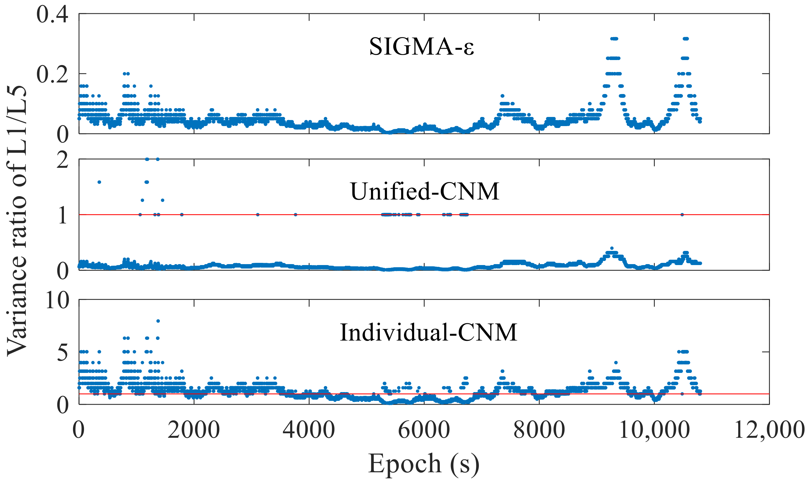
Table 3 lists the real-time differential root-mean-square (RMS) errors of different stochastic models using GPS L1/L5 + Galileo E1/E5a observations for the parameters of the unified-CNM and individual-CNM models described in Section 3.1.1. The RMS values along the three directions for the individual-CNM model are the smallest, followed by those for the elevation model. However, the results of the SIGMA-ε and unified-CNM models are all worse than those of the elevation model in the real-time differential analysis. Thus, the proposed individual-CNM model provides optimal results.

Table 3. Real-time differential root-mean-square (RMS) errors of different stochastic models for three directions.

Stochastic Model	East (m)	North (m)	Up (m)
Elevation	2.26	2.08	5.29
SIGMA-ε	2.36	2.25	5.50
Unified-CNM	2.48	2.53	5.99
Individual-CNM	2.00	2.00	4.93

Next, we used RTK positioning to evaluate the stochastic models. Table 4 lists the RTK positioning solutions of different stochastic models using GPS L1/L5 + Galileo E1/E5a observations. The positioning accuracy of every C/N0 model is better than that of the elevation model. However, in the C/N0 model, the SIGMA-ε and unified-CNM models take longer to converge. On the other hand, the accuracy of the individual-CNM model is the highest, and its convergence time is similar to that of the elevation model. Therefore, the individual-CNM model achieves the highest positioning performance.

Table 4. Real-time differential RMS errors of different stochastic models for positioning.

Stochastic Model	Convergence Time (min)	RMS Error after Convergence
		East (m)	North (m)	Up (m)
Elevation	44.1	0.067	0.029	0.064
SIGMA-ε	103.9	0.057	0.037	0.057
Unified-CNM	76.0	0.040	0.036	0.064
Individual-CNM	44.7	0.046	0.031	0.067

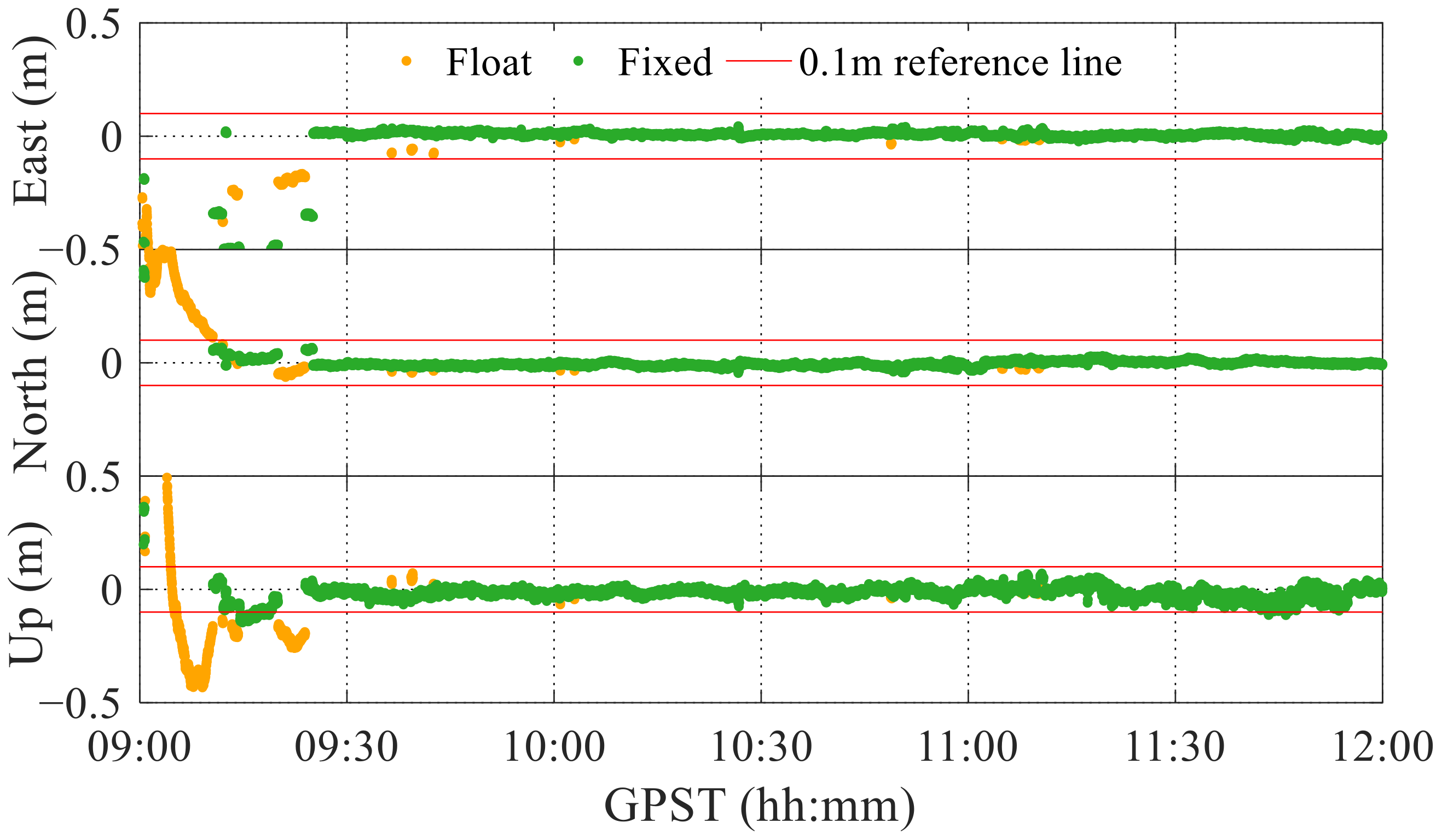
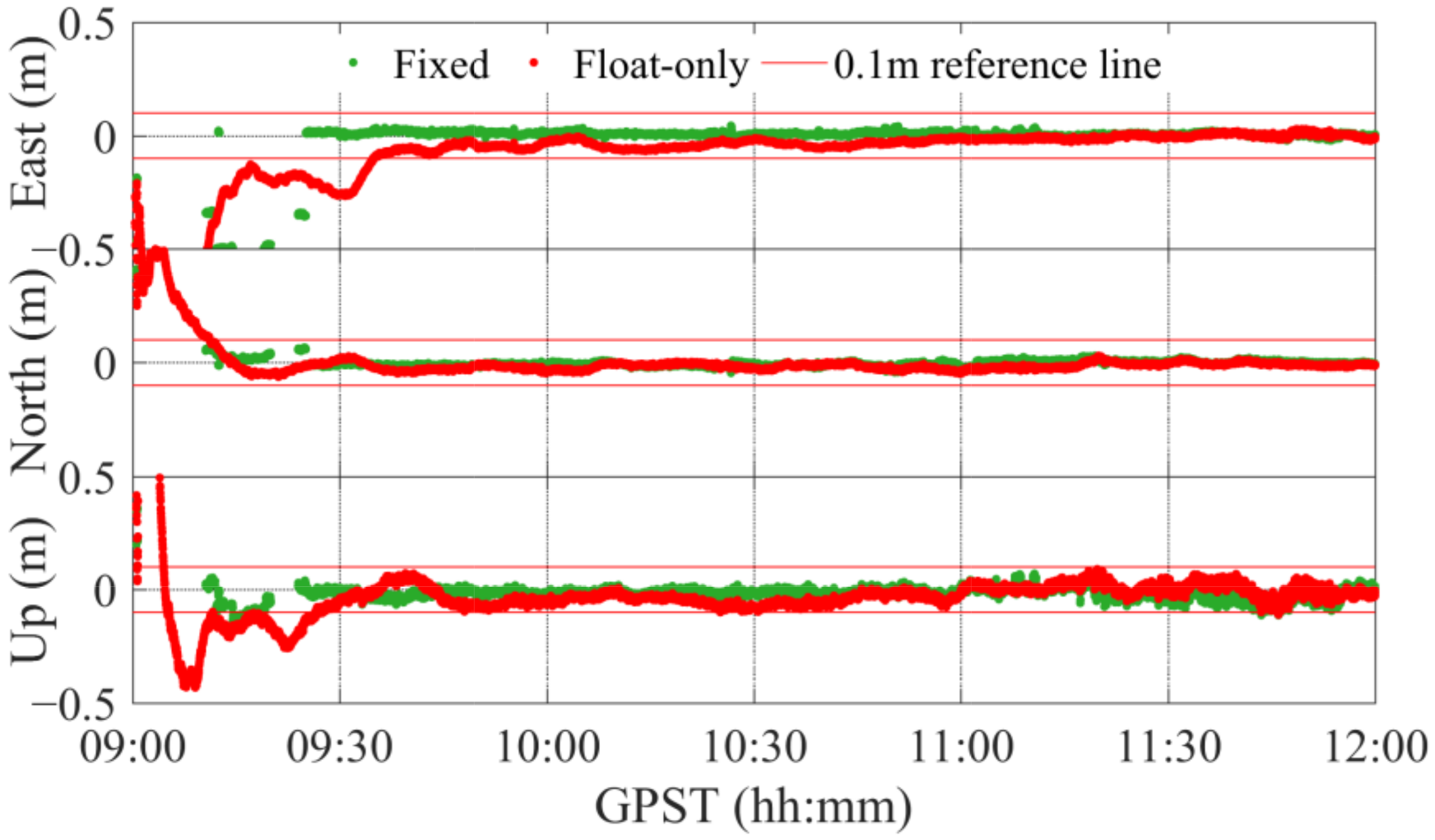
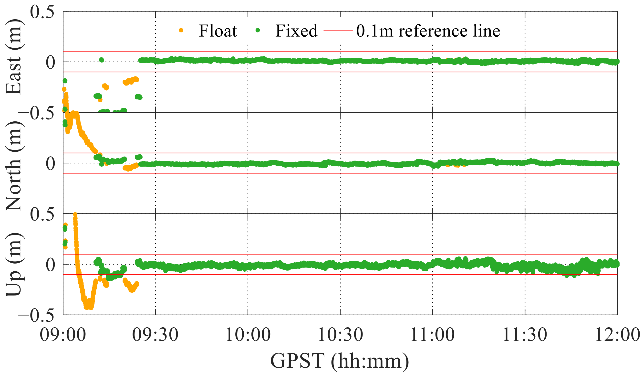
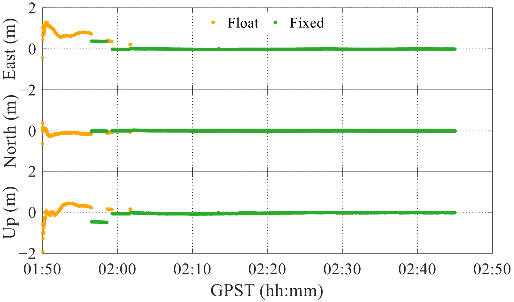
For ambiguity resolution, Figure 7 and Figure 8 show the fully fixed ambiguity and partially fixed ambiguity solutions for GPS L1 + Galileo E1 observations, respectively. Considering the results after 1500 s (around 9:30), most unfixed ambiguities can be fixed when using the partial resolution, effectively improving RTK positioning. A comparison of the fixed and float-only solutions is shown in Figure 9. Ambiguity resolution can substantially improve the positioning accuracy.

Figure 7. Results of full ambiguity resolution for GPS L1 + Galileo E1 observations.

Figure 8. Results of partial ambiguity resolution for GPS L1 + Galileo E1 observations.

Figure 9. Fixed and float-only solutions for GPS L1 + Galileo E1 observations.

Table 5 lists the statistical results of the float-only, full, and partial resolution. Overall, the accuracy of fixed solutions is higher than that of float-only solutions, and partial resolution can considerably improve the fixing rate, positioning accuracy, and convergence speed. However, there are also some error-fixed solutions.

Table 5. Statistical results for GPS L1 + Galileo E1 observations.

Fixed Mode	Fixing Rate (%)	Error-Fixing Rate (%)	Convergence Time (min)	RMS Error after Convergence
				East (m)	North (m)	Up (m)
Float ambiguity	–	–	35.0	0.035	0.020	0.043
Full resolution	63.4	0	35.0	0.018	0.014	0.031
Partial resolution	90.4	5.3	25.1	0.012	0.012	0.026

In the parameter settings, five epochs (i.e., minimum lock) should converge before participating in ambiguity resolution when a cycle slip occurs, aiming to mitigate the influence of cycle slips. To further weaken the influence of cycle sips, the fix-and-hold mode [29] is used to impose a tight constraint on fixed ambiguities. This mode uses the fixed ambiguity solutions as virtual observations and performs secondary filtering to improve the filtering covariance matrix, aiming to reduce the influence of state initialisation on the covariance.

Only when the ratio reaches 10.0 or higher do we use the fix-and-hold mode for ambiguity resolution to ensure the reliability of fixed solutions. The corresponding solutions are shown in Figure 10. Compared with Figure 8, the positioning results are smoother after using the fix-and-hold mode. The fixing rate increases to 90.8% and up to 100% after convergence. Therefore, when the fixing rate is not low in the continuous mode, we also apply the fix-and-hold mode to improve the fixing rate.

Figure 10. Fixed ambiguity solutions using fix-and-hold mode for GPS L1 + Galileo E1 observations.

3.3. Evaluation of Ambiguity Resolution for Different Observation Combinations

Next, we evaluated the actual fixing rate and fixed-solution accuracy of different observation combinations to improve observation selection. The positioning parameters are as listed in Table 2. The solutions for single-frequency observations are listed in Table 6.

Table 6. Solutions for single-frequency observation combinations (G, GPS; R, GLONASS; E, Galileo; C, BDS).

Observation Combination	Mean Number of Satellites	Fixing Rate (%)	Error-Fixing Rate (%)	Convergence Time (min)	RMS Error after Convergence
					East (m)	North (m)	Up (m)
G	6.6	28.3	28.3	Non-convergent	–	–	–
C	6.5	3.3	3.2	Non-convergent	–	–	–
G/C	13.1	55.6	5.9	71.7	0.011	0.015	0.021
G/E	10.0	90.8	5.3	25.1	0.012	0.011	0.025
G/E/C	16.5	60.7	12.4	58.3	0.012	0.009	0.019
G/R/E/C	21.2	49.7	0.8	36.3	0.023	0.009	0.022
G/C (no GEO)	11.2	80.3	0	23.0	0.013	0.016	0.026
G/E/C (no GEO)	14.6	85.7	0	32.5	0.013	0.012	0.017
G/E/C (no GEO/float C)	14.6	88.5	2.9	25.0	0.012	0.010	0.022

No GEO, exclude BDS GEO satellites; float C, BDS satellites do not participate in ambiguity resolution; non-convergent, positioning accuracy remained above 0.1 m.

Table 6 shows that when using single-constellation and single-frequency observations, the mean number of satellites is approximately six, and thus the fixing rates are low and cannot converge. When using the G/C combination, which nearly doubles the number of satellites, the fixing rate increases to 55.6%, but it remains low and has a slow convergence. On the other hand, the fixing rate of the G/E combination can reach 90.8% and converges after 25.1 min, indicating substantial improvement in both the fixing rate and convergence time.

When using combinations G/E/C and G/R/E/C, the number of satellites greatly increases, but the fixing rate decreases drastically, possibly due to anomalies in the BDS and GLONASS observations acquired by the smartphone. After analysis, we found that for combination G/C or G/E/C, after excluding the BDS GEO and GLONASS satellite observations, the fixing rate increases to 80.3% and 85.7%, respectively, and the convergence speed also increases. This is mainly attributable to the GEO satellite observations in smartphones, which have a half-cycle jump, and the GEO satellite itself has a very poor orbit accuracy [30]. Figure 11 shows that in the observations from the two BDS GEO satellites, C01 and C03, the carrier-phase residuals of the float solutions in many epochs are close to 0.5, likely corresponding to half-cycle jumps. However, the half-cycle jumps are very difficult to detect. Such jumps should be identified by the loss-of-lock indicator in the RINEX file or in field AccumulatedDeltaRangeState [4] of the GNSS raw measurements. In addition, in the combination of G/E/C, when excluding the BDS GEO satellite observations and not fixing the BDS ambiguities, the fixing rate increases again to 88.5%. The main reason is that the cycle slips of BDS are more frequent than those of other constellations (Figure 5). As frequent cycle slips severely undermine positioning, it is better not to fix the BDS ambiguity. In contrast, although GLONASS observations have fewer cycle slips, the fixing rate of combination G/R/E/C is also lower than that of combination G/E/C, mainly because the noise of GLONASS observations in smartphones is higher than that of observations from other constellations [6]. Therefore, for a suitable number of satellites, the cycle-slip satellites should be controlled to participate in positioning, and observations from the BDS GEO and GLONASS satellites should be avoided.

Figure 11. Half-cycle jump of BDS GEO satellite observations acquired by smartphone.

Further analysis of the combinations that include dual-frequency observations and other satellites with single-frequency data was also performed. The corresponding solutions are listed in Table 7. The fixing rate of the GPS dual-frequency observations is only 22.4%, which is lower than the single-frequency result, and the fixing rate of G/E single-frequency observations is relatively high, but the dual-frequency fixing rate is only 10.6%, being lower than that of the single-GPS constellation. The positioning accuracy also fails to converge within 0.1 m. If band L5 or E5a is not fixed, the fixing rate increases to 59.1% and 88.0%, respectively, mainly because the cycle slips in bands GPS L5 and Galileo E5a are extremely frequent, with those of band Galileo E5a being more frequent. The cycle-slip ratios in bands GPS L5 and Galileo E5a are 5.2% and 8.2%, respectively. When a cycle slip occurs in RTK positioning, the ambiguity parameters should be reinitialised, and frequent initialisation reduces the ambiguity fixing rate.

Table 7. Solutions of dual-frequency combinations. The mean number of satellites only includes dual-frequency satellites.

Observation Combination	Mean Number of Satellites	Fixing Rate (%)	Error-Fixing Rate (%)	Convergence Time (min)	RMS Error after Convergence
					East (m)	North (m)	Up (m)
G L1/L5	2.9	22.4	5.4	Non-convergent	–	–	–
G L1/L5 (float L5)		59.1	20.4	Non-convergent	–	–	–
G L1/L5 + E E1/E5a	5.8	10.6	8.7	Non-convergent	–	–	–
G L1/L5 + E E1/E5a (float L5/E5a)		88.0	3.6	30.8	0.013	0.011	0.024

In Table 7, the number of satellites with simultaneous dual-frequency observations is low, and their cycle slips are frequent, further reducing the availability of dual-frequency observations. Therefore, these observations are limited for use in long-baseline RTK positioning or precise point positioning and other multi-frequency combination positioning strategies.

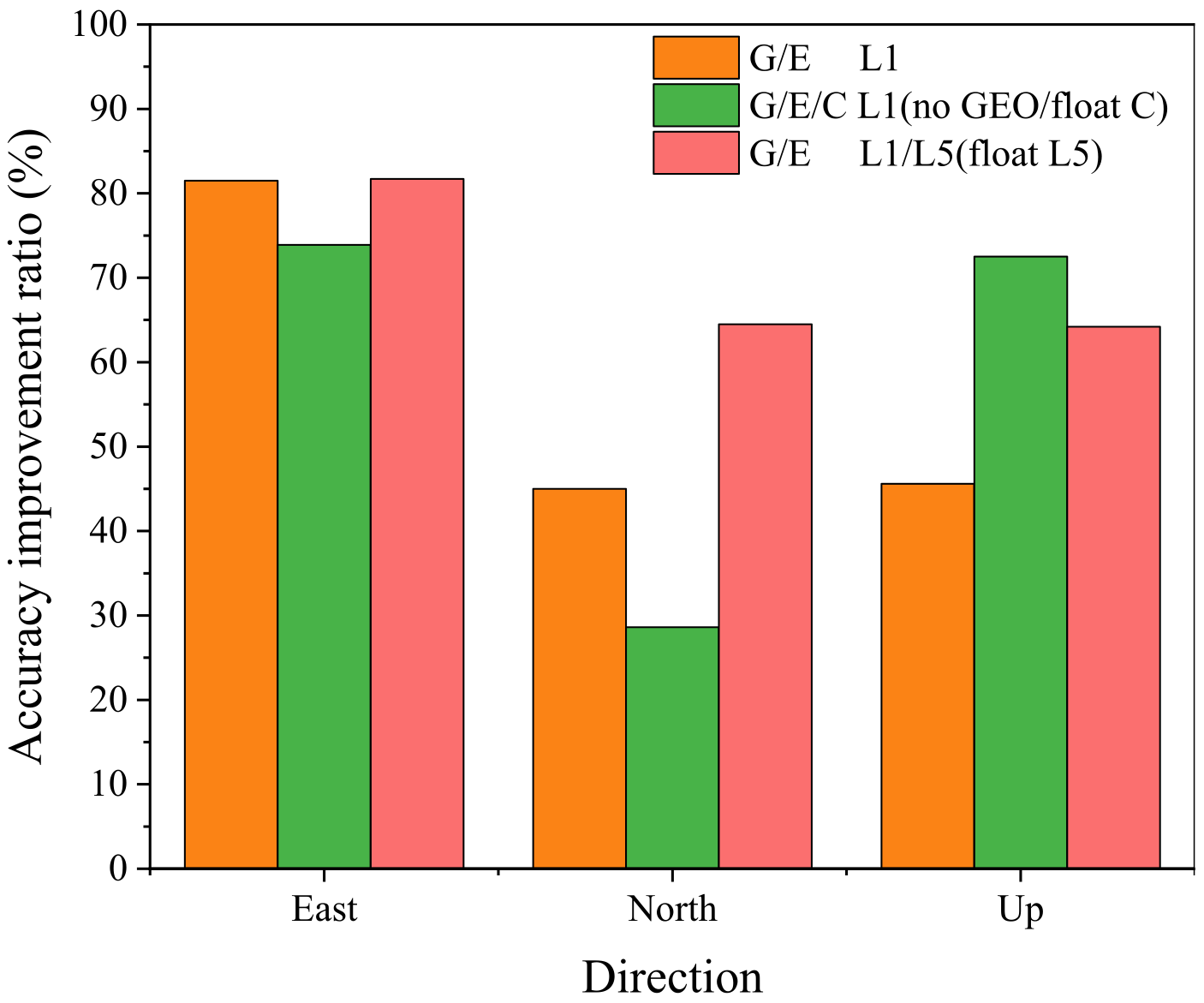
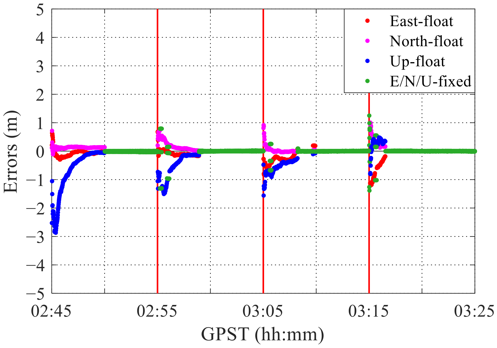
In the results reported above, the accuracy of fixed solutions using different observation combinations is consistent, and an accuracy of approximately 1 and 2 cm can be achieved along the horizontal and vertical directions, respectively. However, owing to the excessive noise in smartphone observations, even for a fixing rate above 90%, it is still difficult to obtain millimetre-level accuracy. For several combinations with a fixing rate higher than 88%, we compared the accuracy of the fixed solutions and their corresponding float solutions simultaneously after the fixed solutions converged, obtaining the results shown in Figure 12. After fixing the ambiguity, the accuracy along the three directions improves. The east direction shows the highest improvement, reaching approximately 80%, and the other two directions show improvements by more than 30%. Hence, ambiguity resolution is important for high-precision positioning in smartphones, and future work should pursue further improvements in the fixing rate while shortening the convergence time.

Figure 12. Accuracy of fixed solutions compared with corresponding float solutions.

The above analysis shows that the large difference in fixed rates for the different combinations is mainly due to the impact of the number of satellites, cycle slips, and observation accuracy. By considering the results above, the correct fixing rate, and a reasonable convergence time, we recommend using combination G/E/C (no GEO/float C) for poisoning based on smartphone observations when the number of satellites is sufficient.

3.4. Analysis of RTK-Positioning Convergence Time by Segment

To verify the consistency of the convergence time in different periods, we solved the entire observation data in segments, that is, we reinitialised the coordinates and ambiguity parameters in a segments once every 1 h, and then solved the segments separately. As reported above, the combination G/E/C of single-frequency observations provides the best convergence overall. Thus, we used it for data processing without resolving the BDS ambiguity. The other calculation parameters were set as listed in Table 2. Considering slow convergence, we started to fix the ambiguity after 3 min of observations.

In addition to the data from 15 November 2020, which were used above, we used two additional datasets collected in recent days, at the same location and with a similar setup. The data collected on 11 November 2020 are approximately of 3 h, and the data collected on 14 November 2020 are approximately of 5 h. Here, we used the last 3 h of the 5 h data for analysis, owing to the clock jump in the previous data, and it will not affect the results of the segmented solution. These two datasets mainly aim to increase the amount of data for convergence time analysis and do not consider the impact of geomagnetic storm conditions on different days.

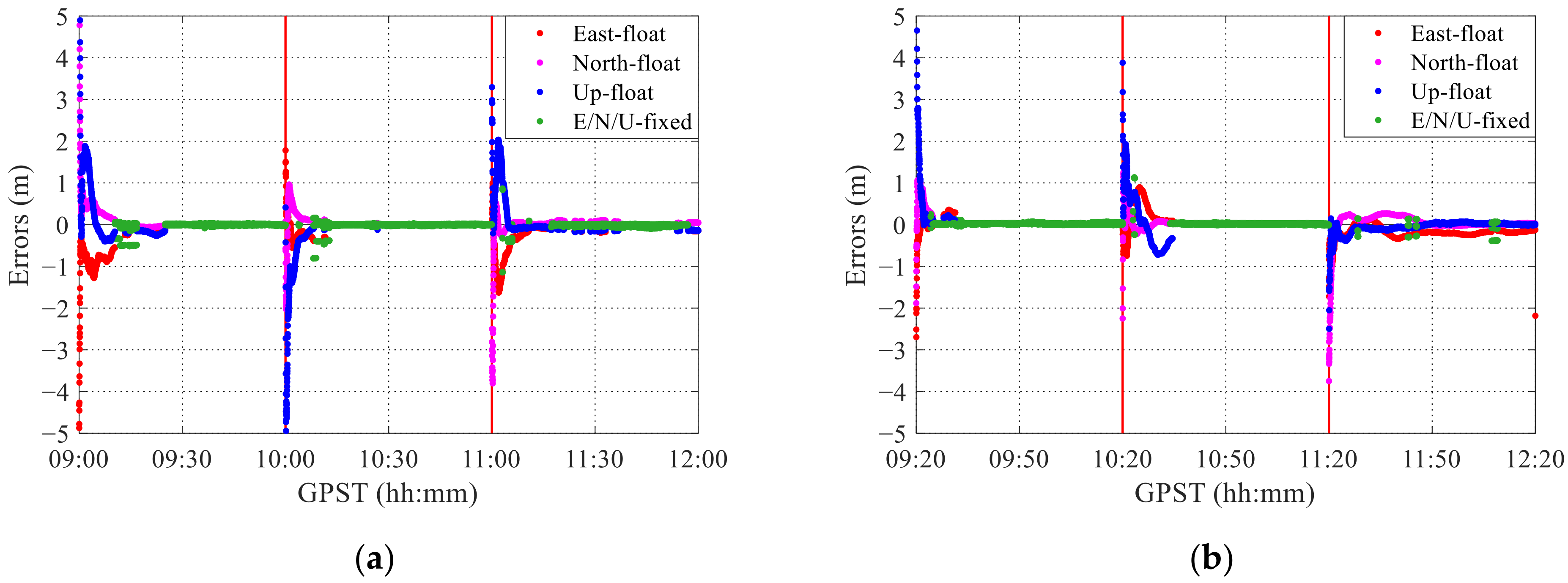
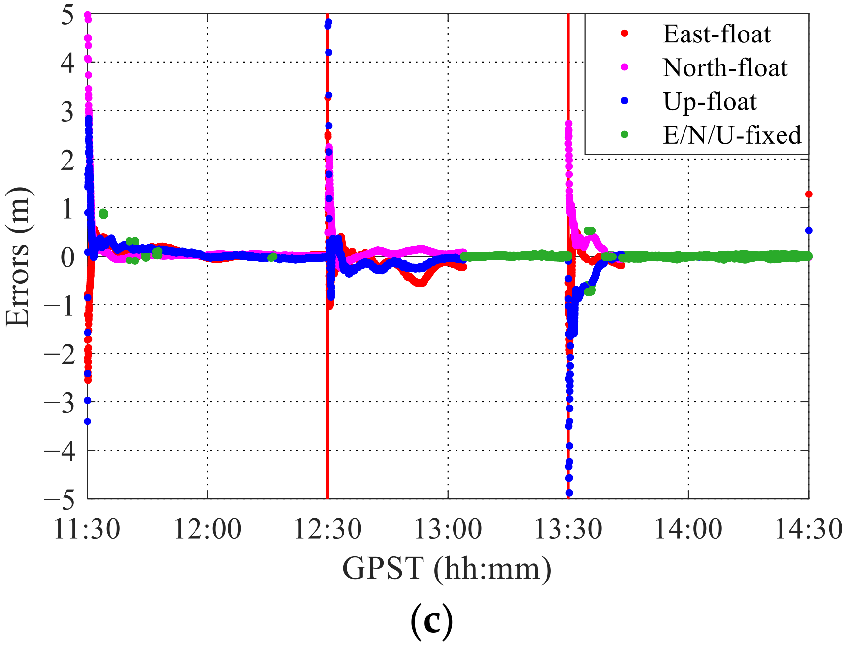
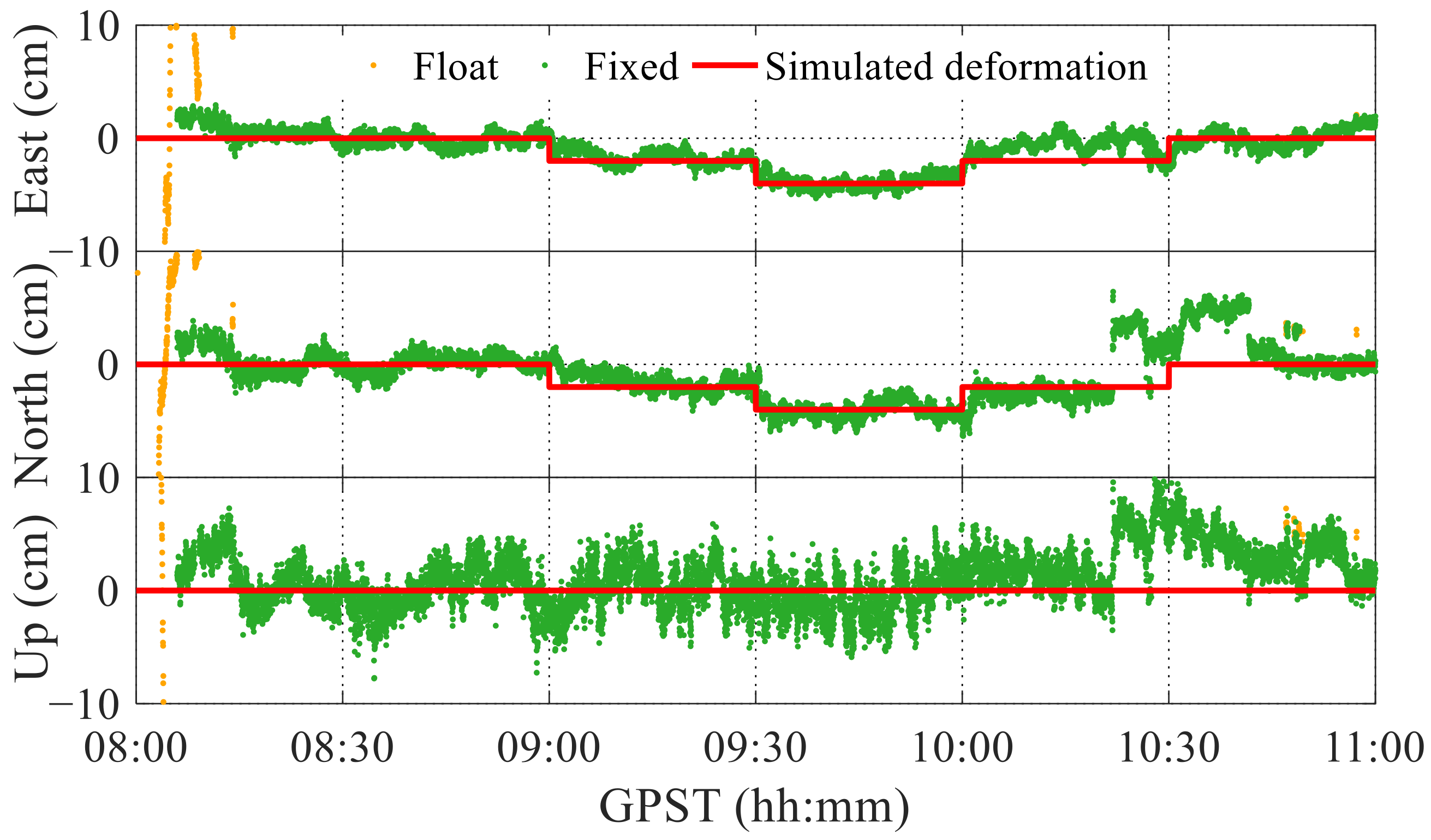
Figure 13 shows the segmented solutions for 1 h intervals. Table 8 lists the convergence time of each session, the mean number of satellites in combination G/E (as BDS is not fixed, the number of BDS satellites is not considered), and the mean number of candidate ambiguities that meet the fixed conditions (e.g., C/N0 threshold, cycle slip). The convergence time differs across segments, mostly being 10–20 min and exceeding 30 min for few segments. In addition, the ambiguity can hardly be resolved for two segments mainly because the number of candidate ambiguities is very small. The corresponding segment with a long convergence time usually has few candidate ambiguities. For example, for segment 1 of dataset 2, the number of candidates is the largest, achieving the fastest convergence, whereas for segment 3 of dataset 2 and segment 1 of dataset 3, the number of candidates is lower than 1 (0.4 and 0.2, respectively), and the ambiguity cannot be fixed. Even if the total number of satellites is large, when a satellite elevation and C/N0 are very low or a cycle slip occurs, the corresponding ambiguity does not meet the fixed conditions and cannot be used for ambiguity resolution, resulting in few candidate ambiguities. On the other hand, the results in Section 3.3 show that simply including the number of observations from other constellations or frequencies in ambiguity resolution is not conducive to a higher fixing rate.

Figure 13. Results of segmented solutions over 1 h intervals for data acquired over 3 days. (a) Dataset 1 collected on 15 November 2020, (b) dataset 2 collected on 11 November 2020, and (c) dataset 3 collected on 14 November 2020.

Table 8. Statistical results of solutions per segment.

Dataset	Segment	Convergence Time (min)	Mean Number of G/E Satellites	Mean Number of Candidate Ambiguities	Cycle-Slip Rate (%)	Pseudo-Range RMS Residual (m)
1	1	25.0	10.4	5.4	1.03	5.05
	2	12.8	10.9	7.7	0.12	4.37
	3	17.3	8.7	3.7	0.35	5.07
2	1	13.0	11.2	8.0	0.37	5.87
	2	14.5	11.4	7.2	0.07	5.04
	3	Not fixed	11.1	0.4	0.35	5.28
3	1	Not fixed	8.5	0.2	1.34	4.74
	2	33.9	8.2	4.0	0.17	4.66
	3	13.3	9.3	7.2	0.31	4.60

Table 8 shows that the cycle-slip rate may not determine the number of candidates directly because it is also related to other factors, but a large number of candidates must correspond to a low cycle-slip rate. The pseudo-range residuals are approximately 5 m, and there is no obvious correlation with the fixing rate. However, the pseudo-range accuracy is the main factor influencing the main convergence speed [31], but it can be superseded by other factors such as the cycle slips. The effect of the cycle-slip rate and pseudo-range accuracy on convergence is reported in Section 5. Nevertheless, we can conclude that higher-quality GPS and Galileo observations increase the number of candidate ambiguities, accelerate convergence, and increase the fixing rate.

4. Evaluation of Dynamic Deformation Monitoring Using Smartphone

The results reported above show that the RTK positioning accuracy of a smartphone can reach 1 cm, suggesting its potential for surveying and mapping applications. Hou et al. [32] studied the feasibility of a low-cost u-blox receiver for dynamic deformation monitoring in high-rise buildings, and Uradziński et al. [17] evaluated the static solution accuracy of smartphones in geodetic applications. Similarly, we explored the feasibility of using mass-produced smartphones as deformation monitoring devices through an experiment using simulated deformation equipment.

As shown in Figure 14, the simulated deformation equipment can move along the east, north, and up directions and register the displacement. Before conducting the experiment, we calibrated the true north using a compass. A Xiaomi Mi 8 smartphone was then fixed on the simulation platform and its body was kept upright to ensure adequate signal reception.

Figure 14. Experimental setup for simulated dynamic deformation monitoring.

During the experiment, the equipment was displaced once every 30 min to simulate the dynamic deformation of the monitored body. Considering the low accuracy of smartphone GNSS dynamic positioning, the horizontal displacement was set to 2 cm per movement. The schedule of the simulated deformation is listed in Table 9.

Table 9. Schedule of simulated deformation.

Moving Time (GPST)	North Displacement (mm)	East Displacement (mm)
08:00 (start)	0	0
08:30	0	0
09:00	−20	−20
09:30	−20	−20
10:00	20	20
10:30	20	20
11:00 (end)	0	0

For this experiment, we used GPS L1 observations to obtain the solutions, as there were few Galileo and BDS satellites in common view with the base station during the measurements. In addition, the ambiguity resolution mode was fix-and-hold. In the experiment, the average fixed solutions before the smartphone displaced in 1 h were used as the initial reference coordinates. The experimental results are shown in Figure 15. Centimetre-level accuracy is achieved as well as a fixing rate of 96.2%. In 9:00–9:30 and 9:30–10:00, the solutions suitably agree with the simulated deformation, and the deformation can be clearly seen at 9:00, 9:30, and 10:00. In the second half of the period 10:00–10:30 and the first half of the period 10:30–11:00, the solutions shift due to cycle slips, but they return to normal after some periods.

Figure 15. Results of simulated dynamic deformation monitoring using smartphone.

The experimental results show that the deformation trend can be determined by using a smartphone, but owing to its high observation noise, deformation monitoring at the millimetre level cannot be achieved. In addition, a smartphone is extremely susceptible to interference from the environment and its own components during measurement. Consequently, it may not be applicable to actual monitoring scenarios at this stage of development. Improving the GNSS hardware quality in smartphones may enable monitoring applications in mass-produced smartphones.

5. Discussion

In this study, we mainly evaluated the RTK positioning accuracy and ambiguity resolution using the built-in antenna of a smartphone for GNSS observations. The results show that cycle slips are very frequent in smartphones, considerably undermining high-precision positioning. In addition to accurate cycle-slip detection, the frequency of cycle slips in smartphones should be mitigated. Although adopting appropriate strategies can increase the fixing rate, it remains low, and correct fixation takes a long time initially. Moreover, the highest accuracy can reach 1 cm, even if the ambiguity is fixed correctly. Observation noise and changes in the antenna phase centre may hinder additional improvements in the positioning performance through data processing.

The low fixing rate and low positioning accuracy can be explained by the use of low-cost antennas that have low gain and low multipath resistance, resulting in low-accuracy pseudo-range and carrier-phase observations. Improving the antenna design is essential to improve the fixing-rate reliability and reduce the convergence time. To illustrate this concept, we used a choke coil for the geodetic antenna in auxiliary experiments. The smartphone was placed upright on the choke coil to reduce the effect of multipath signals, as shown in Figure 16. Approximately 1.5 h of data were collected from 1:50 to 3:25 (GPS Time). Since the data were sufficiently long, we partitioned the data into two subsets. Similar to the previous analysis, the first subset (before 2:45) was utilized to examine the long-term stability of fixed solutions, while the second subset (after 2:45) was used for convergence time analysis in tiny segments. The observation selection and calculation parameter settings were the same as those in Section 3.4.

Figure 16. Experiments using choke coil to suppress multipath interference.

The results of long-term RTK positioning using the choke coil are shown in Figure 17, with a 92.4% fixing rate. It can be observed that the error is less than 2 m in the initial stage, which is better than when the choke coil is not used. Moreover, the solution can remain fixed for about 10 min after the start, and the error remains stable.

Figure 17. Results of long-term RTK positioning in choke-coil experiment.

Following that, we analyzed the segmented RTK positioning in detail. Because the ambiguity can be resolved within 10 min in the initial stage, the calculation segment interval was likewise set to 10 min. The results are shown in Figure 18 and Table 10. It can be seen that the time to fix ambiguity was shortened to less than 5 min, with the fastest fixation taking only 1.5 min. Even though it took nearly 10 min to be fixed in the initial stage, it was much shorter than the time when using the built-in smartphone antenna. In addition, the positioning accuracy after convergence was higher than when the choke coil was not used. In segment 4, the RMS errors along the east, north, and up directions were 0.003, 0.004, and 0.007 m, respectively, showing millimetre-level accuracy. After using the choke coil, the mean number of candidate ambiguities was relatively large, and there were almost no cycle slips. In addition, the pseudo-range accuracy was approximately 2 m, representing an increase of more than 50%.

Figure 18. Results of RTK segmented positioning in choke-coil experiment.

Table 10. Statistical results of RTK segmented positioning in choke-coil experiment.

Segment	Convergence Time (min)	RMS Error of Fixed Solution			Mean Number of Candidate Ambiguities	Cycle-Slip Rate (%)	Pseudo-Range RMS Residual (m)
		East (m)	North (m)	Up (m)
1	5.0	0.021	0.004	0.023	6.0	0.0	2.15
2	3.9	0.008	0.004	0.011	7.6	0.0	2.10
3	3.2	0.004	0.004	0.012	7.4	0.0	2.26
4	1.5	0.003	0.004	0.007	8.9	0.0	2.12

The choke coil experiment confirms that the antenna design is essential to improve the fixing rate, convergence speed, and positioning accuracy because it increases the observation quality. Although external antennas and choke coils are also used to improve the positioning performance of smartphones, they may not be the best choice for practical applications. We expect that manufacturers will continuously improve the quality of GNSS modules in smartphones, while we continue to study optimisation algorithms for positioning. In future research, we can make full use of the advantages of smartphones equipped with multiple sensors, in order to make up for the shortcomings of a single GNSS through integration of GNSS/IMU and other sensors. As they do not cause changes in coordinates during deformation monitoring that are too large, coordinate or baseline constraints may be used to improve the positioning effect.

6. Conclusions

We comparatively analysed the quality of multi-frequency GNSS observations in the Xiaomi Mi 8 smartphone. The analysis results allowed us to use improved algorithms including a stochastic model and ambiguity resolution for short-baseline RTK positioning. The ambiguity fixing rate, positioning performance, and convergence time using only the embedded smartphone GNSS antenna were then determined. The feasibility of using a smartphone for dynamic deformation monitoring was also verified. The cycle slips in the smartphone were severe, especially when C/N0 was below 30 dB-Hz. In addition, C/N0 of band L5/E5a was lower than that of band L1/E1, and its cycle-slip ratio was higher than that of band L1/E1, limiting the use of the second frequency in smartphones. In future work, we will explore the effective use of the second frequency for GNSS observations.

Using an improved C/N0 stochastic model and partial ambiguity resolution combined with other solving strategies can improve the positioning accuracy and ambiguity fixing rate. The ambiguity fixing rate varies greatly with different combinations of observations, and it is mainly affected by the number of satellites and cycle slips. It can reach 80–90% or above. The solution using GPS + Galileo + BDS single-frequency combination while keeping the BDS float ambiguity is the best, and its ambiguity fixing rate can reach approximately 90% in 3 h observations. However, it still takes a long time (usually 10–30 min) for a fixed solution to converge within 0.1 m. The accuracy of the fixed solutions for different band combinations can reach 1 and 2 cm along the horizontal and vertical directions, respectively.

By simulating dynamic deformation monitoring, the smartphone can recognise 2 cm deformation trends, being insufficient for actual monitoring applications. Nevertheless, a smartphone may be applied for high-precision measurements in applications such as vibration monitoring.

After using a choke coil around the smartphone, the fixing rate, convergence speed, and positioning accuracy improve, demonstrating the importance of antenna design on the positioning performance. With the advancement of hardware development, improved GNSS modules may lead to fast centimetre- or millimetre-level positioning accuracy in smartphones.

References

- The European GNSS Agency. GNSS Market Report 2017; The European GNSS Agency: Prague, Czech Republic, 2017. [Google Scholar]
- Paziewski, J. Recent advances and perspectives for positioning and applications with smartphone GNSS observations. Meas. Sci. Technol 2020, 31, 091001. [Google Scholar] [CrossRef]
- Aggrey, J.; Bisnath, S.; Naciri, N.; Shinghal, G.; Yang, S. Multi-GNSS precise point positioning with next-generation smartphone measurements. J. Spatial Sci. 2019, 65, 79–98. [Google Scholar] [CrossRef]
- White Paper on Using GNSS Raw Measurements on Android Devices; European GNSS Agency: Prague, Czech Republic, 2017.
- Zhang, X.; Tao, X.; Zhu, F.; Shi, X.; Wang, F. Quality assessment of GNSS observations from an Android N smartphone and positioning performance analysis using time-differenced filtering approach. GPS Solut. 2018, 22, 70. [Google Scholar] [CrossRef]
- Liu, W.; Shi, X.; Zhu, F.; Tao, X.; Wang, F. Quality analysis of multi-GNSS raw observations and a velocity-aided positioning approach based on smartphones. Adv. Space Res. 2019, 63, 2358–2377. [Google Scholar] [CrossRef]
- Li, G.; Geng, J. Characteristics of raw multi-GNSS measurement error from Google Android smart devices. GPS Solut. 2019, 23, 90. [Google Scholar] [CrossRef]
- Robustelli, U.; Baiocchi, V.; Pugliano, G. Assessment of dual frequency GNSS observations from a Xiaomi Mi 8 Android smartphone and positioning performance analysis. Electronics 2019, 8, 91. [Google Scholar] [CrossRef] [Green Version]
- Realini, E.; Caldera, S.; Pertusini, L.; Sampietro, D. Precise GNSS positioning using smart devices. Sensors 2017, 17, 2434. [Google Scholar] [CrossRef] [Green Version]
- Dabove, P.; Di Pietra, V. Single-baseline RTK positioning using dual-frequency GNSS receivers inside smartphones. Sensors 2019, 19, 4302. [Google Scholar] [CrossRef] [Green Version]
- Dabove, P.; Di Pietra, V. Towards high accuracy GNSS real-time positioning with smartphones. Adv. Space Res. 2019, 63, 94–102. [Google Scholar] [CrossRef]
- Liu, J.; Deng, C.; Tang, W. Review of GNSS ambiguity validation theory. Geomat. Inf. Sci. Wuhan Univ. 2014, 39, 1009–1016. [Google Scholar]
- Wanninger, L.; Heßelbarth, A. GNSS code and carrier phase observations of a Huawei P30 smartphone: Quality assessment and centimeter-accurate positioning. GPS Solut. 2020, 24, 1–9. [Google Scholar] [CrossRef] [Green Version]
- Geng, J.; Li, G. On the feasibility of resolving Android GNSS carrier phase ambiguities. J. Geod. 2019, 93, 2621–2635. [Google Scholar] [CrossRef]
- Bochkati, M.; Sharma, H.; Lichtenberger, C.A.; Pany, T. Demonstration of fused RTK (fixed) + inertial positioning using Android smartphone sensors only. In Proceedings of the 2020 IEEE/ION Position, Location and Navigation Symposium (PLANS), Portland, OR, USA, 20–23 April 2020; pp. 1140–1154. [Google Scholar]
- Gao, R.; Xu, L.; Zhang, B.; Liu, T. Raw GNSS observations from Android smartphones: Characteristics and short-baseline RTK positioning performance. Meas. Sci. Technol. 2021, 32, 084012. [Google Scholar] [CrossRef]
- Uradziński, M.; Bakuła, M. Assessment of static positioning accuracy using low-cost smartphone GPS devices for geodetic survey points’ determination and monitoring. Appl. Sci. 2020, 10, 5308. [Google Scholar] [CrossRef]
- Tomaštík, J.; Chudá, J.; Tunák, D.; Chudy, F.; Kardoš, M. Advances in smartphone positioning in forests: Dual-frequency receivers and raw GNSS data. For. Int. For. Res. 2020, 94, 292–310. [Google Scholar] [CrossRef]
- Lu, L.; Ma, L.; Liu, W.; Wu, T.; Chen, B. A triple checked partial ambiguity resolution for GPS/BDS RTK positioning. Sensors 2019, 19, 5034. [Google Scholar] [CrossRef] [Green Version]
- Logging of GNSS Raw Data on Android. Available online: http://www.geopp.de/logging-of-gnss-rawdata-on-android/ (accessed on 10 January 2020).
- Netthonglang, C.; Thongtan, T.; Satirapod, C. GNSS Precise Positioning determinations using smartphones. In Proceedings of the 2019 IEEE Asia Pacific Conference on Circuits and Systems (APCCAS), Bangkok, Thailand, 11–14 November 2019; pp. 401–404. [Google Scholar]
- Guo, L.; Wang, F.; Sang, J.; Lin, X.; Gong, X.; Zhang, W. Characteristics analysis of raw multi-GNSS measurement from Xiaomi Mi 8 and positioning performance improvement with L5/E5 frequency in an urban environment. Remote Sens. 2020, 12, 744. [Google Scholar] [CrossRef] [Green Version]
- Zhao, S.; Cui, X.; Guan, F.; Lu, M. A Kalman Filter-Based Short Baseline RTK Algorithm for Single-Frequency Combination of GPS and BDS. Sensors 2014, 14, 15415–15433. [Google Scholar] [CrossRef]
- Hartinger, H.; Brunner, F.K. Variances of GPS phase observations: The SIGMA-ɛ model. GPS Solut. 1999, 2, 35–43. [Google Scholar] [CrossRef]
- Wang, L.; Li, Z.; Wang, N.; Wang, Z. Real-time GNSS precise point positioning for low-cost smart devices. GPS Solut. 2021, 25, 69. [Google Scholar] [CrossRef]
- Wen, Q.; Geng, J.; Li, G.; Guo, J. Precise point positioning with ambiguity resolution using an external survey-grade antenna enhanced dual-frequency android GNSS data. Measurement 2020, 157, 107634. [Google Scholar] [CrossRef]
- Teunissen, P.J.G. The least-squares ambiguity decorrelation adjustment: A method for fast GPS integer ambiguity estimation. J. Geod. 1995, 70, 65–82. [Google Scholar] [CrossRef]
- Takasu, T.; Yasuda, A. Development of the low-cost RTK-GPS receiver with an open source program package RTKLIB. In Proceedings of the International symposium on GPS/GNSS, International Convention Center, Jeju, Korea, 21–24 October 2014; pp. 4–6. [Google Scholar]
- Takasu, T.; Yasuda, A. Kalman-filter-based integer ambiguity resolution strategy for long-baseline RTK with ionosphere and troposphere estimation. In Proceedings of the 23rd International Technical Meeting of the Satellite Division of the Institute-of-Navigation (ION GNSS-2010), Portland, OR, USA, 21–24 September 2010; pp. 161–171. [Google Scholar]
- Liu, Y.; Ye, S.; Song, W.; Li, Q. Estimating the orbit error of BeiDou GEO satellites to improve the performance of multi-GNSS PPP ambiguity resolution. GPS Solut. 2018, 22, 1–14. [Google Scholar] [CrossRef]
- Mohammed, A.G.; Mosbeh, R.K.; Mostafa, M.R.; Zaki, M.Z. Improving Precise Point Positioning Convergence Time through TEQC Multipath Linear Combination. J. Surv. Eng. 2018, 144, 04018002. [Google Scholar]
- Hou, H.; Wang, Y.; Kuang, C. Feasibility analysis on dynamic deformation monitoring of high-rise buildings by low-cost GNSS receivers. J. Navig. Position 2019, 7, 94–98. [Google Scholar]
Publisher’s Note: MDPI stays neutral with regard to jurisdictional claims in published maps and institutional affiliations. |
© 2022 by the authors. Licensee MDPI, Basel, Switzerland. This article is an open access article distributed under the terms and conditions of the Creative Commons Attribution (CC BY) license (https://creativecommons.org/licenses/by/4.0/).