Fault Diagnosis via Neural Ordinary Differential Equations

Abstract

Implementation of model-based fault diagnosis systems can be a difficult task due to the complex dynamics of most systems, an appealing alternative to avoiding modeling is to use machine learning-based techniques for which the implementation is more affordable nowadays. However, the latter approach often requires extensive data processing. In this paper, a hybrid approach using recent developments in neural ordinary differential equations is proposed. This approach enables us to combine a natural deep learning technique with an estimated model of the system, making the training simpler and more efficient. For evaluation of this methodology, a nonlinear benchmark system is used by simulation of faults in actuators, sensors, and process. Simulation results show that the proposed methodology requires less processing for the training in comparison with conventional machine learning approaches since the data-set is directly taken from the measurements and inputs. Furthermore, since the model used in the essay is only a structural approximation of the plant; no advanced modeling is required. This approach can also alleviate some pitfalls of training data-series, such as complicated data augmentation methodologies and the necessity for big amounts of data.

1. Introduction

Fault diagnosis systems are of great importance in industrial processes, especially in those with high stakes systems, where it is important to perform continuous diagnostics and monitoring of the main variables. Furthermore, it could also be used to perform fault prediction for improving the maintenance plan and to avoid undesired malfunctions. In the fault detection literature, a great number of methods have been dedicated to model-based techniques [1,2] with great success in many cases, although a known drawback of such methods is their limitation to processes with relatively simple dynamics and sensiblity to model approximations. Examples of model-based methods are: the structural approach, which searches for irreducible relations that attains sensibility to the selected faults [3,4], and eigenstructure-based fault diagnosis, which deals with a minimization problem for the sensibility of perturbations against faults [5,6]. The same minimization problem is approached using Linear Matrix Inequalities (LMI) [7], and another common approach is to use observers, such as sliding mode observers [8], Kalman-based fault detection [9], and also residuals generation using parity space relations [10,11]. Likewise, for complex processes with functional constraints, methods have been developed that consider decentralized and distributed diagnostic architectures [12,13].

Another important group of fault detection techniques, regarded as data-based approaches, are used when the model of the plant under evaluation is not available. They are dedicated to the analysis of collected data to detect unusual trends in it, and thus identify faults in the system. Principal Component Analysis (PCA) performs a dimensionality reduction of the data map for finding faults in the system, although it requires high amounts of data [14,15]. Support Vector Machines (SVM) is a technique for classification that performs high generalization even with small data-sets but can suffer from data imbalance, although learning ability can be added such as in the multikernel SVM [16]. Artificial neural networks (ANN) are employed using supervised training and can detect faults after learning hidden relations in the data [17]; however, they lack visual representation and can suffer from overfitting. Use of Deep Learning (DL) techniques have become increasingly popular in the latter years due to an increase in power computation, higher availability of information, and high accuracy, many DL models have been tested such as Dense Neural Networks [18], Deep Belief Networks [19,20,21], Convolutional Neural Networks [22,23], Recurrent Neural Networks [24,25], and Generative Neural Networks [26], however, in most of the examples the DL model is adapted only to the plant in the study, therefore a change of plant will require a change of the methodology.

Some works have also been devoted to the elaboration of hybrid techniques, model-based plus data-based systems for fault diagnosis. These techniques aim to have combined advantages from both previously mentioned approaches, they use mainly machine learning techniques for fault identification coupled with model-based fault detectors. In [27], a hybrid model-based and data-driven system is elaborated for fault detection and diagnosis, although both methods are used independently. In [28], Jung proposed the use of SVM to improve fault identification, and in [29], the merging mechanism between residuals and SVM is improved for fault location. In [30], the hybrid mechanism is used for the selection of residual generators. Meanwhile, in [31], a Modified PCA was combined with filters to detect faults. On the other hand, the use of DL techniques in hybrid fault diagnosis systems has not been extensively developed, although the use of DL is recognized for improving accuracy in many other recognition tasks [32].

Deep neural networks are composed of finite transitions, in [33] the Neural Ordinary Differential Equations (Neural ODE) was presented using an idea inspired in ResNets [34] to give continuity to the network layers using ODE solvers, this development has been resembled and employed in many fields such as [35] for continuous graph flows that can be applied in generative tasks, moreover, it can be used to represent dynamics such as in [36] for Hamiltonian processes, in [37] for an extension of stochastic processes, and in [38] for inclusion in Graph Neural Networks as a tool to have a continuous flow of node features. These groundbreaking developments make the application of DL networks for hybrid fault detection systems very natural.

In this research, we embedded a preliminary plant model in the Neural ODE network; this network receives the measurements and inputs of the plant, given in state-space representation, and mirrors its corresponding dynamics. The training is performed in two phases; the Neural ODE is trained in the first stage in order to mimic the plant dynamics, and later it is conditioned to be used for the fault diagnosis system, which is trained in the second stage. The preliminary model is employed on behalf of two desired aspects: to have a more robust network behavior and reduce the training complexity. Since the Neural ODE allows us to represent the dynamics of a process, then the first aspect is demonstrated using an approximated (preliminary) plant model. We show that this is beneficial in comparison to model-less neural networks. Additionally, the Neural ODE’s internal dynamics permits us to have a visual representation of the network state.

The article is divided as follows, in Section 2 we present the theory for Neural ODE. Section 3 is dedicated to model representation and how Neural ODE is used for the implementation. In Section 4, a nonlinear benchmark model is used to illustrate the application of the approach. In Section 5, a visual representation of the network is proposed. In Section 6 the characteristics of the methodology are discussed. Finally in Section 7, some conclusions are given.

2. Graph Neural Ordinary Differential Equations

Resnet networks are shown to be one inspiration for the key concept of continuum layers in the neural ODE network. However, the neural ODE training poses the problem of finding an efficient training procedure; in this regard, the adjoint method has been proposed in the literature as a manner to calculate the gradients for the backward propagation; besides, we establish the procedure to include external inputs into the system.

2.1. ResNets Inspiration

ResNet [34] was a breakthrough in the training of deeper neural networks, the concept was simple and based on the use of residual functions. These residual functions are employed to obtain referenced signals that improve the training of networks with many layers, this is illustrated in Figure 1, a ResNet block is described by (1)

$$h_{k+1}=h_k+f(h_k,{\theta }_k),$$

(1)

where $h_k$ represents the state at layer k and $\theta$ represents the parameter of this layer in the network.

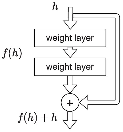
Figure 1. ResNet block.

Moreover, considering a network with D layers, stacking the blocks and representing the discrete transitions at step t in an iterative process, then we have the relation given in (2)

$${\mathbf{H}}^{t+1}={\mathbf{H}}^t+\mathbf{F}({\mathbf{H}}^t,\Theta ),$$

(2)

where $t\in \left\{0,\cdots ,T\right\}$ and $H^T\in {\mathbb{R}}^D$, transitions can be seen as an Euler discretization of the continuous transformation [39].

Neural ODE [33] represents continuous transitions of the network, therefore (2) can be expressed as a dynamical transition and define the solution by the following Cauchy problem for an initial state $X_0$:

$$\left\{\begin{array}{c}\dot{\mathbf{H}}\left(t\right)=\mathbf{F}(t,\mathbf{H}\left(t\right),\Theta )\hfill \\ \mathbf{H}\left(0\right)={\mathbf{X}}_0\hfill \end{array}\right.$$

(3)

A discussion for the well-posedness of (3) is presented in [33,38].

2.2. Training Using ODE Solvers

Solution to (3) is performed through training using ODE solvers. The loss L is calculated using the forward propagation and a first ODE solver as (4).

$$L\left(z\left(t_1\right)\right)=L\left(z\left(t_0\right)+{\int }_{t_0}^{t_1}\mathbf{F}(z\left(t_0\right),t_0,t_1,\Theta )dt\right)=L\left(ODESolve(z\left(t_0\right),\mathbf{F},t_0,t_1,\Theta )\right),$$

(4)

where $z\left(t\right)$ is the hidden state at each instant, $t_0$ and $t_1$ are the initial and final time respectively.

For the backward propagation, Chen et al. [33] proposes the use of adjoint state, $a\left(t\right)=\partial L/\partial z\left(t\right)$, for the calculation of the propagation gradients. The adjoint sensitivity method is applied and the adjoint dynamics are calculated using a backward solver for the relation given in (5)

$$\frac{\partial a\left(t\right)}{\partial t}=-a{\left(t\right)}^{\top }\frac{\partial \mathbf{F}\left(z\right(t),t,\Theta )}{\partial t}.$$

(5)

Computation of the gradient change with respect to the parameters requires to solve relation (6) also backward

$$\frac{\partial L}{\partial \Theta }=-{\int }_{t_1}^{t_0}a{\left(t\right)}^{\top }\frac{\partial \mathbf{F}\left(z\right(t),t,\Theta )}{\partial t}.$$

(6)

Finally, Equations (4)–(6) are implemented as an augmented dynamics that permit to evaluate the respective integrals for z, a and $\frac{\partial L}{\partial \Theta }$ jointly in a single call to the ODE solver. More elaborated details can be found in the original article [33].

2.3. External Inputs

In a system process, some external inputs had to be considered in the system. They are added as dynamical variable into the derivatives, thus modifying (3)

$$\left\{\begin{array}{c}\dot{\mathbf{H}}\left(t\right)=\mathbf{F}(t,\mathbf{H}\left(t\right),\Theta )+u\left(t\right)\hfill \\ \mathbf{H}\left(0\right)={\mathbf{X}}_e\hfill \end{array}\right.$$

(7)

Note that this does not modify the ODE implementation but an additional term has to be included for relation (4), therefore for the integral calculation, the total loss in the system is calculated using (8).

$$L\left(z\left(t_1\right)\right)=L\left(z\left(t_0\right)+{\int }_{t_0}^{t_1}\mathbf{F}(z\left(t_0\right),\mathbf{F},t_0,t_1,\Theta )dt+{\int }_{t_0}^{t_1}u\left(t\right)dt\right).$$

(8)

Meanwhile, Equations (5) and (6) remain the same. Hence, in the ODE layer implementation, as employed in Section 4, Equations (5)–(8) are used.

3. Model Representation

The system representation used is a state-space for nonlinear systems; such representation is employed to have a defined number of system variables that will coincide with the neural ODE outputs; moreover, we describe the signals used in the training of the neural ODE.

3.1. State-Space

We consider a nonlinear state-space representation in the following form:

$$\dot{x}\left(t\right)=f\left(x\right)+g\left(u\right),$$

(9)

$$y\left(t\right)=h\left(x\right),$$

(10)

where $x\left(t\right)\in {\mathbb{R}}^n$ is the state vector, $f(.)$ is a function ${\mathbb{R}}^n\to {\mathbb{R}}^n$, $u\left(t\right)\in {\mathbb{R}}^m$ the input vector, $g(.)$ is a function ${\mathbb{R}}^m\to {\mathbb{R}}^n$, $y\left(t\right)\in {\mathbb{R}}^p$ the output vector, and $h(.)$ is a function ${\mathbb{R}}^n\to {\mathbb{R}}^p$.

Relation (9) is termed the process equation and relation (10) is termed the measurement equation.

3.2. Neural ODE Networks

It is clear that any state-space system in the form given by (9) is composed of a set of ODE systems, here each state $x_i$, where $i=\left\{1,2,\cdots ,n\right\}\in \mathbb{N}$, can be modeled as an output of the neural ODE. Training is challenging since states are not always available, one reasonable solution is to generate an embedding using the measurement equation given by (10), this is the part of the model that we include in the network.

The neural ODE thus has n outputs for which loss calculation is done using the measurements fed through $h\left(x\right)$. Meanwhile, the inputs $u\left(t\right)$ are incorporated as dynamic external inputs in the network. Also, note that knowledge of function $f\left(x\right)$ is not required for the training, since weights and transition functions are learned by the neural ODE. The network can be then especially sensible to faults in the process functions and in the measurement functions as will be proved in the following sections.

4. Fault Diagnosis via Neural ODE Applied to Nonlinear Benchmark System

The fault diagnosis system for a non-linear plant based on the 4-tank model is presented. Hence, the model is first presented, and thereafter the generation and processing of the data-sets are described; since this is a solution for actuators, sensors, and process faults, training and results for each case are presented separately. The schemes used for the neural ODE training and the fault diagnosis training are also presented.

4.1. System Model

A non-linear four-tank plant (Figure 2) is a MIMO benchmark model to evaluate FDI algorithms, first proposed in [40], studied for control [41] and fault diagnosis systems [42]. The system has 2 pumps which are controlled to input water flow into the system, the valve formation distributes the flow into the tanks in a proportion given by the constants ${\gamma }_i$ and $k_i$. The states of the plant are the levels in each tank ($h_i$) and they are related by the following relations:

$$\begin{array}{cc}\hfill {\dot{h}}_1\left(t\right)& =\frac{-a_1\sqrt{2g{h}_1\left(t\right)}}{A_1}+\frac{a_4\sqrt{2g{h}_4\left(t\right)}}{A_1}+\frac{{\gamma }_1{k}_1{u}_1}{A_1\left(t\right)},\hfill \\ \hfill {\dot{h}}_2\left(t\right)& =\frac{-a_2\sqrt{2g{h}_2\left(t\right)}}{A_2}+\frac{a_3\sqrt{2g{h}_3\left(t\right)}}{A_2}+\frac{{\gamma }_2{k}_2{u}_2\left(t\right)}{A_2},\hfill \\ \hfill {\dot{h}}_3\left(t\right)& =\frac{-a_3\sqrt{2g{h}_3\left(t\right)}}{A_3}+\frac{(1-{\gamma }_1)k_1{u}_1\left(t\right)}{A_3},\hfill \\ \hfill {\dot{h}}_4\left(t\right)& =\frac{-a_4\sqrt{2g{h}_4\left(t\right)}}{A_4}+\frac{(1-{\gamma }_2)k_2{u}_2\left(t\right)}{A_4},\hfill \end{array}$$

where the coefficients $A_i$, $a_i$, ${\gamma }_i$ and $k_i$ are described in Table 1. Only parameters related to the inputs are used for the training.

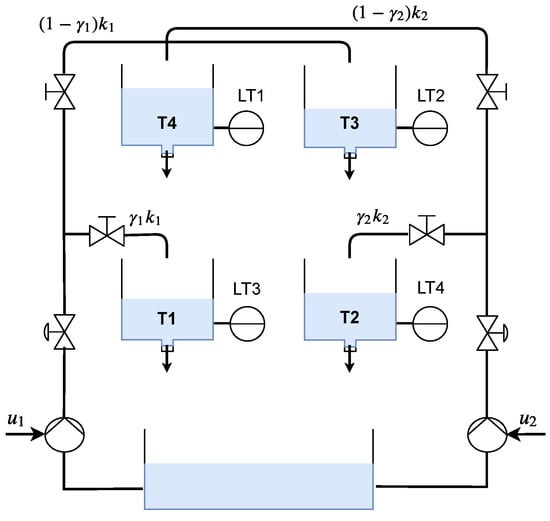
Figure 2. Four tank plant scheme.

Table 1. Process Parameters.

Parameter	Units
Bottom area, $A_i$, for $i=1,2,3,4$	${\mathrm{cm}}^2$
Outlet pipe cross section, $a_i$, for $i=1,2$	$\mathrm{cm}$
Outlet pipe cross section, $a_i$, for $i=3,4$	$\mathrm{cm}$
Gravity constant, g	${\mathrm{cm}}^2/\mathrm{s}$
Pump constants, $k_i$, for $i=1,2$	${\mathrm{cm}}^3/\left(\mathrm{V}\mathrm{s}\right)$
Main valve positions, ${\gamma }_i$ for $i=1,2$
Heights 1 and 2, $h_{1o}$, $h_{2o}$	$\mathrm{cm}$
Heights 3 and 4, $h_{3o}$, $h_{4o}$	$\mathrm{cm}$
Inputs 1 and 2, $u_{1o}$, $u_{2o}$	${\mathrm{cm}}^3/\mathrm{s}$

Hence, for this system, the measurements and state vectors in (11) are considered.

$$y\left(t\right)=\left[\begin{array}{c}{h}_1\left(t\right)\\ h_2\left(t\right)\\ h_3\left(t\right)\\ h_4\left(t\right)\end{array}\right]+\nu \left(t\right),x\left(t\right)=\left[\begin{array}{c}{h}_1\left(t\right)\\ h_2\left(t\right)\\ h_3\left(t\right)\\ h_4\left(t\right)\end{array}\right].$$

(11)

The faults considered are two actuators faults, four sensor faults, and four process faults, we will treat them separately for the training but a complete system can be easily composed by joining the neural models.

4.2. Data-Set

The data-set for the Four Tank Process are generated using the exact model of the system, including typical dynamic possibilities present in the real system, such as controllers, set-point modifications, measurement noise, perturbations, and also actuators, sensors and process faults. A total of 1,000,000 samples are obtained for each case (actuator, sensor, and process fault scenarios), considering only the known signals (measurements and inputs) and the labels for each fault. An extract of the whole data-set is shown in Figure 3, and its corresponding actuator faults are shown in Figure 4.

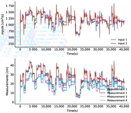
Figure 3. An extract from the data-set of the four tank system. Above: Inputs, Below: Measurements.

Figure 4. Actuator faults in an extract of the data-set, shaded areas indicate that a fault has occurred, and signals are normalized.

4.3. Actuator Faults

4.3.1. Training

Training is performed in two stages, in the first stage the Neural ODE [33] is trained using the block representation presented in Figure 5, the measurements ($y\left(t\right)$) pass through 4 linear layers, where the first three layers are followed by activation functions of Tanh type, meanwhile, the inputs ($u\left(t\right)$) are considered using a linear layer. For this stage, the training is done in 2000 epochs, with a learning rate that starts at ${10}^{-3}$ and is varied at epoch 1000 to ${10}^{-4}$. The ODE tolerance is kept at ${10}^{-7}$ during the whole process. Inputs ($u\left(t\right)$) are added sequentially using a linear layer that is kept constant.

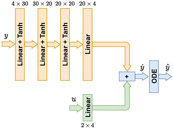
Figure 5. Neural network model for ODE training.

For the second stage of training, one additional linear layer with a Tanh activation function and a softmax classifier for four classes (two actuator faults) are added. The model considered is presented in Figure 6. The input for this stage is the propagated derivatives of the internal states ($\dot{\widehat{y}}$) and the derivatives for the measurements ($\dot{y}$). This training is performed in 20,000 epochs starting with a learning rate of ${10}^{-3}$ that is reduced at epoch 15,000 to ${10}^{-4}$. For simplicity, we kept the model of the first stage, the neural ODE, constant during this second stage training. However, is possible to continue adapting the neural ODE in this stage or even during evaluation for possible model changes.

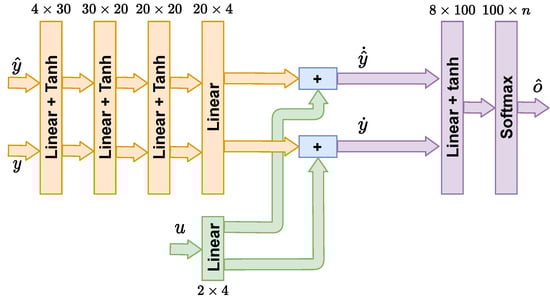
Figure 6. Neural network model for fault diagnosis training.

4.3.2. Results

In order to evaluate the results, we first show in Figure 7 the generated dynamics using the neural network for 2000 points with initial conditions $x=[0,0,0,0]$, that is compared in the same plot with the real system responses, this demonstrates that the network is representing essential information from the model.

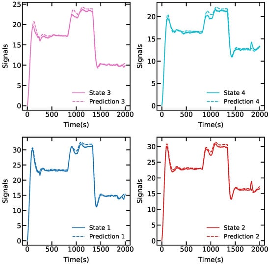
Figure 7. First stage. Continuous line: true dynamics, dotted line: learned dynamics.

For the diagnosis, a total of 20,000 samples from the data-set are used, results are shown in Figure 8, where a comparative of the real faults and detected faults is presented, the network reached 98.73% of accuracy for this test. In the total data-set with 1,000,000 samples, the accuracy was 98.5%.

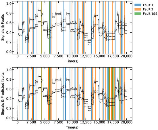
Figure 8. Actuator faults detection, the faults are represented in the shaded areas, states are given in black for reference. Above: faults labeled in the data-set. Below: faults detected by the system.

4.4. Sensor Faults

4.4.1. Training

The first stage of this training is not required since the model is already embedded in the neural ODE from training in Section 4.3.1 using the same scheme presented in Figure 7. For the second stage of training, the model considered is the same as presented in Figure 6 but using a softmax classifier with 16 classes (4 sensor faults). This training is performed in 10,000 epochs starting with a learning rate ${10}^{-3}$ that is reduced at epoch 8000 to ${10}^{-4}$, for simplicity we also kept the model of the first stage constant during this training.

4.4.2. Results

The results for a group of 20,000 samples of the data-set are shown in Figure 9, where a comparative of the real faults and detected faults are given. In this case, the network reached 98.36% of accuracy for this test. On the total data-set, with 1,000,000 samples, the accuracy was 98.1%.

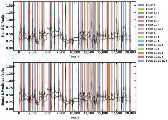
Figure 9. Sensor faults detection, the faults are represented in the shaded areas, states are given in black for reference. Above: faults labeled in the data-set. Below: faults detected by the system.

4.5. Process Faults

4.5.1. Training

In this case, the first stage of training was also not required. For the second stage of training, the model considered was is based as well in the scheme of Figure 6, and the softmax classifier used 16 classes (4 process faults). This training was performed in 30,000 epochs starting with a learning rate ${10}^{-3}$ that is reduced at epoch 20,000 to ${10}^{-4}$, the model of the first stage is kept constant during this training.

4.5.2. Results

The results for a group of 20,000 samples of the data-set are shown in Figure 10, where a comparative of the real faults and detected faults are given. In this case, the network reached 98.75% of accuracy for the test. On the total data-set, with 1,000,000 samples, the accuracy was 98.11%.

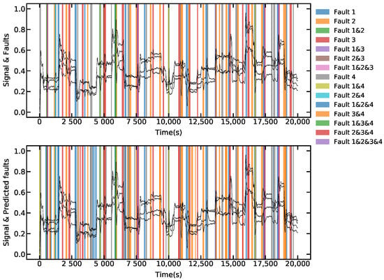
Figure 10. Process faults detection, the faults are represented in the shaded areas, states are given in black for reference. Above: faults labeled in the data-set. Below: faults detected by the system.

5. Visual Representation of the Network

A common pitfall of using DL networks is the lack of visual representation of the neural network which is often seen as a black box. With the proposed approach we furthermore could establish an additional representation for the network, since dynamics in the network follows closely that of the plant, an interesting representation is the phase diagrams generated by the Neural ODE. To illustrate this concept, we present the phase diagram for normal states of the system in Figure 11 and Figure 12 against faulty conditions for actuators and sensors in Figure 13 and Figure 14 respectively. These diagrams are generated using the ODE projection for 200 samples. It is noticeable that continuous predictions are obtained when normal conditions are happening. On the other hand, the predictions are not continuous in the case of faults.

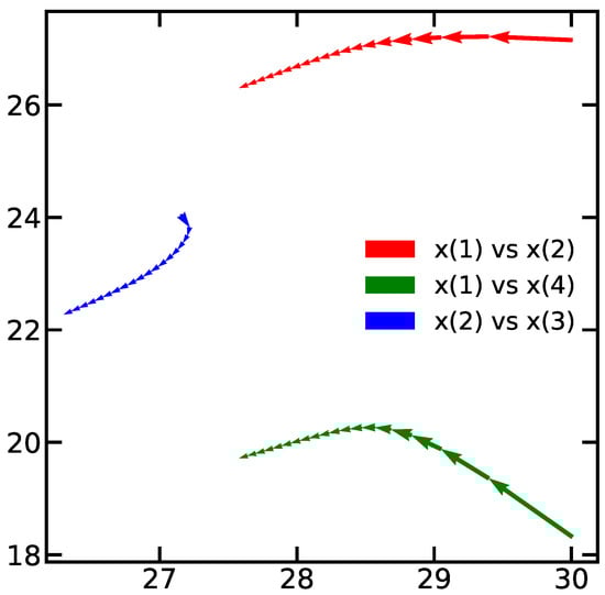
Figure 11. Phase diagram for normal prediction in actuators data-set.

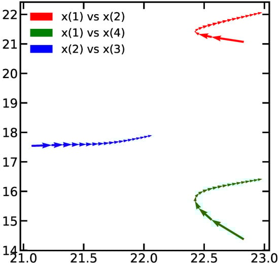
Figure 12. Phase diagram for normal prediction in sensors data-set.

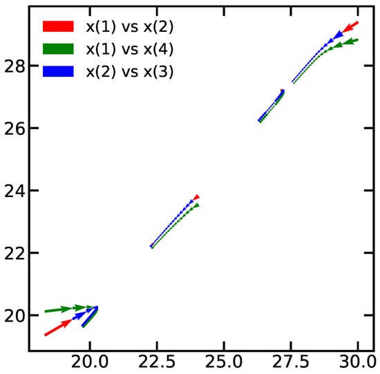
Figure 13. Phase diagram during fault in actuator.

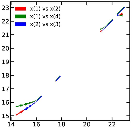
Figure 14. Phase diagram during a fault in sensor.

6. Discussion

Training methodology of DL structures is vital to reach models with high performance. A review of the literature demonstrates that training can be very demanding for DL models. In [43], a common procedure for fault detection using DL models is proposed, feature extraction and neural network type are regarded as two key elements of the process. In [44] an autoencoder is used with 4 different and selectable behaviors. In [21], the training is divided into many steps in accordance with the aging of the system. In [20], the training is performed using ensemble learning, which uses multiple learners. In [25], a feature extraction and a dimensionality reduction are performed previously over the data-set. In [24], a group of 14 features is extracted and then selected using a criterion before the training. All these approaches shown the complexity that features selection requires.

Our approach aims to alleviate these complicated procedures with the inclusion of some characteristics of the model dynamics to be learned by the Neural ODE. We incorporated in the training an approximation of the system using features in form of the measurement equations and inputs of the process. Those characteristics allow us to reduce the epochs and complexity and furthermore to work with data-series in a natural manner, as was demonstrated in Section 4.

Some final tests were performed using classical SVM, ANN, and DL models with the data-set of actuator faults, Table 2 shows the results for each model tested, we include weighted accuracy as a measure for accuracy considering weights for each class, class 0 for no fault is weighted 0.08 and other classes are weighted 0.95, 0.96 and 0.99, respectively. Additionally, in all the deep learning methods, except for the Neural ODE method, data augmentation is previously performed using noise injection, dropout, pooling, and time-warping [45]; and batch normalization is included for the fully connected layers. It is noticeable from the results that the Neural ODE model allows improving the efficiency of the network for this case.

Table 2. Accuracy for different Machine learning Models.

Model	Accuracy	Weighted Accuracy
Suport Vector Machine
(Polynomial Kernel)	93.3%	62.657%
Artificial Neural Network
(4 Fully connected Layers)	80.9%	74.8%
Convolutional Neural Network
(2 Convolutional Layers + 1 Fully connected Layer)	77.5%	55.8%
Recurrent Neural Network
(4 LSTM Layers + 1 Fully connected Layer)	80.53%	73.8%
Neural ODE & Dense Network
(Neural ODE + 2 Fully connected Layers)	98.5%	90%

From Table 2, the SVM method reaches a high accuracy for this case, but it is clearly due to false negatives, as is appreciated in its corresponding weighted accuracy. The ANN and DL models had a lower accuracy; hence, it is likely required a more advanced pre-processing of the data-set to reach better results. Meanwhile, the use of neural ODE and dense network, proposed in this work, shows that, even excluding pre-processing and data augmentation, the model can achieve higher accuracies.

7. Conclusions

Over the past few years, the development of new techniques for deeper networks such as ResNet has inspired the training of neural networks using ODE solvers as a manner to generate a continuous layer representation and even further allowed to improve the representation of systems dynamics by neural ODE networks. Therefore, a hybrid approach was presented in this article for fault diagnosis of sensors, actuators, and process faults. Results of simulations show that high performances of fault diagnosis can be obtained using neural ODE networks not requiring extensive data-processing and advanced modeling. In a nonlinear benchmark system, the training efficiency was demonstrated for each fault type, and shows an improvement when compared with classical Deep Learning models. Here, the accuracy of the network is demonstrated to be higher than 90%. In addition, a visual representation is proposed by using phase diagram representations. Likewise, the data needed to train effectively the network is reduced which permits to avoid elaborated procedures such as feature extraction, pre-processing and data augmentation.

References

- Ding, S.X. Model-Based Fault Diagnosis Techniques, 2nd ed.; Springer: London, UK, 2013. [Google Scholar]
- Pérez-Zuñiga, G.; Rivas-Perez, R.; Sotomayor-Moriano, J.; Sánchez-Zurita, V. Fault Detection and Isolation System Based on Structural Analysis of an Industrial Seawater Reverse Osmosis Desalination Plant. Processes 2020, 8, 1100. [Google Scholar] [CrossRef]
- Krysander, M.; Åslund, J.; Nyberg, M. An efficient algorithm for finding minimal overconstrained subsystems for model-based diagnosis. IEEE Trans. Syst. Man Cybern. Part A Syst. Hum. 2008, 38, 197–206. [Google Scholar] [CrossRef]
- Pérez, C.G.; Travé-Massuyès, L.; Chanthery, E.; Sotomayor, J. Decentralized diagnosis in a spacecraft attitude determination and control system. J. Phys. Conf. Ser. 2015, 659, 1–12. [Google Scholar] [CrossRef]
- Dai, X.; Gao, Z.; Breikin, T.; Wang, H. Disturbance attenuation in fault detection of gas turbine engines: A discrete robust observer design. IEEE Trans. Syst. Man Cybern. Part C Appl. Rev. 2009, 39, 234–239. [Google Scholar] [CrossRef]
- Gao, Z.; Cecati, C.; Ding, S.X. A survey of fault diagnosis and fault-tolerant techniques-part II: Fault diagnosis with knowledge-based and hybrid/active approaches. IEEE Trans. Ind. Electron. 2015, 62, 3768–3774. [Google Scholar] [CrossRef]
- Karimi, H.R.; Zapateiro, M.; Luo, N. A linear matrix inequality approach to robust fault detection filter design of linear systems with mixed time-varying delays and nonlinear perturbations. J. Frankl. Inst. 2010, 347, 957–973. [Google Scholar] [CrossRef]
- Liu, C.; Jiang, B.; Zhang, K. Sliding mode observer-based actuator fault detection for a class of linear uncertain systems. In Proceedings of the 2014 IEEE Chinese Guidance, Navigation and Control Conference, CGNCC 2014, Yantai, China, 8–10 August 2014; pp. 230–234. [Google Scholar] [CrossRef]
- Guo, F.; Ren, X.; Li, Z.; Han, C. Kalman filter based fault detection of dual motor systems. In Proceedings of the Chinese Control Conference, CCC 2017, Dalian, China, 26–28 July 2017; pp. 7133–7137. [Google Scholar] [CrossRef]
- Nguang, S.K.; Zhang, P.; Ding, S. Parity relation based fault estimation for nonlinear systems: An LMI approach. IFAC Proc. Vol. (IFAC-PapersOnline) 2006, 6, 366–371. [Google Scholar] [CrossRef]
- Basri, H.M.; Lias, K.; Abidin, W.A.W.Z.; Tay, K.M.; Zen, H. Fault Detection Using Dynamic Parity Space Approach H. In Proceedings of the 2012 IEEE International PEOCO2012, Melaka, Malaysia, 6–7 June 2012. [Google Scholar]
- Pérez, C.G.; Chanthery, E.; Travé-massuyès, L.; Sotomayor, J. Fault-Driven Minimal Structurally Overdetermined Set in a Distributed Context To cite this version: HAL Id: Hal-01392572, In Proceedings of the 27th International Workshop on Principles of Diagnosis: DX-2016, Denver, CO, USA, 4–7 October 2016.
- Pérez-Zuniga, C.; Chantery, E.; Travé-Massuyes, L.; Sotomayor, J.; Artigues, C. Decentralized Diagnosis via Structural Analysis and Integer Programming. IFAC-PapersOnLine 2018, 51, 168–175. [Google Scholar] [CrossRef]
- Garcia-Alvarez, D. Fault detection using Principal Component Analysis (PCA) in a Wastewater Treatment Plant (WWTP). In Proceedings of the 62-th International Student’s Scientific Conference, San Diego, CA, USA, 17–19 November 2009; p. 6. [Google Scholar]
- Wang, X.; Kruger, U.; Irwin, G.W.; McCullough, G.; McDowell, N. Nonlinear PCA with the local approach for diesel engine fault detection and diagnosis. IEEE Trans. Control Syst. Technol. 2008, 16, 122–129. [Google Scholar] [CrossRef]
- Wang, X.; Liu, X.; Japkowicz, N.; Matwin, S. Ensemble of multiple kernel SVM classifiers. In Lecture Notes in Computer Science (Including Subseries Lecture Notes in Artificial Intelligence and Lecture Notes in Bioinformatics); Springer International Publishing: Cham, Switzerland, 2014; Volume 8436, pp. 239–250. [Google Scholar] [CrossRef]
- Mohd Amiruddin, A.A.A.; Zabiri, H.; Taqvi, S.A.A.; Tufa, L.D. Neural network applications in fault diagnosis and detection: An overview of implementations in engineering-related systems. Neural Comput. Appl. 2020, 32, 447–472. [Google Scholar] [CrossRef]
- Hoang, D.T.; Kang, H.J. A survey on Deep Learning based bearing fault diagnosis. Neurocomputing 2019, 335, 327–335. [Google Scholar] [CrossRef]
- Mandal, S.; Santhi, B.; Sridhar, S.; Vinolia, K.; Swaminathan, P. Nuclear Power Plant Thermocouple Sensor-Fault Detection and Classification Using Deep Learning and Generalized Likelihood Ratio Test. IEEE Trans. Nuclear Sci. 2017, 64, 1526–1534. [Google Scholar] [CrossRef]
- Liang, T.; Wu, S.; Duan, W.; Zhang, R. Bearing fault diagnosis based on improved convolutional deep belief network. IOP Conf. Ser. J. Phys. 2018. [Google Scholar] [CrossRef]
- Jia, F.; Lei, Y.; Lin, J.; Zhou, X.; Lu, N. Deep neural networks: A promising tool for fault characteristic mining and intelligent diagnosis of rotating machinery with massive data. Mech. Syst. Signal Process. 2016, 72–73, 303–315. [Google Scholar] [CrossRef]
- Wei, Z.; Gaoliang, P.; Chuanhao, L. Bearings Fault Diagnosis Based on Convolutional Neural Networks with 2- D Representation of Vibration Signals as Input. MATEC Web Conf. 2017, 13001, 1–5. [Google Scholar]
- Zhang, B.; Li, W.; Hao, J.; Li, X.L.; Zhang, M. Adversarial adaptive 1-D convolutional neural networks for bearing fault diagnosis under varying working condition. arXiv 2018, arXiv:1805.00778. [Google Scholar]
- Guo, L.; Li, N.; Jia, F.; Lei, Y.; Lin, J. A recurrent neural network based health indicator for remaining useful life prediction of bearings. Neurocomputing 2017, 240, 98–109. [Google Scholar] [CrossRef]
- Abed, W.; Sharma, S.; Sutton, R.; Motwani, A. A Robust Bearing Fault Detection and Diagnosis Technique for Brushless DC Motors Under Non-stationary Operating Conditions. J. Control Autom. Electr. Syst. 2015, 26, 241–254. [Google Scholar] [CrossRef]
- Zhang, C.; Xu, L.; Li, X.; Wang, H. A Method of Fault Diagnosis for Rotary Equipment Based on Deep Learning. In Proceedings of the 2018 Prognostics and System Health Management Conference, PHM-Chongqing 2018, Chongqing, China, 26–28 October 2018; pp. 958–962. [Google Scholar] [CrossRef]
- Frank, S.; Heaney, M.; Jin, X.; Robertson, J.; Cheung, H.; Elmore, R.; Henze, G.P. Hybrid Model-Based and Data-Driven Fault Detection and Diagnostics for Commercial Buildings. In Proceedings of the ACEEE Summer Study on Energy Efficiency in Buildings, Pacific Grove, CA, USA, 21–26 August 2016; pp. 12.1–12.4. [Google Scholar]
- Jung, D.; Ng, K.Y.; Frisk, E.; Krysander, M. A combined diagnosis system design using model-based and data-driven methods. In Proceedings of the Conference on Control and Fault-Tolerant Systems, SysTol, Barcelona, Spain, 7–9 September 2016; pp. 177–182. [Google Scholar] [CrossRef]
- Jung, D.; Ng, K.Y.; Frisk, E.; Krysander, M. Combining model-based diagnosis and data-driven anomaly classifiers for fault isolation. Control Eng. Pract. 2018, 80, 146–156. [Google Scholar] [CrossRef]
- Jung, D.; Sundstrom, C. A Combined Data-Driven and Model-Based Residual Selection Algorithm for Fault Detection and Isolation. IEEE Trans. Control Syst. Technol. 2019, 27, 616–630. [Google Scholar] [CrossRef]
- Jiang, N.; Hu, X.; Li, N. Graphical temporal semi-supervised deep learning–based principal fault localization in wind turbine systems. Proc. Inst. Mech. Eng. Part I J. Syst. Control Eng. 2020, 234, 985–999. [Google Scholar] [CrossRef]
- Li, D.; Wang, Y.; Wang, J.; Wang, C.; Duan, Y. Recent advances in sensor fault diagnosis: A review. Sens. Actuators A Phys. 2020, 309, 111990. [Google Scholar] [CrossRef]
- Chen, R.T.Q.; Rubanova, Y.; Bettencourt, J.; Duvenaud, D. Neural Ordinary Differential Equations. arXiv 2018, arXiv:1806.07366. [Google Scholar]
- He, K.; Zhang, X.; Ren, S.; Sun, J. Deep residual learning for image recognition. In Proceedings of the IEEE Computer Society Conference on Computer Vision and Pattern Recognition, Las Vegas, NV, USA, 27–30 June 2016; pp. 770–778. [Google Scholar] [CrossRef]
- Deng, Z.; Nawhal, M.; Meng, L.; Mori, G. Continuous Graph Flow. arXiv 2019, arXiv:908.02436. [Google Scholar]
- Greydanus, S.; Dzamba, M.; Yosinski, J. Hamiltonian Neural Networks. arXiv 2019, arXiv:1906.01563v3. [Google Scholar]
- Tzen, B.; Raginsky, M. Neural Stochastic Differential Equations: Deep Latent Gaussian Models in the Diffusion Limit. arXiv 2019, arXiv:1905.09883v2. [Google Scholar]
- Poli, M.; Massaroli, S.; Park, J.; Yamashita, A.; Asama, H.; Park, J. Neural ordinary differential equations. In Proceedings of the Advances in Neural Information Processing Systems, Virtual, 6–12 December 2020; pp. 6571–6583. [Google Scholar]
- Ruthotto, L.; Haber, E. Deep Neural Networks Motivated by Partial Differential Equations. J. Math. Imaging Vis. 2020, 62, 352–364. [Google Scholar] [CrossRef]
- Johansson, K.H. The quadruple-tank process: A multivariable laboratory process with an adjustable zero. IEEE Trans. Control Syst. Technol. 2000, 8, 456–465. [Google Scholar] [CrossRef]
- Sotomayor-Moriano, J.; Pérez-Zúñiga, G.; Soto, M. A Virtual Laboratory Environment for Control Design of a Multivariable Process. IFAC PapersOnLine 2019, 52, 218–223. [Google Scholar] [CrossRef]
- Sánchez-Zurita, V.; Pérez-Zúñiga, G.; Sotomayor-Moriano, J. Reconfigurable Model Predictive Control applied to the Quadruple Tank Process. In Proceedings of the 15th European Workshop on Advanced Control and Diagnosis, Palazzo Grassi, Bologna, 21–22 November 2019. [Google Scholar]
- Jager, G.; Zug, S.; Brade, T.; Dietrich, A.; Steup, C.; Moewes, C.; Cretu, A.M. Assessing neural networks for sensor fault detection. In Proceedings of the CIVEMSA 2014—2014 IEEE Conference on Computational Intelligence and Virtual Environments for Measurement Systems and Applications, Ottawa, ON, Canada, 5–7 May 2014; pp. 70–75. [Google Scholar] [CrossRef]
- Shao, H.; Jiang, H.; Zhao, H.; Wang, F. A novel deep autoencoder feature learning method for rotating machinery fault diagnosis. Mech. Syst. Signal Process. 2017, 95, 187–204. [Google Scholar] [CrossRef]
- Wen, Q.; Sun, L.; Song, X.; Gao, J.; Wang, X.; Xu, H. Time Series Data Augmentation for Deep Learning: A Survey. arXiv 2020, arXiv:2002.12478. [Google Scholar]
Publisher’s Note: MDPI stays neutral with regard to jurisdictional claims in published maps and institutional affiliations. |
© 2021 by the authors. Licensee MDPI, Basel, Switzerland. This article is an open access article distributed under the terms and conditions of the Creative Commons Attribution (CC BY) license (http://creativecommons.org/licenses/by/4.0/).